![]()
Parallel Data Warehouse Patterns
Microsoft’s SQL Server Parallel Data Warehouse (PDW) appliance was introduced with SQL Server 2008 R2 and is Microsoft’s first massively parallel processing (MPP) offering. Although PDW is built upon the SQL Server platform, it is a completely different product. As the name suggests, MPP uses multiple servers working as one system, called an appliance, to achieve much greater performance and scan rates than in traditional SMP systems. SMP refers to symmetric multi-processing; most database systems, such as all other versions of SQL Server, are SMP.
To obtain a better understanding of the difference between SMP and MPP systems, let’s examine a common analogy. Imagine you are handed a shuffled deck of 52 playing cards and asked to retrieve all of the Queens. Even at your fastest, it would take you several seconds to retrieve the requested cards. Let’s now take that same deck of 52 cards and divide it across ten people. No matter how fast you are, these ten people working together can retrieve all of the Queens much faster than you can by yourself.
As you may have inferred, you represent the SMP system, and the ten people represent the MPP system. This divide-and-conquer strategy is why MPP appliances are particularly well suited for high-volume, scan-intensive data warehousing environments, especially ones that need to scale to hundreds of terabytes of storage. There are other MPP appliance vendors available besides Microsoft; however, close integration with the Microsoft business intelligence stack (SQL Server, Integration Services, Analysis Services, and Reporting Services) and a compelling cost-per-terabyte make PDW a natural progression for organizations needing to take their SQL Server data warehouse to the next level. In this chapter, we will walk through how to load data into the PDW appliance using Integration Services. But first we will need to discuss some of the differences between PDW and SMP SQL Server.
PDW is built upon the SQL Server platform but has an architecture entirely its own. While the details of this architecture could easily consume a book in its own right, we will only cover the most pertinent parts to ensure you have the foundation necessary for loading data.
![]() Tip Learn more about Microsoft’s Parallel Data Warehouse at http://microsoft.com/pdw and http://sqlpdw.com.
Tip Learn more about Microsoft’s Parallel Data Warehouse at http://microsoft.com/pdw and http://sqlpdw.com.
Before we proceed, it is important to note that only SQL Server 2008 R2 Business Intelligence Studio (BIDS) was supported at the time of writing for the creation of Integration Services packages to load data into PDW. Thus, this chapter will depart from the rest of the book in that it uses BIDS for its screenshots. Also, an actual PDW appliance is required to execute the samples in this chapter. For those who do not have a PDW appliance, there is still much information that can be gathered from this chapter regarding PDW architecture and loading best practices.
Each PDW appliance has one control rack and one or more data racks. The control rack contains the following nodes:
- Control Node – Perhaps the most critical node in the appliance, the Control Node is responsible for managing the workload, creating distributed query plans, orchestrating data loads, and monitoring system operations.
- Management Node – Among other administrative functions, the management node is responsible for authentication, software updates, and system monitoring.
- Backup Node – As the name suggests, this is where backups are stored.
- Landing Zone Node – This is the node that is most relevant to this chapter. The Landing Zone node is the only node in the entire appliance that is accessible for loading data.
![]() Tip Microsoft recommends running Integration Services packages from an external server. This best practice reduces memory contention on the Landing Zone. If this type of server is not within your budget, you can purchase and install SQL Server Integration Services on the Landing Zone to facilitate package execution and job scheduling through SQL Agent Jobs.
Tip Microsoft recommends running Integration Services packages from an external server. This best practice reduces memory contention on the Landing Zone. If this type of server is not within your budget, you can purchase and install SQL Server Integration Services on the Landing Zone to facilitate package execution and job scheduling through SQL Agent Jobs.
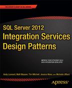
Figure 8-1 depicts a single data-rack PDW configuration. Each PDW appliance is comprised of one or more data racks but only a single control rack. In every data rack are ten Compute Nodes, plus one hot-spare standby Compute Node for high availability.
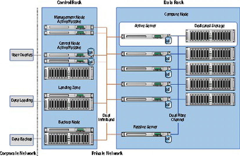
Figure 8-1. A single data-rack PDW configuration
At the core of PDW is the concept of “shared-nothing” architecture, where a single logical table is broken up into numerous smaller pieces. The exact number of pieces depends on the number of data racks you have. Each of these smaller pieces is then stored on a separate Compute Node. Within a single Compute Node, each data piece is then split across 8 distributions. Furthermore, each of these 8 distributions has its own dedicated CPU, memory, and LUNs (hence the term “shared-nothing”). There are numerous benefits that a shared-nothing architecture enables, such as more linear scalability. But perhaps PDW’s greatest power is its ability to scan data at incredible speeds.
Let’s do some math. Assume we have a PDW appliance with one data rack, and we need to store a table with one billion rows. Each Compute Node will store 1/10th of the rows, and each Compute Node will split its data across 8 distributions. Thus, the one billion row table will be split into 80 pieces (10 Compute Nodes x 8 distributions each). That means each distribution will store 12,500,000 rows.
But what does this mean from the end-user’s standpoint? Let’s look at a hypothetical situation. You are a user who needs to submit a query that joins two tables together: a Sales table with one billion rows, and a Customer table with 50 million rows. And, as luck would have it, there are no indexes available that will cover your query. This means you will need to scan, or read, every row in each table.
In an SMP system – where memory, storage, and CPU are shared – this query could take hours or days to run. On some systems, it might not even be feasible to attempt this query, depending on factors such as the server hardware and the amount of activity on the server. Suffice it to say, the query will take a considerable amount of time to return and will most likely have a negative impact on other activity on the server.
In PDW, these kinds of queries often return in minutes – and a well-designed schema can even execute this query in seconds. This is because the hardware is optimized for scans; PDW expects to scan every row in the table. Remember how we said that every distribution has its own dedicated CPU, memory, and storage? Well, when you submit the query to join one billion rows to 50 million rows, each distribution is performing a scan on its own Sales table of 12,500,000 rows and Customer table with 625,000 rows. Not nearly as intimidating, is it? The data is then sent back to the Control Node across an ultra-fast Dual-Infiniband channel to consolidate the results and return the data to the end user. It is this divide-and-conquer strategy that results in PDW significantly outperforming SMP systems.
PDW is also able to load data very efficiently. As previously mentioned, data is brought into the appliance through the Landing Zone. Each Compute Node then uses a hashing algorithm to determine where to store the data – down to the individual distribution and associated LUNs. A relatively small amount of overhead is associated with this process. Because this overhead is incurred on every single load, transactional load patterns (i.e., singleton inserts) should be avoided. PDW performs at its best when data is loaded in large, incremental batches – you will see much better performance loading 10 files with 100,000 rows each than loading 1,000,000 rows individually, but you will see the best performance loading one file with 1,000,000 rows.
Data can be imported from numerous platforms, including from Oracle, SQL Server, MySQL, and flat files. There are two primary methods of loading data into the PDW appliance: DWLoader and Integration Services. We will briefly discuss when to use DWLoader versus Integration Services. After that, we will actually walk through an example of loading data from SQL Server using Integration Services.
DWLoader vs. Integration Services
DWLoader is a command-line utility that ships with PDW. Those familiar with SQL Server BCP (bulk copy program) will have an easy time learning DWLoader, as both utilities share a very similar syntax. One very common pattern for loading data into PDW from SQL Server is to:
- Export data from SQL Server to a flat file using BCP
- Relocate the data file to the Landing Zone
- Import the data file to PDW using DWLoader
This is a very efficient method for loading data, and it is very easy to generate scripts for table DDL, BCP commands, and DWLoader commands. For this reason, you may want to consider DWLoader for performing initial and incremental loading of the large quantity of small dimensional tables that often exist in data warehouses. Doing so can greatly speed up data warehouse migration. This same load pattern can also be used with flat files generated from any system, not just SQL Server.
For your larger tables, you may instead want to consider Integration Services. Integration Services offers greater functionality and arguably more end-to-end convenience. This is because Integration Services is able to connect directly to the data source and load the data into the PDW appliance without having to stop at a file share. Integration Services can also perform transformations in flight, which DWLoader does not support.
It’s important to note that each Data Flow within Integration Services is single-threaded and can bottleneck on IO. Typically, a single-threaded Integration Services package will perform up to ten times slower than DWLoader. However, a multi-threaded Integration Services package – similar to the one we will create shortly – can mitigate that limitation. For large tables requiring data type conversions, an Integration Services package with 10 parallel Data Flows provides the best of both worlds: similar performance to DWLoader and all the advanced functionality that Integration Services offers.
A number of variables should be considered when deciding whether to use DWLoader or Integration Services. In addition to table size, the network speed and table design can have an impact. At the end of the day, most PDW implementations will use a combination of both tools. The best idea is to test the performance of each method in your environment and use the tool that makes the most sense for each table.
Many Integration Services packages are designed using an Extract, Transform, and Load (ETL) process. This is a practical model that strives to lessen the impact of moving data on the source and destination servers – which are traditionally more resource-constrained – by placing the burden of data filtering, cleansing, and other such activities on the (arguably more easy-to-scale) ETL server. Extract, Load, and Transform (ELT) processes, in contrast, place the burden on the destination server.
While both models have their place and while PDW can support both models, ELT clearly performs better with PDW from both a technical and business perspective. On the technical side, PDW is able to utilize its massively parallel processing power to more efficiently load and transform large volumes of data. From the business aspect, having more data co-located allows more meaningful data to be gleaned during the transformation process. Organizations with MPP systems often find that the ability to co-locate and transform large quantities of disparate data allows them to make the leap from reactive data marts (How much of this product did we sell?) to predictive data modeling (How can we sell more of this product?).
Deciding on an ELT strategy does not necessarily mean your Integration Services package will not have to perform any transformations, however. In fact, many Integration Services packages may require transformations of some sort to convert data types. Table 8-1 illustrates the data types supported in PDW and the equivalent Integration Services data types.
Table 8-1. Data Type Mappings for PDW and Integration Services
| SQL Server PDW Data Type | Integration Services Data Type(s) That Map to the SQL Server PDW Data Type | ||||||
|---|---|---|---|---|---|---|---|
| BIT | DT_BOOL | ||||||
| BIGINT | DT_I1, DT_I2, DT_I4, DT_I8, DT_UI1, DT_UI2, DT_UI4 | ||||||
| CHAR | DT_STR | ||||||
| DATE | DT_DBDATE | ||||||
| DATETIME | DT_DATE, DT_DBDATE, DT_DBTIMESTAMP, DT_DBTIMESTAMP2 | ||||||
| DATETIME2 | DT_DATE, DT_DBDATE, DT_DBTIMESTAMP, DT_DBTIMESTAMP2 | ||||||
| DATETIMEOFFSET | DT_WSTR | ||||||
| DECIMAL | DT_DECIMAL, DT_I1, DT_I2, DT_I4, DT_I4, DT_I8, DT_NUMERIC, | ||||||
| DT_UI1, DT_UI2, DT_UI4, DT_UI8 | |||||||
| FLOAT | DT_R4, DT_R8 | ||||||
| INT | DT_I1, DTI2, DT_I4, DT_UI1, DT_UI2 | ||||||
| MONEY | DT_CY | ||||||
| NCHAR | DT_WSTR | ||||||
| NUMERIC | DT_DECIMAL, DT_I1, DT_I2, DT_I4, DT_I8, DT_NUMERIC, | ||||||
| DT_UI1, DT_UI2, DT_UI4, DT_UI8 | |||||||
| NVARCHAR | DT_WSTR, DT_STR | ||||||
| REAL | DT_R4 | ||||||
| SMALLDATETIME | DT_DBTIMESTAMP2 | ||||||
| SMALLINT | DT_I1, DT_I2, DT_UI1 | ||||||
| SMALLMONEY | DT_R4 | ||||||
| TIME | DT_WSTR | ||||||
| TINYINT | DT_I1 | ||||||
| VARBINARY | DT_BYTES | ||||||
| VARCHAR | DT_STR |
Also, it is worth noting that PDW does not currently support the following data types at the time of this writing:
- DT_DBTIMESTAMPOFFSET
- DT_DBTIME2
- DT_GUID
- DT_IMAGE
- DT_NTEXT
- DT_TEXT
Any of these unsupported data types will need to be converted to a compatible data type using the Data Conversion transformation. We will walk through how to perform such a transformation in just a moment.
Installing the PDW Destination Adapter
As we have previously discussed, data is loaded into the PDW through the Landing Zone. All Integration Services packages will either be run from the Landing Zone node or, preferably, from a non-appliance server with access to the Landing Zone. The 32-bit destination adapter is required for Integration Services and should be installed on the server running the packages. If you are using a 64-bit machine, you will need to install both the 32-bit and 64-bit adapters. The Windows Installer packages are accessible from C:PDWINSTmediamsi on both the Management node and the Landing Zone node, or from the network share at \ < Landing Zone IP Address > edistr.
Once the PDW destination adapter has been installed, you will need to add it to the Integration Services Toolbox. Let’s walk through how to do this now. Start a new Integration Services Project and name it PDW_Example. After the project loads, select Tools from the main menu, and then navigate to Choose Toolbox Items, as illustrated in Figure 8-2.
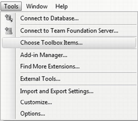
Figure 8-2. Select “Choose Toolbox Items . . .” to add the PDW adapter to Integration Services
Once the Choose Toolbox Items modal appears, click on the SSIS Data Flow Items tab. Navigate down to SQL Server PDW Destination and check the box to the left of the adapter, as illustrated in Figure 8-3. Click OK.
Figure 8-3. The “SSIS Data Flow Items” toolbox
The PDW Destination Adapter is now installed. Let’s move on to setting up our data source.
In preparation for moving data from SQL Server to PDW, we need to create a database in SQL Server and populate it with some test data. Execute the T-SQL code in Listing 8-1 from SQL Server Management Studio (SSMS) to create a new database called PDW_Source_Example.
Listing 8-1. Example of T-SQL Code to Create a SQL Server Database
USE [master];GO
/* Create a database to experiment with */
CREATE DATABASE [PDW_Source_Example]
	ON PRIMARY
	(NAME = N'PDW_Source_Example' ,	FILENAME = N'C:Program FilesMicrosoft SQL ServerMSSQL11.MSSQLSERVERMSSQLDATAPDW_Source_Example.mdf'
 ,	SIZE = 1024MB
 ,	MAXSIZE = UNLIMITED
 ,	FILEGROWTH = 1024MB
	)
	LOG ON
	(
 NAME = N'PDW_Source_Example_log'
 ,	FILENAME = N'C:Program FilesMicrosoft SQL ServerMSSQL11.MSSQLSERVERMSSQLDATAPDW_Source_Example_log.ldf'
 ,	SIZE = 256MB
 ,	MAXSIZE = UNLIMITED
 ,	FILEGROWTH = 256MB
	);
GO
Please note that your database file path may vary depending on the details of your particular installation.
Now let’s create a table and populate it with some data. As we discussed before, Integration Services works best with large tables that can be multi-threaded. One good example of this is a Sales Fact table that is partitioned by year. Listing 8-2 will provide the T-SQL code to create the table and partitioning dependencies.
Listing 8-2. Example of T-SQL Code to Create a Partitioned Table in SQL Server
USE PDW_Source_Example;
GO

/* Create your partition function */
CREATE PARTITION FUNCTION example_yearlyDateRange_pf
(DATETIME) AS RANGE RIGHT
FOR VALUES('2010-01-01', '2011-01-01', '2012-01-01'),
GO

/* Associate your partition function with a partition scheme */
CREATE PARTITION SCHEME example_yearlyDateRange_psAS PARTITION
example_yearlyDateRange_pf ALL TO([Primary]);
GO

/* Create a partitioned fact table to experiment with */
CREATE TABLE PDW_Source_Example.dbo.FactSales (
   orderID      INT IDENTITY(1,1)
   , orderDate  DATETIME
   , customerID INT
   , webID      UNIQUEIDENTIFIER DEFAULT (NEWID())
   CONSTRAINT PK_FactSales
      PRIMARY KEY CLUSTERED
     (
           orderDate
          , orderID
     )
) ON example_yearlyDateRange_ps(orderDate);
![]() Note Getting an error on the above syntax? Partitioning is a feature only available in SQL Server Enterprise and Developer editions. You can comment out the partitioning in the last line:
Note Getting an error on the above syntax? Partitioning is a feature only available in SQL Server Enterprise and Developer editions. You can comment out the partitioning in the last line:
Next, we need to generate data using the T-SQL in Listing 8-3. This is the data we will be loading into PDW.
Listing 8-3. Example of T-SQL Code to Populate a Table with Sample Data
/* Declare variables and initialize with an arbitrary date */
DECLARE @startDate DATETIME = '2010-01-01';

/* Perform an iterative insert into the FactSales table */
WHILE @startDate < GETDATE()
BEGIN

      INSERT INTO PDW_Source_Example.dbo.FactSales
      (orderDate, customerID)
      SELECT @startDate
            , DATEPART(WEEK, @startDate) + DATEPART(HOUR, @startDate);
      /* Increment the date value by hour; for more test data,
      replace HOUR with MINUTE or SECOND */
      SET @startDate = DATEADD(HOUR, 1, @startDate);
END;
This script will generate roughly twenty thousand rows in the FactSales table, although you can easily increase the number of rows generated by replacing HOUR in the DATEADD statement with MINUTE or even SECOND.
Now that we have a data source to work with, we are ready to start working on our Integration Services package.
The Data Flow
We are now going to configure the Data Flow that will move data from SQL Server to PDW. We will first create a connection to our data source via an OLE DB Source. We will transform the UNIQUEIDENTIFIER to a Unicode string (DT_WSTR) using a Data Conversion. We will then configure our PDW Destination Adapter to load data into the PDW appliance. Lastly, we will multi-thread the package to improve load performance.
One easy way to multi-thread is to create multiple Data Flows that execute in parallel for the same table. You can have up to 10 simultaneous loads – 10 Data Flows – for a table. However, you want to be careful not to cause too much contention. You can limit contention by querying on the clustered index or, if you have SQL Server Enterprise Edition, separating the loads by partition. This latter method is preferable and is the approach our example will use.
If you have not already done so, create a new Integration Services Project named PDW_Example (File ![]() New
New ![]() Project
Project ![]() Integration Services Project).
Integration Services Project).
Add a Data Flow Task to the Control Flow designer surface. Name it PDW Import.
Add an OLE DB Source to the designer surface from the SSIS Toolbox. Edit the properties of the OLE DB Source by double-clicking on the icon. You should see the source editor shown in Figure 8-4.
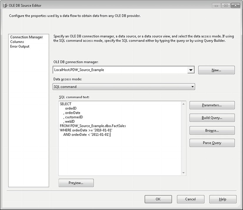
Figure 8-4. The OLE DB Source Editor
You will need to create an OLE DB Connection Manager that points to the PDW_Source_Example database. Once this is done, change the Data Access Mode to SQL Command, then enter the code in Listing 8-4. You should see results similar to those in Figure 8-4. Click OK when finished entering the code.
Listing 8-4. Example SQL Command
/* Retrieve sales for 2010 */
     SELECT
     orderID
     , orderDate
     , customerID
     , webID
     FROM PDW_Source_Example.dbo.FactSales
     WHERE orderDate = = '2010-01-01'
          AND orderDate < '2011-01-01';
Let’s take a minute to discuss what we’re doing. By searching our FactSales table on orderDate – the column we specified as our partitioning key in Listing 8-2 – we are able to achieve partition elimination. This gives us a clean way to divide the multiple Data Flows while also minimizing resource contention. We can achieve a similar result even without partitioning FactSales, because we would still be performing the search on our clustered index. But what if FactSales was clustered on just orderID instead? We can apply the same principles and achieve good performance by searching for an evenly distributed number of rows in each Data Flow. For example, if FactSales has one million rows and we are using 10 Data Flows, each OLE DB Source should search for 100,000 rows (i.e. orderID > = 1 and orderID < 100000; orderID > = 100000 and orderID < 200000; and so on). These types of design considerations can have a significant impact on the overall performance of your Integration Services package.
![]() Tip Not familiar with partitioning? Table partitioning is particularly well suited for large data warehouse environments and offers more than just the benefits briefly mentioned here. More information is available in the whitepaper, “Partitioned Table and Index Strategies Using SQL Server 2008,” at http://msdn.microsoft.com/en-us/library/dd578580.aspx.
Tip Not familiar with partitioning? Table partitioning is particularly well suited for large data warehouse environments and offers more than just the benefits briefly mentioned here. More information is available in the whitepaper, “Partitioned Table and Index Strategies Using SQL Server 2008,” at http://msdn.microsoft.com/en-us/library/dd578580.aspx.
Remember how PDW does not currently support DT_GUID? Our source table has a UNIQUEIDENTIFIER column that is stored as a CHAR(38) column in PDW. In order to load this data, we will need to transform our UNIQUEIDENTIFER to a Unicode string. To do this, drag the Data Conversion icon from the SSIS Toolbox to the designer surface. Next, connect the green line from OLE DB Source to Data Conversion, as shown in Figure 8-5.
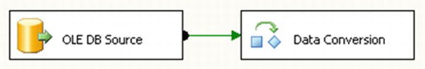
Figure 8-5. Connecting the OLE DB Source to the Data Conversion
Double-click on the Data Conversion icon to open the Data Conversion Transformation Editor. Click on the box to the left of webID, then edit its properties to reflect the following values:
- Input Column: webID
- Output Alias: converted_webID
- Data Type: string [DT_WSTR]Length: 38
Confirm that the settings match those in Figure 8-6, then click OK.
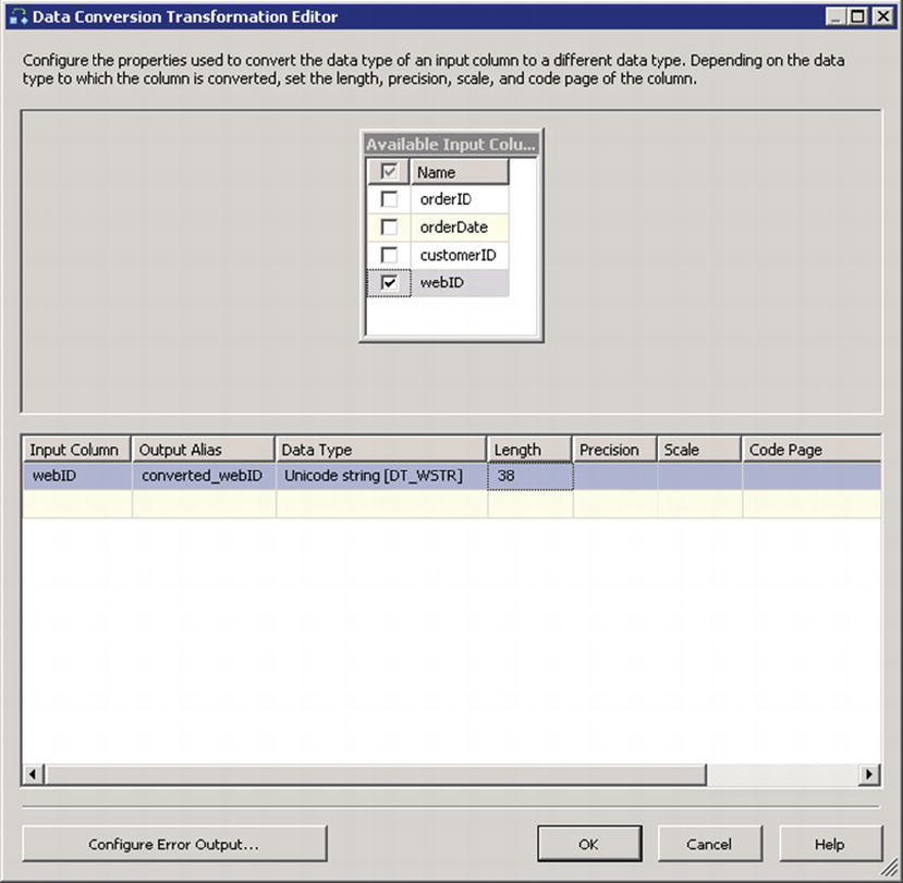
Figure 8-6. The Data Conversion Transformation Editor
![]() Tip Wonder why we use a string length of 38 when converting a UNIQUEIDENTIFIER to a CHAR? This is because the global representation of a GUID is {00000000-0000-0000-0000-000000000000}. The curly brackets are stored implicitly in SQL Server for UNIQUEIDENTIFIER columns. Thus, during conversion, Integration Services materializes the curly brackets for export to the destination system. That is why, while a UNIQUEIDENTIFIER may look like it would only consume 36 bytes, it actually requires 38 bytes to store in PDW.
Tip Wonder why we use a string length of 38 when converting a UNIQUEIDENTIFIER to a CHAR? This is because the global representation of a GUID is {00000000-0000-0000-0000-000000000000}. The curly brackets are stored implicitly in SQL Server for UNIQUEIDENTIFIER columns. Thus, during conversion, Integration Services materializes the curly brackets for export to the destination system. That is why, while a UNIQUEIDENTIFIER may look like it would only consume 36 bytes, it actually requires 38 bytes to store in PDW.
The next few tasks, which prepare the PDW appliance for receiving FactSales data, will take place in the Nexus Query Chameleon – or just Nexus, for short. Nexus, illustrated in Figure 8-7, is a 3rd party tool used for connecting to the PDW appliance. This is currently the recommended graphical query editor for working with PDW, although SQL Server Management Studio (SSMS) will support PDW in future releases.
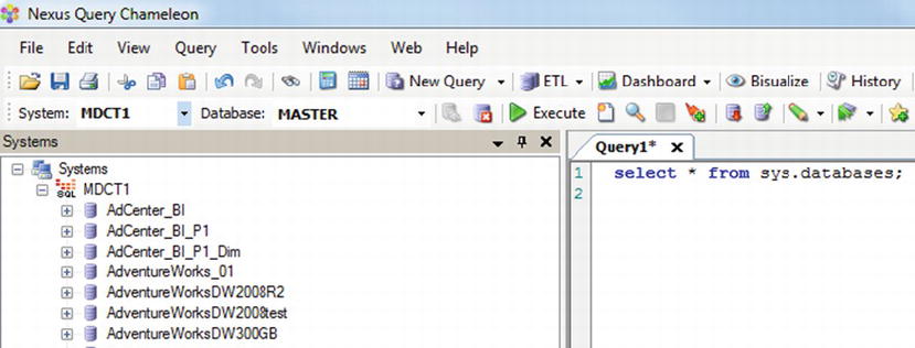
Figure 8-7. The Nexus Query Tool
Please refer to the section “Connect With Nexus Query Chameleon” in the PDW Books Online for more information on installing and configuring Nexus.
Before we go any further, we should discuss the use of a staging database. While it is not required, Microsoft recommends the use of a staging database during incremental loads to reduce table fragmentation. When a staging database is used, the data is first loaded into a temporary table in the staging database before insertion into the permanent table in the destination database.
![]() Tip Using a staging database? Make sure your staging database has enough space available to accommodate all tables being loaded concurrently. If you do not allocate enough space initially, don’t worry; you’ll still be okay – the staging database will autogrow. Your loads may just slow down while the autogrow is occurring. Also, your staging database will likely need to be larger when you perform the initial table loads during system deployment and migration. However, once your system becomes more mature and the initial ramp-up is complete, you can recover some space by dropping and recreating a smaller staging database.
Tip Using a staging database? Make sure your staging database has enough space available to accommodate all tables being loaded concurrently. If you do not allocate enough space initially, don’t worry; you’ll still be okay – the staging database will autogrow. Your loads may just slow down while the autogrow is occurring. Also, your staging database will likely need to be larger when you perform the initial table loads during system deployment and migration. However, once your system becomes more mature and the initial ramp-up is complete, you can recover some space by dropping and recreating a smaller staging database.
From within Nexus, execute the code in Listing 8-5 on your PDW appliance to create a staging database.
Listing 8-5. PDW Code to Run from Nexus to Create a Staging Database
CREATE DATABASE StageDB_Example
WITH
(
                    AUTOGROW           = ON
                , REPLICATED_SIZE    = 1 GB
                , DISTRIBUTED_SIZE = 5 GB
                , LOG_SIZE = 1 GB
);
PDW introduces the concept of replicated and distributed tables. In a distributed table, the data is split across all nodes using a distribution hash specified during table creation. In a replicated table, the full table data exist on every Compute Node. This is done to improve join performance. As a hypothetical example, consider a small DimCountry dimension table with 200 rows. DimCountry would likely be replicated, whereas a much larger FactSales table would be distributed. This design allows any joins between FactSales and DimCountry to take place locally on each node. Although we would essentially be creating ten copies of DimCountry – one on each Compute Node – because the dimension table is small, the benefit of performing the join locally outweighs the minimal cost of storing duplicate copies of the data.
Let’s take another look at our CREATE DATABASE code in Listing 8-5. REPLICATED_SIZE specifies space allocation for replicated tables on each Compute Node, whereas DISTRIBUTED_SIZE specifies space allocation for distributed tables across the appliance. That means StageDB_Example actually has 16 GB of space allocated: 10 GB for replicated tables (10 Compute Nodes with 1 GB each), 5 GB for distributed tables, and 1 GB for the log.
All data is automatically compressed using page-level compression during the PDW load process. This is not optional, and the amount of compression will vary greatly from customer-to-customer and table-to-table. If you have SQL Server Enterprise or Developer Editions, you can execute the command in Listing 8-6 to estimate compression results.
Listing 8-6. Code to Create the Destination Database and Table Inside of PDW
/* Estimate compression ratio */
EXECUTE
sp_estimate_data_compression_savings
'dbo', 'FactSales', NULL, NULL, 'PAGE';
You can generally use 2:1 as a rough estimate. With a 2:1 compression ratio, the 5 GB of distributed data we specified in Listing 8-5 actually stores 10 GB of uncompressed SQL Server data.
We still need a place to store our data. Execute the code in Listing 8-7 in Nexus to create the destination database and table for FactSales.
Listing 8-7. PDW Code to Create the Destination Database and Table
CREATE DATABASE PDW_Destination_Example
WITH
     REPLICATED_SIZE = 1 GB
         , DISTRIBUTED_SIZE = 5 GB
         , LOG_SIZE = 1 GB
);
CREATE TABLE PDW_Destination_Example.dbo.FactSales
(
            orderID
            INT
            , orderDate DATETIME
            , customerID INT
            , webID CHAR(38)
)
WITH
(
            CLUSTERED INDEX (orderDate)
            , DISTRIBUTION = HASH (orderID)
);
Now that we have our destination objects created, we can return to our Integration Services package. From within BIDS, drag the SQL Server PDW Destination from the Toolbox to the Data Flow pane. Double-click on the PDW Destination, illustrated in Figure 8-8, to edit its configuration.
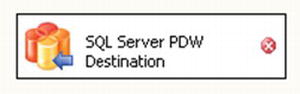
Figure 8-8. The SQL Server PDW Destination
Next, click on the down arrow next to Connection Manager and select Create a New Connection, as shown in Figure 8-9.
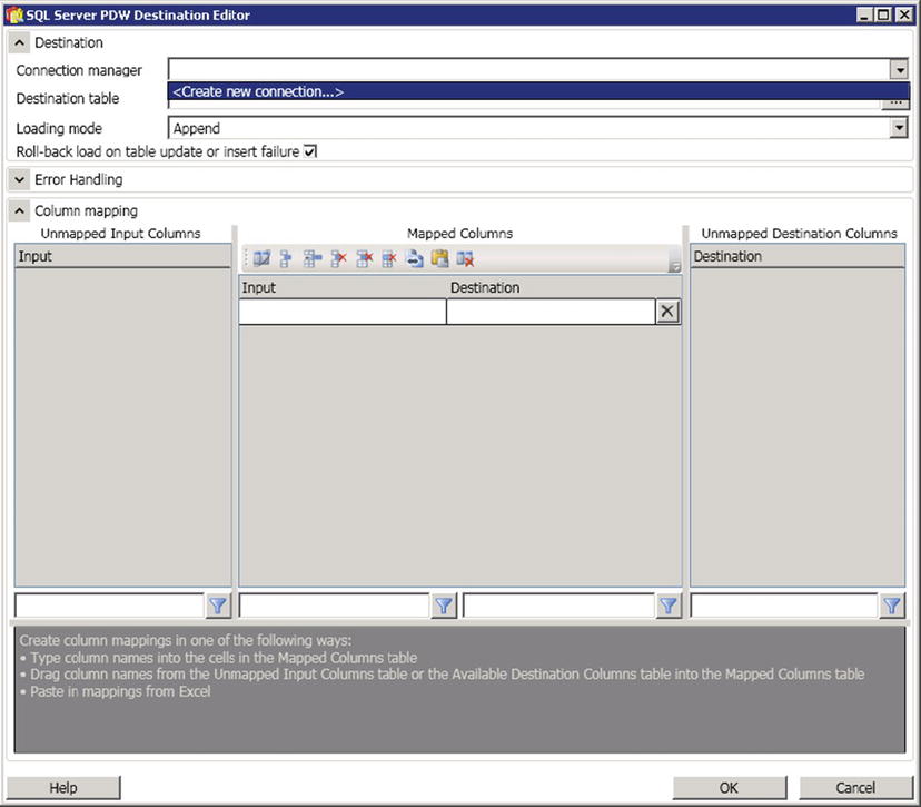
Figure 8-9. The SQL Server PDW Destination Editor
Enter your connection information in the SQL Server PDW Connection Manager Editor using the items described in Table 8-2.
Table 8-2. PDW Connection Information
| Server | The IP address of the Control Node on your appliance (Best practice is to use the clustered IP address to support Control Node failover) |
|---|---|
| User | Your login name for authenticating to the appliance |
| Password | Your login password |
| Destination Database | PDW_Destination_Example |
| Staging Database | StageDB_Example |
Let’s discuss a few best practices relating to this connection information. First, you should specify the IP address of the Control Node cluster instead of the IP address of the active Control Node server. Using the clustered IP address will allow your connection to still resolve without manual intervention in the event of a Control Node failover.
Secondly, although Figure 8-10 shows the sa account being used for authentication, best practice is to use an account other than sa. Doing so will improve the security of your PDW appliance.
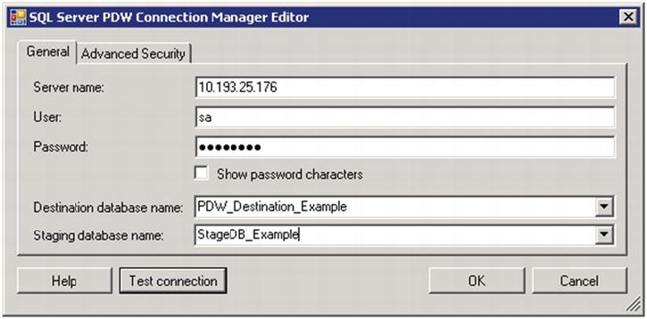
Figure 8-10. The SQL Server PDW Connection Manager Editor
Lastly, as we previously discussed, Microsoft recommends the use of a staging database for data loads. The staging database is selected in the Staging Database Name drop-down. This tells PDW to first load the data to a temporary table in the specified staging database before loading the data into the final destination database. This is optional, but loading directly into the destination database will increase fragmentation.
When you are done, your SQL Server PDW Connection Manager Editor should resemble Figure 8-10. Click on Test Connection to confirm your information was entered correctly, then click OK to return to the SQL Server PDW Destination Editor.
![]() Note If the Staging Database is not specified, SQL Server PDW will perform the load operation directly within the destination database, causing high levels of table fragmentation.
Note If the Staging Database is not specified, SQL Server PDW will perform the load operation directly within the destination database, causing high levels of table fragmentation.
Clicking on the Destination Table field will bring up a modal for Select Destination Table. Click on FactSales, as depicted in Figure 8-11.
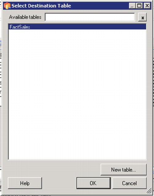
Figure 8-11. The Select Destination Table modal
There are four loading modes available, as listed in Table 8-3.
Table 8-3. The four loading modes
| Append | Inserts the rows at the end of existing data in the destination table. This is the mode you are probably most used to. |
|---|---|
| Reload | Truncates the table before load. |
| Upsert | Performs a MERGE on the destination table, where new data is inserted and existing data is updated. You will need to specify the one or more columns that will be used to join the data on. |
| FastAppend | As its name implies, FastAppend is the fastest way to load data into a destination table. The trade-off is that it does not support rollback; in the case of a failure, you are responsible for removing any partially-inserted rows. FastAppend will also bypass the staging database, causing high levels of fragmentation. |
Let’s take a moment to discuss how to use the modes from Table 8-3 with two common load patterns. If you are performing regular, incremental loads on a large table (say, updating a transactional sales table with the previous day’s orders), you should load the data directly using Append, since no transformations are required. Now let’s say you’re loading the same data, but you plan to instead transform the data and load into a mart before deleting the temporary data. This second example would be better suited to the FastAppend mode. Or, to say it more concisely, use FastAppend any time you are loading into an empty, intermediate working table.
There is one last option we need to discuss. Underneath the Loading Mode is a checkbox for “Roll-back load on table update or insert failure.” In order to understand this option, you need to understand a little about how data is loaded into PDW. When data is loaded using the Append, Reload, or Upsert modes, PDW performs a 2-phase load. In Phase 1, the data is loaded into the staging database. In Phase 2, PDW performs an INSERT/SELECT of the sorted data into the final destination table. By default, data is loaded in parallel on all Compute Nodes, but loaded serially within a Compute Node to each distribution. This is necessary in order to support rollback. Roughly 85-95% of the load process is spent in Phase 1. When “Roll-back load on table update or insert failure” is de-selected, each distribution is loaded in parallel instead of serially during Phase 2. So, in other words, deselecting this option will improve performance but only affects 5-15% of the overall process. Also, deselecting this option removes PDW’s ability to roll back; in the event of a failure during Phase 2, you would be responsible for cleaning up any partially-inserted data.
Because of the potential risk and minimal gain, it is best practice to deselect this option only when loading to an empty table. FastAppend is unaffected by this option because it always skips Phase 2 and loads directly into the final table, which is why FastAppend also does not support rollback.
![]() Tip “Roll-back load on table update or insert failure” is also available in dwloader using the –m option.
Tip “Roll-back load on table update or insert failure” is also available in dwloader using the –m option.
Let’s return to our PDW Destination Editor and select Append in the Loading Mode field. Because our destination table is currently empty, deselect the “Roll-back load on table update or insert failure” option to get a small, risk-free performance boost. Your PDW Destination Editor should now look similar to Figure 8-12.
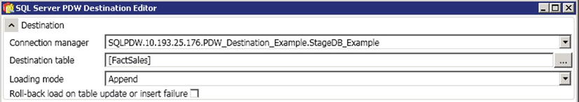
Figure 8-12. The SQL Server PDW Destination Editor
We are almost done with our first Data Flow. All we have left to do is to map our data. Drag the green arrow from the Data Conversion box to the SQL Server PDW Destination box, and then double-click on SQL Server PDW Destination. You should see results like those in Figure 8-13.
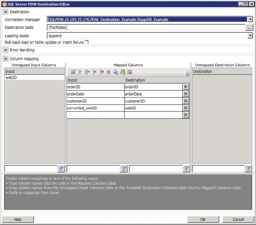
Figure 8-13. The SQL Server PDW Destination Editor
Map your input and destination columns. Make sure to map webID to our transformed converted_webID column. Click OK.
We have now successfully completed our first Data Flow connecting SQL Server to PDW. All we have left is to multi-thread our package.
We have completed our Data Flow for 2010, but we still need to create identical Data Flows for 2011 and 2012. We can do this easily by using copy and paste.
First, click on the Control Flow tab and rename the first Data Flow “SalesMart 2010.” Then, copy and paste “SalesMart 2010” and rename it “SalesMart 2011.”
Double-click on “SalesMart 2011” to return to the Data Flow designer, then double-click on the OLE DB Source. Replace the SQL Command with the code in Listing 8-8.
Listing 8-8. SQL Command for 2011 data
/* Retrieve sales for 2011 */
SELECT
     orderID
     , orderDate
     , customerID
     , webID
FROM PDW_Source_Example.dbo.FactSales
WHERE orderDate = = '2011-01-01'
    AND orderDate < '2012-01-01';
Return to the Control Flow tab and copy the “SalesMart 2010” Data Flow again. Rename it “Sales Mart 2012.” Using the code in Listing 8-9, replace the SQL Command in the OLE DB Source.
Listing 8-9. SQL Command for 2012 Data
/* Retrieve sales for 2012 */
SELECT
         orderID
     , orderDate
     , customerID
     , webID
FROM PDW_Source_Example.dbo.FactSales
WHERE orderDate = = '2012-01-01'
     AND orderDate < '2013-01-01';
We are now ready to execute the package! Press F5 or navigate to Debug ![]() Start Debugging. Your successfully executed package should look similar to Figure 8-14.
Start Debugging. Your successfully executed package should look similar to Figure 8-14.
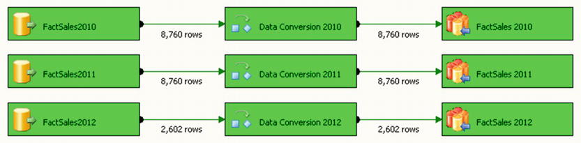
Figure 8-14. The successfully executed package
Summary
We’ve covered a lot of material in this chapter. You have learned about the architecture of Microsoft SQL Server Parallel Data Warehouse (PDW) and some of the differences between SMP and MPP systems. You have learned about different loading methods and discussed how to improve load performance. You have also discovered some best practices along the way. Lastly, you walked through a step-by-step exercise to load data from SQL Server into PDW.