CHAPTER 3        Errors, Faults, and Hazards

3.1 Errors

In the last chapter, we saw that our goal is to avoid service failures. But before considering the engineering techniques that can be used to build computer systems that meet defined dependability requirements, we need to look carefully at the notion of failure again. In essence, before we can deal with failures, we need to answer the question:

We need a general answer to this question, not one that is associated with a specific class of failures or a specific type of system. If we had an answer, that answer would provide the starting point for the engineering necessary to build dependable computer systems.

The answer to this critical question is simple, elegant, and powerful, and the answer provides precisely the starting point we need. The answer to the question is in two parts. A failure occurs when:

•  The system is in an erroneous state.

•  Part of that erroneous state is included in the system’s external state.

where we have the following definition from the taxonomy:

Intuitively, an error is a system state that is not intended and that is one step (or state change) away from a service failure. The elegance and power of this answer to our question lies in its generality and the fact that the answer is based on the notion of system state. We cannot, in general, prevent the error from including part of the external state, and so our basic engineering goal is to avoid errors.

As examples of errors, consider the following situations:

•  A payroll system in which a calculation has been made using an incorrect entry from one of the tax tables. The system state contains a value that is wrong, and, if that value is used for output, the system will have failed.

•  The same payroll system in which the calculation of a certain salary value was performed using an expression in which multiplication rather than division had been used by mistake in the software. Again, the system state contains a value that is wrong, and, if the value is used for output, the system will have failed.

•  An aircraft navigation system in which the data received from the altitude sensor is incorrect because of a break in the cable supplying the data. Further processing by the avionics system using this faulty altitude value, in the autopilot, for example, would probably lead to failure very quickly.

“Error” is a common word in conversation where error is often used as a synonym for mistake. In discussing dependability, error is a state, not an action. Before going on, make sure that you have put your intuitive definition of error to one side and that you use the definition here when thinking about dependability.

FIGURE 3.1 Software defect in a distributed system.

In order to begin the process of engineering dependable systems, we need to look closely at the notion of error, determine how to find all the errors associated with a system, and then determine how errors arise. Fundamentally, achieving dependability comes down to the following process:

•  Identify all of the possible erroneous states into which a system could move.

•  Ensure that either those states cannot be reached or, if they can, the negative effects are known and every effort has been taken to reduce those effects.

Needless to say, this is a difficult challenge, but this process is a useful way to think about what we have to achieve.

3.2 The Complexity of Erroneous States

In computer systems, erroneous states can be very complex. A bug in a program can cause some piece of data to be incorrect, and that data can be used in subsequent calculations so that more (perhaps a lot more) data becomes incorrect. Some of that data can be transmitted to peripherals and other computers, thereby extending the erroneous state to a lot of equipment. All of this can happen quickly and result in a major corruption of the system state.

As an example, consider the system shown in Figure 3.1. In the system shown, three computers are connected over a network, and one computer has a disk and printer connected. Suppose that, because of a software defect, Program 1 generates an erroneous state element that is then sent to programs 2 and 3, and that they then send erroneous data to programs 5 and 7. Finally, program 7 writes erroneous data to the disk and prints some part of that data. The result is the extensive erroneous state, the grey components, shown in Figure 3.2.

FIGURE 3.2 Extensively damaged state in a distributed system from a single bug.

In this example, a failure actually has occurred, because the printed material is part of the external state. Users will have access to the printed material, and so the system is no longer providing the desired service. Whether the users act on the printed material or not does not matter; the system has experienced a service failure.

3.3 Faults and Dependability

3.3.1 Definition of Fault

The reason that the systems we build are not perfectly dependable is the existence of faults. The definition of fault from the taxonomy is:

The first thing to note in this definition is the use of the word cause. When we say “A is a cause of B” what we mean is that A happened and as a result B happened. This notion is the logical notion of implication. Note that the converse does not follow. In other words, the fact that B has happened does not mean that A has happened. In our context here, this means that there could be more than one fault capable of causing a given error.

A fault causing an error seems like a simple notion. If we have an error, surely this means that we can find the fault which caused the error and do something about the fault. In practice, two other words in the definition, adjudged and hypothesized, are important. The words are there to inform us that there might not be a clearly identifiable cause of an error.

This issue is easy to see from the following two examples:

•  Hardware fault.
Suppose that a computer system fails because the hard drive in the system stops working. One might say that the fault is the failed disk drive. But the majority of the disk drive is still working correctly. A closer look reveals that an integrated circuit in the mechanism that controls the motor which moves the read/write head is not working. So one might then conclude that the fault is the failed integrated circuit. But the majority of the integrated circuit is still working correctly. A closer look reveals that a transistor in the integrated circuit is not working. So is the adjudged or hypothesized cause of the error the disk drive, the integrated circuit, or the transistor?

•  Software fault.
Consider a program designed to calculate the tangent of an angle specified in degrees. The software is part of the navigation system for an aircraft. During flight, the crew of the aircraft discovers that the navigation system fails when the aircraft heading is exactly due North. Investigation by software engineers reveals that the problem lies with the tangent software, because the tangent is not defined for 90° and that computation was needed when the heading was due North. One way to fix this problem is to treat 90° as a special case in the tangent software so that the software behaves in an appropriate manner. A second way to fix the problem is to make sure that the software which calls the tangent software never makes the call with the angle set to 90°. So is the adjudged or hypothesized cause of the error the tangent software or the calling software?

As should be clear from these examples, the reason for the difficulty in identifying the fault responsible for a given error is the need to take a systems view of both the notion of error and fault. Recall from the discussion of the term “system” in Section 2.3 (page 30) that a subject system operates within an environment system. The notion of error, no matter how extensive, is associated with the environment system, and the notion of fault is associated with a subject system operating within the environment system. Thus, in the first example above, the error is in the computer system regarded as the environment system for the disk drive. From that perspective, the disk drive is the subject system, and the failed disk drive is the fault.

In a sense, the motto of dependability is “no faults, no problem”. But we do have a problem because in real systems:

More importantly, though, we must keep the definition of service failure from Section 2.6 in mind. Here is the definition again:

Recall that this definition includes the notion of abstract vs. documented requirements. A system that does something other than the intended system function has failed even if the system does the wrong thing correctly. The abstract requirements define the problem to be solved, i.e., the intended function. If the documented requirements and hence the resulting system differ from the abstract requirements, then the differences are likely to lead to service failures. Thus, differences between the abstract requirements and the documented requirements are faults.

3.3.2 Identifying Faults

In order to be able to build dependable systems, we have to gain an understanding of faults and how to deal with them.

Failing to identify a possible fault in a system and failing to deal with that fault while we are designing the system leave the possibility of failure.

In practice, identifying all of the faults to which a system is subject might not be possible. As we shall see in the Chapter 4, the process of identifying fault types is neither formal nor exact, and determining completeness is, at least in part, a matter of experience. Sometimes something gets missed, and sometimes that leads to incidents, accidents, and other forms of loss.

Also in practice, we might choose not to bother to deal with one or more faults that we identify as being possible in a system, because the cost of dealing with the fault is excessive. The cost might require too much equipment or too much analysis, or dealing with the fault might lead to an operating environment that is too restrictive.

3.3.3 Types of Fault

Faults come in three basic types: degradation, design, and Byzantine. The distinction between fault types is of crucial importance. We will use the various fault types extensively in developing our approach to dependability engineering.

Briefly, a degradation fault is a fault that arises because something breaks; a design fault is a fault in the basic design of a system; and a Byzantine fault is a fault for which the effects are seen differently by different elements of the system. These three fault types are discussed in depth in Section 3.5, Section 3.6, and Section 3.7.

Each of these fault types is fundamentally different from the other two, and different techniques are needed to deal with each type. Understanding the characteristics of the three fault types and the differences between them is important. The differences allow us to begin the process of systematically dealing with faults.

Dealing with faults means we have to understand their characteristics, know how to determine the faults about which we need to be concerned in a given system, and know how we will deal with those faults.

3.3.4 Achieving Dependability

We have made a lot of progress toward our goal of being able to develop dependable systems. We have a precise terminology that allows us to document dependability requirements. We know that errors can lead to service failures and therefore that we have to try to prevent them. And, we know that faults are the cause of erroneous states. With this framework in hand, our task becomes one of identifying the faults to which a system is subject and then developing ways of dealing with those faults. This is not a simple task, but now we have a path forward.

3.4 The Manifestation of Faults

A fault in a system is a defective component within the system. If the component is not actively involved in providing service, then the component’s presence, whether faulty or not, is not important. The component cannot affect the state and so the component will not cause an error. This leads to four important definitions:

Active fault:	A fault is active if it causes an error.
Dormant fault:	A fault is dormant if it does not cause an error.
Permanent fault:	A fault is permanent if it is present and remains present.
Transient fault:	A fault is transient if it is present but does not remain present.

The distinction between an active and a dormant fault lies in the effect of the fault on the state. A fault associated with a component, including a software component, need not be of immediate concern provided the component is not being used. Many faults can be present in software, for example, but have no effect if the execution path of the software does not include them.

The distinction between a permanent and a transient fault lies in how we have to deal with the fault. An active transient fault might affect the system state in a way that does not cause a failure, and so designers can exploit the transient nature of the fault.

All of these concepts apply to software. Although software usually fails only on certain inputs, there is a natural tendency to assume that the same software will always fail when given the same input. This is not the case. The reason is that there are numerous sources of non-determinacy in the operation of software, for example:

•  The software might use uninitialized variables, in which case its behavior will depend upon whatever values happened to be in the memory location used for the variables.

•  The software might be concurrent, in which case the scheduling of the individual threads, tasks, or processes will be different on different executions.

•  The software might depend upon hardware- or operating-system-specific information such as timer values, response rates, and sizes of data structures for making decisions.

The idea that the same software might not always fail on the same input led Jim Gray to coin the term Heisenbug (after the physicist Werner Heisenberg, who discovered the Uncertainty Principle) for the associated software faults. For faults that always lead to errors, he coined the term Bohrbug (after the physicist Neils Bohr, who developed the planetary model of the atom) [51]. The practical importance and ways to exploit Heisenbugs are discussed in Section 11.5.

3.5 Degradation Faults

A degradation fault occurs when a component (or maybe more than one) within a system fails. That component used to work but no longer does. The way to think of this is that the component within the system has failed but the system itself has experienced a fault. If we do things right, the system itself will not fail because we can intercede and make sure that the effects of the failed component do not lead to outputs from the system that constitute system failure.

A simple example of a degradation fault can be seen with an incandescent light bulb. When a light bulb is new, the bulb (usually) works, but, as time passes, the filament weakens and eventually breaks. There are many familiar degradation faults in computing systems, including failures of hard disks, power supplies, monitors, keyboards, etc. In each case, the device was working but then failed. Degradation faults are sometimes referred to as wearout faults or random faults.

3.5.1 Degradation Fault Probabilities — The “Bathtub” Curve

A set of components that all seem to be identical will all have different lifetimes. However, if the lifetimes of the members of the set are measured and the mean computed, we will find an average lifetime that is a function of the materials used, the manufacturing process used, the operating environment, the design of the device, and random events.

If the lifetimes of the individual members of the set are measured and the distribution of lifetimes is plotted, the resulting distribution has a well-known shape known as the bathtub curve (see Figure 3.3). The bathtub curve tells us that there are two periods of time when the members of a collection of identical devices tend to fail: shortly after they are put into service and after a long period of service. The former failures are referred to as infant-mortality failures and the latter as end-of-life failures. Failures occur throughout the measurement period but there are two obvious peaks.

Engineers use these two peaks to their advantage in two ways. First, since infant mortality is bound to occur, devices can be put into service by the manufacturer for a period of time at the manufacturer’s facility before delivery. During this period of time, the vast majority of infant mortalities occur. By putting devices into service for a prescribed amount of time before delivery, the manufacturer ensures that the majority of customers will not experience an early failure.

The second use of the bathtub curve is to estimate the MTTF or MTBF of the device. Customers can use this number to determine whether the device will operate for adequate service periods in their application.

In the case of some electronic devices, the failure rate is so low that meaningful population statistics are hard to obtain. Modern integrated circuits, for example, have extraordinary lifetimes if they are operated under conditions of low humidity, low vibration, constant operating temperature (i.e., low thermal stress), and low operating temperature.

3.5.2 An Example of Degradation Faults — Hard Disks

One of the least dependable components of modern systems is the hard disk. Despite this relative lack of dependability, hard disks provide remarkable service. Although the loss of a disk in one of our personal computers is serious for us, having to deal with the prospect of hard-disk failures is very different for operators of large information systems. Such information systems often include storage sub-systems that involve thousands of individual disk units, and on any given day several disks might fail and need to be replaced.

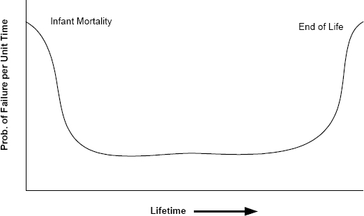
FIGURE 3.3 The bathtub curve showing the variation in failure rate of hardware components over time.

Types of Failure

For disks, there are two important failure effects with which we have to be concerned:

•  An unrecoverable data error in which a read operation fails to return data identical to that which was written.

•  Loss of service from the device in which read and write operations do not complete.

These two types of failure effects¹ can arise with a wide variety of failures within the device, and many of the underlying failures can be intermittent, with complex behavior patterns. These effects lead to difficulty in deciding whether a disk has actually failed. A total lack of response from a disk is fairly clear, but a disk that has to retry read operations and thereby experiences a slight performance loss might: (a) be about to fail permanently, (b) have already lost data that has not been requested, or (c) be suffering from a temporary mechanical flaw.

Rates of Failure

Table 3.1 shows published estimates of failure rates for a number of disks from several manufacturers. These data are only generally indicative of what can be expected from devices like these. A helpful analysis of the complex issue of the performance of desktop machines has been prepared by Cole [29].

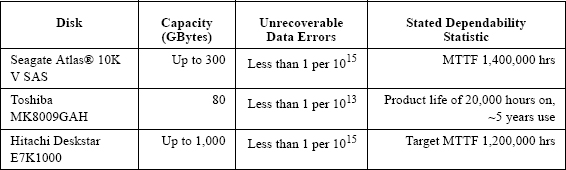
TABLE 3.1. Estimates of disk dependability parameters for typical products from several manufacturers.

Actual failure data of commercial disk drives is hard to come by. Manufacturers are reluctant to publish data about failure rates of their products, and researchers rarely have sufficient samples to study the necessary probability distributions with sufficient accuracy. Another important point about disks is the variety of circumstances in which they operate. Among other things, disks in different personal computers are subject to different rates of use (idle versus operating), different types and severities of mechanical shock, different rates of power cycling (on or off for long periods versus frequent switching), and different temperature and humidity conditions (in a car, near a heating vent, blocked or partially blocked internal fan ducts). With such variety, estimates of rates of failure are of marginal use since they provide little predictive value for any specific disk in operation.

For the use of disks in large information systems, an important study by Schroeder and Gibson [129] provides data from 100,000 disks from four different manufacturers. The observed MTTF for the disks in the study was approximately 1,200,000 hours. But the focus of the work was to look deeper than the simple MTTF, and the detailed results show how many other factors need to be included in models of large numbers of disks in large information systems.

A second important study was carried out by Pinheiro et al. [106]. In that study, more than 100,000 disks from different manufacturers used in the Google File System were monitored. Various disk models were included in the study and the disks were of different ages, because the disk system in the experiment was being maintained and enhanced during the period of study. The results are extensive and detailed, and to a large extent unique because of the large sample size. Some of the results reported include strong correlations between some of the disks’ self-diagnosis data (Self-Monitoring Analysis and Reporting Technology (SMART)) and subsequent failure. Other important results include observation of a lower-than-expected correlation between failure rates and disk temperatures and utilization rates.

Other Concerns About Disks

Further important issues about disks were raised by Gray and van Ingen [52]. In a study of the performance of commodity hardware when a very large amount of data is moved (two petabytes, approximately 10¹⁵ bytes), they observed a variety of system failures that were more significant than the notion of unrecoverable errors in the disk itself. The point is not that unrecoverable errors in the disk are unimportant; they are. The point is that there are other sources of unrecoverable error, such as the cables, the bus, and even the processor and memory, that make the actual rate higher. In addition, unrecoverable errors are not the only source of failure. Gray and van Ingen observed failures of controllers and system reboots.

Other Types of Device

Disks are a good example of the challenge we face when working with computer systems. Many of the issues we have discussed have analogies in other computer-system components. With that in mind, we need to pay attention to two critical points when engineering systems that have to meet specific dependability goals:

•  The role of software in coping with degradation faults in all computer systems is much more elaborate than one might expect. Software at many levels, from the firmware in the disk controller to the operating system, is often called upon to contribute to the goal of dealing with degradation faults.

•  Any effort to estimate the actual dependability of computer systems cannot depend upon simple performance statistics. The actual performance of devices in real application environments is complex and frequently counter-intuitive.

3.6 Design Faults

A design fault is literally a defect in the design of something. An example is a wiring error in a piece of equipment. If a switch is wired backwards, the switch and therefore the equipment of which the switch is part will never work as intended. Nothing changes during the lifetime of the equipment. The switch did not work correctly following manufacture, and the switch will not work correctly at any point during the equipment’s operational lifetime. Unless the switch is repaired, the users of the equipment will have to have a work around for the defective switch whenever they need to use it.

There is no bathtub curve associated with design faults because a device that is subject to a design fault is broken from the outset. This does not mean that the device will not be manufactured or used. Some design faults are unknown at the time of manufacture and end up being present in operational equipment. Design faults do not necessarily manifest themselves in a way that permits their detection during routine testing. This is in complete contrast with degradation faults, where failures will occur over time.

An important thing to note at this point is the following:

This statement usually raises eyebrows and motivates questions such as “Well, what about coding errors?” The problem here is that we are forced to use the word “design” in two different ways — the design phase of the software lifecycle and the type of fault to which software is subject.

The software development lifecycle is shown in Figure 3.4. The lifecycle includes a phase called software “design”, and software engineers consider things like improper use of information hiding and poor choices of abstractions to be defects in the software’s design. Software engineers might not consider defects that are revealed by erroneous outputs from a test case to be defects in the design of their software, because they think of design as one of several specific phases in the software lifecycle. But from the perspective of dependability, all software defects are design faults. We have to be careful to keep in mind that design in the software lifecycle is not the meaning of design in the context of dependability.

Design faults make developing dependable systems challenging. They are faults, and they have to be dealt with. Except for the intentional introduction of a fault to promote malicious interests, design faults are not introduced maliciously. The system’s developers will build the system’s software and undertake all the other design activities using techniques that are meant to produce the “right” product. Where there are defects in a product’s design, in part the defects are the result of unfortunate oversights in the development process.

Determining the design faults to which a system is subject is difficult. To see how significant the problem is, consider the issue of determining the faults in a large software system. Any phase of the software lifecycle could have introduced faults into the software. What are the effects of those faults? The faults could remain dormant for extended periods, because the software component with which they are associated might not be on the execution path. When a fault manifests itself, the software might do anything, including crashing, hanging, generating the wrong output, and generating the correct output but too late. And any of these faults could be Heisenbugs and so even their manifestation would not be certain.

3.7 Byzantine Faults

3.7.1 The Concept

Byzantine faults are faults with completely unpredictable behavior [83]. One might think that the effects of all faults are unpredictable in many ways, and this is certainly true. Rather surprisingly, we all tend to limit the unpredictability that we expect from faults in a way that caused the existence of Byzantine faults to be missed by scientists for a long time.

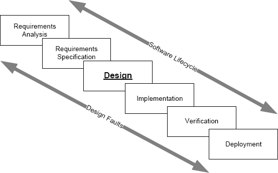
FIGURE 3.4 Design faults can occur at any point in the software lifecycle.

The primary place where we expected predictability is in the effects of a fault when manifested. The problem is that the expectation that all “observers” of a fault will see the same thing, though reasonable, is wrong. Sometimes this expectation is not the case, and then different parts of a system perceive a fault differently.

The basis of this inconsistency in observation is usually a degradation fault. So, in principle, Byzantine faults are not different. In practice, the inconsistency in observation that characterizes Byzantine faults is so important and the treatment of the inconsistency so different, that we are well served by splitting Byzantine faults off as a special case and discussing them separately.

3.7.2 An Example Byzantine Fault

Byzantine faults were first brought to the attention of the scientific community in the development of clock synchronization algorithms. Synchronizing clocks is a vital element of building distributed systems. That the different computers have a view of time that differs by less than a bounded amount is important. If clocks drift at a rate that is less than some threshold, then a set of machines can have clocks that differ from each other by no more than a specific bound if they are synchronized at appropriate intervals.

FIGURE 3.5 Clock synchronization by mid-value selection.

Suppose that we want to synchronize three clocks. An algorithm that we might use is mid-value selection. Each clock sends its current value to the other two, and all three clocks sort the three values they have (their own and the two they received from the other two clocks). By choosing the middle value of the three and setting their times to these values, all three clocks can synchronize to the same value. This process is shown in Figure 3.5.

Now suppose that one clock is faulty and this clock has a time that is very different from the other two. What we would like to happen is for the mid-value selection algorithm to work for us and make sure that the two non-faulty clocks get the same value. This is shown in Figure 3.6. One of the clocks has drifted well outside the expected range; the clock’s value is 60. Yet both of the other clocks synchronize their values correctly as desired.

Now suppose that one of the clocks has a Byzantine fault. By definition, this means that different observers will see its failure differently. This is illustrated in Figure 3.7. The observers are the two non-faulty clocks, and what they see are different times (90 and 105). The result is that the two good clocks now fail to synchronize.

FIGURE 3.6 Clock synchronization by mid-value selection with drifting clock.

3.7.3 Nuances of Byzantine Faults

The idea of a Byzantine fault seems bizarre (or at least Byzantine), and one might be tempted to think that they either do not arise or are rare. Unfortunately, they do arise and cannot be regarded as rare [38].

One might also be tempted to think that the problem lies in the mid-value select algorithm, and that if we could find a different algorithm, all would be well. Again, unfortunately (or fortunately depending upon how you look at the issue) Shostack et. al showed that there is no algorithm that will work [83].

The causes of Byzantine faults are many, and looking at some known causes is instructive if only to get an appreciation of just how subtle they are. Most Byzantine faults arise in data transmission between system components. The causes include:

•  Voltages and clocks operating at marginal levels.

•  Faulty connectors or other mechanical elements of transmission paths.

•  Electrical noise.

•  Other forms of radiation such as cosmic rays.

Some Byzantine faults arise within digital electronics as a result of voltages that lie between logic 1 and logic 0 [38]. Where circuits are operated with imprecise voltages, the logic outputs can vary between logic 0 and logic 1, and a single output that is supplied to different parts of the circuit can end up being different at the different destinations.

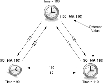
FIGURE 3.7 Clock synchronization failure with a clock experiencing a Byzantine fault.

3.8 Component Failure Semantics

We are not quite finished with the notion of a fault even though we have looked at the three basic fault types. The problem we now need to deal with is to understand what happens to a component when that component fails. More specifically, we need to know what the component’s interfaces will look like and the extent of the damage to which the fault leads. The interface that the component presents after failure and the damage outside the component are referred to as the component failure semantics.

3.8.1 Disk Drive Example

To understand the need for a precise statement of component failure semantics, consider what happens to a disk drive when the drive fails. Disk failures typically result in the disk contents being unreadable, at least partially. Other than loss of data, the failure of a disk drive rarely has much of an effect. Thus, the failure semantics of a disk drive are usually restricted to a loss of data. For purposes of analysis, assuming that all of the stored data is lost is probably best, although that might not always be the case.

Suppose however, that we had to worry about failing disk drives that do not lose data but instead started supplying data that was corrupted in some way. The data supplied on a read request would not be that which was requested by the operating system but was, instead, something that was the wrong information (from a different file, for example) or was random but reasonable looking data. Such a situation would be catastrophic because the data would be supplied to the application, and the application might act on the data without realizing that the data was not that which was needed.

When a disk crashes and all the data is lost, we generally think of this as being catastrophic, and, if there is no backup, the disk crash probably is catastrophic. But the fact that we cannot get any data tells us immediately that the disk has failed. With that knowledge, we can be sure that applications will not operate with corrupt data, a situation that would more than likely be much worse than a total loss of data. Knowing how a component will fail allows us to protect systems from the effects of the component failure. If we do not know, then there is a good chance that we could do nothing to protect the rest of the computer system from the component failure.

Just as with a component’s interface, knowing the extent of the damage that might result from a component failure is important. In the case of a disk drive, for example, there is little likelihood that the disk will affect data stored on a different device. Violent mechanical failure of a disk drive in which nearby components are damaged physically is also unlikely. So the damage to the state that results from a disk failure is limited to the disk’s own contents.

3.8.2 Achieving Predictable Failure Semantics

When examining components in order to determine what faults might arise, we have to determine not just what the faults are but also the component failure semantics. This determination is sufficiently important that components are frequently designed to have well-defined failure semantics. Achieving well-defined failure semantics might just involve careful selection of design techniques or include explicit additions to the design that help to define the failure semantics. Parity in memory is an example of an explicit addition. By including a parity bit, a single bit error in the data can be detected. Thus, for a failure of a memory component in which a single bit is lost, the failure semantics are made detectable and thereby actionable by the provision of a parity mechanism.

In the case of a disk drive, error detecting codes are added extensively in data storage and transmission to allow corrupt data to be detected. The types of failure to which the disk is subject help to define the types of codes. In some cases, disks suffer burst errors and in others random bits are lost. Different codes are added to allow the detection of each of the different anticipated types of failure. Without such codes, data could become corrupted and the failure semantics would be arbitrary. With the error codes present, a disk’s failure semantics can be made precise and properly signaled, raising an interrupt, for example.

3.8.3 Software Failure Semantics

Unfortunately, the well-defined and predictable damage that we achieve with disk drives and most other hardware components is usually not possible for software components. As we saw in Section 3.2, when a software component fails, propagation of the immediate erroneous state is possible, and the erroneous state could be acted upon so as to damage the state extensively outside of the failed software component. By passing elements of an erroneous state to other programs and devices, a failed software component can cause damage that is essentially arbitrary.

We noted in Section 3.8.2 that the creation of manageable failure semantics for a disk drive requires the addition of explicit mechanisms, often including error-detecting codes, to help ensure that the failure semantics are predictable. Could we do the same thing for software? The answer to this question is both “yes” and “no”. Including checks in software to ascertain whether the results being produced are as they should be is certainly possible. The problem is that such checks are far too weak to allow them to be trusted under all circumstances. Unlike disks, where essentially all types of failure to which the disk is subject can be both predicted and checked for, software is so complex that there is no hope of doing as well with software as we can with disks and similar devices. We will examine software error detection in detail in Chapter 11 as part of our discussion of fault tolerance.

3.9 Fundamental Principle of Dependability

As we saw in Section 3.3, faults are the central problem in dependability. Thus, in order to improve the dependability of computing systems, we have to get the right requirements and then deal with faults in the system as constructed. If we can make the improvement in dependability sufficient that the resulting system meets its dependability requirement, then we achieved our most important goal.

Requirements engineering is the process of determining and documenting the requirements for a system. Requirements engineering is a major part of computer system development and the subject of textbooks, at least one journal, and a conference series. We do not discuss requirements engineering further, because the topic is complex and discussed widely elsewhere.

There are four approaches to dealing with faults:

•  Avoidance	-  Section 3.9.1
•  Elimination	-  Section 3.9.2
•  Tolerance	-  Section 3.9.3
•  Forecasting	-  Section 3.9.4

If we were able to predict all of the faults that can occur in systems and combine the results with these four approaches in various ways, we could produce an engineering roadmap that will allow us to either meet the dependability requirements for a given system or show that the dependability requirements were sufficiently extreme that they were unachievable with the available engineering. This idea is central to our study of dependable systems, and so I refer to the idea as the Fundamental Principle of Dependability²:

This principle provides a focus and a goal for our engineering. In all that we do, the role of our activities can be assessed and compared with other possible activities by appealing to this principle. The principle combines the two major issues we face:

•  We need to have a high level of assurance that the documented specification is a solution to the problem defined by the abstract requirements, i.e., that faults in the documented specification (and by implication the documented requirements) have been dealt with appropriately.

•  We need to have a high level of assurance that the system as implemented is a refinement of the solution as stated in the documented specification, i.e., that the faults in the system as built have been dealt with appropriately.

In this section, we examine each of the four approaches to dealing with faults so as understand what is involved in each one. In later chapters, we explore the various techniques available for effecting each approach.

3.9.1 Fault Avoidance

Fault avoidance means, quite literally, avoiding faults. If we can build systems in which faults are absent and cannot arise, we need to do nothing more. From a software perspective, fault avoidance is our first and best approach to dealing with faults, because the alternatives are not guaranteed to work and can have substantial cost. Fault avoidance must always be the approach that we attempt first.

Degradation fault avoidance might seem like an unachievable goal, but it is not. There are many techniques that allow the rate of degradation faults to be reduced to a level at which they occur so infrequently in practice that they can be ignored. For design faults, analysis and synthesis techniques exist that allow us to create designs in some circumstances and know that there are no design faults. Finally, architectural techniques exist that allow us to limit and sometimes eliminate the possibility of Byzantine faults.

All of the techniques that can help us to achieve fault avoidance have limited capability, applicability, and performance, and so we cannot use them exclusively. But remembering the possibility of fault avoidance and seeking out ways to avoid faults in any development are important.

3.9.2 Fault Elimination

If we cannot avoid faults, then the next best thing is to eliminate them from the system in which they are located before the system is put into use. Although not as desirable as fault avoidance, fault elimination is still highly beneficial.

A simple example of degradation fault elimination is the treatment of infant mortality. By operating hardware entities before shipment, manufacturers are looking for those entities that would normally fail early in the field.

A simple example of design fault elimination is software testing. By testing a piece of software, developers are looking for faults in the software so that they can be removed before the software is deployed.

3.9.3 Fault Tolerance

If we can neither avoid nor eliminate faults, then faults will be present in systems during operational use. They might be degradation faults that arise during operation or design faults. If a fault does not manifest itself, i.e., the fault is dormant, then the fault has no effect. Fault tolerance is an approach that is used in systems for which either: (a) degradation faults are expected to occur at a rate that would cause an unacceptable rate of service failure or (b) complete avoidance or elimination of design faults was not possible and design faults were expected to remain in a system.

3.9.4 Fault Forecasting

Finally, if we cannot deal with a fault by avoidance, elimination, or tolerance, we have to admit that untreated faults will be present during operation, and we must try to forecast the effects of the fault. By doing so we are able to predict the effect of the fault on the system and thereby make a decision about whether the system will meet its dependability requirements.

3.10 Anticipated Faults

The fundamental principle of dependability tells us that one thing we have to do in order to meet our dependability requirements is to determine all of the faults to which a system is subject. This goal is easily stated but hard to do, and the goal leads to the notion of anticipated faults.

An anticipated fault is one that we have identified as being in the set to which a system is subject. We know that the fault might arise, and so we have anticipated the fault.

If our techniques for determining the faults to which a system is subject were perfect, we would be done. But these techniques are not perfect. The result is that some faults will not be anticipated. Because they are unanticipated, such faults will not be handled in any type of predictable way, and so their effect on the system of interest is unknown.

Unanticipated faults are the cause of most but not all system failures. There are two reasons why they are not responsible for all system failures:

•  Some system failures result from anticipated faults that were not dealt with in any way. Their effects and probability of occurrence were examined using fault forecasting, and the system designers decided that no treatment was warranted.

•  Some system failures result from failures of fault tolerance mechanisms designed to cope with the effects of anticipated faults.

In summary, our goal is to eliminate unanticipated faults and to make sure that all anticipated faults are dealt with adequately. In order to reach this goal, we need a systematic way of identifying and therefore anticipating faults. The approach we will follow to perform this identification is to first identify the hazards to which the system is subject and then identify the faults that could lead to those hazards.

3.11 Hazards

3.11.1 The Hazard Concept

A hazard is a system state. The notion of hazard arises primarily in the field of safety. Informally, a hazard is a system state that could lead to catastrophic consequences, i.e., a system state that could lead to a violation of safe operation.

The word “hazard” has various meanings in everyday speech, and hazard is another example of why careful attention to definitions is so important. Here is the definition from the taxonomy:

Closely related to the notion of hazard is the notion of an accident:

An accident results when a system is in a hazardous state and a change in the operating environment occurs that leads to a loss event.

A system being in a hazardous state does not necessarily mean that an accident will result. The system could stay in a hazardous state for an arbitrary length of time, and, provided there is no change in the environment that leads to a loss, there will be no accident. Similarly, a system could enter and exit a hazardous state many times without an accident occurring. Clearly, however, we cannot rely on systems in hazardous states remaining accident free.

Some examples of hazards and accidents are the following:

•  An elevator shaft with a door open but with no elevator car present.
For an accident to occur, an environmental circumstance has to arise, e.g., a person walks through the open door unaware of the state.

•  A gate at a railway crossing that fails up.
If a vehicle crosses the track as a train approaches because the driver believes, incorrectly, that proceeding is safe, a collision is likely to occur.

•  A failed automobile anti-lock braking system (ABS) that does not alert the driver to the lack of anti-lock braking capability.
The car could skid and crash if the driver applies the brakes on a slippery surface expecting that the ABS would act to facilitate proper braking.

•  A failed nuclear reactor shutdown system that does not alert the reactor operators to the lack of monitoring capability.
With the shutdown system non-operational, the operators should shut down the reactor immediately. Not doing so is not dangerous in and of itself, but, if an automatic shutdown becomes necessary, the shutdown will not occur and the result could be catastrophic.

•  Crucial information such as credit-card or social-security numbers stored in a publicly accessible file.
The confidentiality and integrity of the data would not necessarily be compromised if information were available to unauthorized users. But should the availability of the data become known to individuals with malicious intent, the result could be catastrophic.

Note that all of the hazards in this list are likely to arise because of defects in computer systems. Instances of all of them have occurred at various times. Hazards, therefore, have a significant impact on all phases of the software lifecycle.

A system can enter a hazardous state for two reasons:

The system design includes states that are hazardous. In this case, the cause is incomplete analysis by the system’s original designers. An example of such a design is a toy with a separable part that could choke a child.

The failure of some component causes the system to enter a hazardous state. In this case, the cause is the component failure. An example of such a failure is the loss of brake hydraulic fluid in a car.

These two reasons are equally important. The first is concerned with the basic design of a system, and the second with states that might arise because of the manifestation of faults. This book is concerned mainly with the latter.

3.11.2 Hazard Identification

In developing systems for which safety is an important dependability requirement, hazards are the states we have to avoid. Provided all the hazards have been identified, by avoiding them, we can be sure that there will be no catastrophic consequences of system operation. In order to arrange for a specific system to avoid hazards, we need to know what hazards can arise. Only then can we seek ways of eliminating them as possible states. The process of identifying and assessing hazards is hazard identification.

Hazard identification and the subsequent analysis of the hazards is a complex and sophisticated process that is conducted primarily by engineers in the associated application domain. In domains such as nuclear power engineering, the determination of what constitutes a hazard is based on a wide variety of inputs. A lot of undesirable states can arise but determining those that are hazards requires analysis by a range of experts. Many industries have developed standards to guide the hazard-analysis process, for example, the nuclear power industry [7].

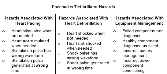
FIGURE 3.8 Some of the hazards associated with a pacemaker/defibrillator.

Our interest is in computer systems, and, in many cases, the computer systems that we build will be responsible for the prevention of hazards. We, as software engineers, have to be aware of hazard identification and analysis, because the results of the analysis will frequently appear in the computer system’s requirements. However, primary responsibility for hazard analysis does not lie with the computer or software engineer.

As an example of what is involved in hazard identification, consider a hypothetical implantable combined pacemaker and defibrillator. The only significant accident with which the designers of such a device have to be concerned is patient injury. Clearly, for a device like this, injury could lead to death.

The hazards for a combined pacemaker and defibrillator break down conveniently into three categories, as shown in Figure 3.8 — those associated with heart pacing, those associated with heart defibrillation, and those associated with equipment management. In each category, there are four hazards of which we have to take note. The first two categories are concerned with fairly obvious treatment failures. The third category concerns equipment management and is concerned with the possibility of things like a detached lead going unnoticed or the backup analog pacing circuit becoming unavailable and this situation not being detected.

3.11.3 Hazards and Faults

Note carefully that a hazard is an error, i.e., erroneous state. Recall that a fault is the adjudged cause of an error, and this provides the link between faults and hazards. In order to avoid a hazard, we need to identify the faults that might cause the hazard and make sure that each fault has been suitably treated. In Chapter 4, we will examine ways of identifying the faults that might cause a given hazard. Combining this process of fault identification with hazard analysis, we finally have a comprehensive way of identifying the faults to which a system is subject.

Although the notion of hazard is most commonly used in the field of safety, we can exploit the notion generally to help define a systematic approach to dependability engineering. We will treat the notion of hazard as any state that we would like to avoid rather than just those with catastrophic consequences. As we shall see in Section 4.2 on page 104, treating the state in which a component has failed as a hazard is useful even if that state could not lead to an accident in the sense of Section 3.11.1. The component might be a computer system or part of one.

3.12 Engineering Dependable Systems

We can now bring together all the various ideas we have explored in this chapter and create an overall process for engineering dependable systems. For any system, there are two sets of requirements: the functional requirements and the dependability requirements, and these two sets of requirements are used to guide the system design process. Both are needed because the system has to supply the required functionality and do so with the required dependability.

From the fundamental principle of dependability, we know that our engineering task is to anticipate the faults to which a system is subject and to deal with each in a manner that ensures that the system meets its dependability goal to the extent possible.

Hazards are states that we want to avoid, and we will anticipate all the faults to which a system is subject by identifying all of the hazards that might arise and then determining the faults that could lead to each hazard.

Next, for each fault that we have identified, i.e., anticipated, we will determine a suitable approach to dealing with that fault using one of the four available techniques: avoidance, elimination, tolerance, or forecasting.

Finally, we will assess the dependability of the resulting system as best we can, and, if the assessment indicates the possibility of not meeting the dependability requirements, we will cycle through the process again, beginning with a system redesign.

This leads us to a dependability engineering process that is illustrated in Figure 3.9. The overall flow of engineering activities is:

•  Define the system’s functional requirements.

•  Define the system’s dependability requirements.

•  Determine the hazards to which the system is subject based on the functional requirements.

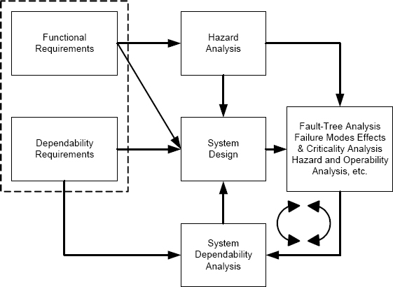
FIGURE 3.9 The dependability engineering process.

•  Design the system to meet both the functional and the dependability requirements.

•  For each hazard, determine the faults that could lead to that hazard. This analysis is based on a variety of different information, but the goal is to obtain the complete list of anticipated faults.

•  For each anticipated fault, determine a means of dealing with the fault. Each fault will be dealt with by avoidance, elimination, tolerance, or forecasting.

•  Assess the resulting system to determine whether the system’s dependability goals will be met. If the dependability requirements will not be met, then the system has to be redesigned and the assessment process repeated.

The assessment step might lead to multiple iterations of the process if the system design does not necessarily lead to the dependability requirements being met. For example, if the dependability assessment shows that the rate of hardware failure will lead to service failures from the complete system that are beyond the rate defined to be acceptable, the hardware will have to be redesigned and the assessment repeated.

Our discussion in this section is a high-level overview intended to act as something of a road map. Dependability engineering of a modern software-intensive system is a complicated process that expands on this road map considerably. However, underneath the detail, the principles are the same.

Key points in this chapter:

 

Exercises

1.  Carefully and succinctly explain why a mistake in the implementation source code of a piece of software is referred to as a design fault rather than an implementation fault.

2.  Explain the difference between a hazard and an accident and illustrate your answer using examples from a system with which you are familiar.

3.  For the ABS system described in Exercise 17 in Chapter 2:

(a) Determine the set of hazards that can arise.

(b) Identify the degradation faults that need to be anticipated.

(c) Identify the design faults that need to be anticipated.

4.  For each degradation fault you identified in Exercise 3(b), determine whether software functionality might be used to help deal with the fault when the fault is manifested. For those where this is the case, state informally what you think the software might be required to do.

5.  Consider the pharmacy information system described in Exercise 15 in Chapter 2.

(a) List the dependability attribute or attributes that need to considered for this system and for each explain why each attribute is important.

(b) For one of the attributes listed in part (a), carefully define a possible requirement statement for that dependability attribute for this system.

6.  Identify three major hazards that the pharmacy information system faces.

7.  In August 2005, a serious incident occurred aboard a Boeing 777 flying over Australia. The official report of the incident is available from the Australian Transport Safety Bureau [11].

(a) For the B777 incident, document the failed component combinations that were deemed safe for flight.

(b) For the B777 incident, clearly the aircraft was in a hazardous state. What where the characteristics of the state that made the state hazardous?

(c) For the B777 incident, how and when did the hazardous state arise?

8.  For one of the hazards that you identified in Exercise 6, indicate how you would go about calculating the associated cost of failure in dollars.

9.  A robotic surgery system is a machine tool designed for use in an operating room to assist surgeons in joint-replacement surgery. The system operates by cutting bone to a specific shape that accepts a joint-replacement implant. The system is illustrated in the following figure:

     The system is much more precise than human surgeons and the benefits to the patient of robotic surgery are tremendous. Needless to say, the cutting process is complex and computer controlled. The cutting tool moves in an elaborate pattern to shape the bone. The location of the patient and all the robot equipment is determined precisely by a 3D tracking system. Obviously the concern that the robot’s developers have is the possibility of the robot cutting something that it should not, for example, if the software calculated the wrong direction or distance for the cut. In an effort to prevent this, the cutting edge of the tool is monitored by a second computer system that computes the tool’s planned track separately. The primary computer and the tracking computer have to agree in order for the robot to proceed. For the robotic surgery system:

(a) Identify the hazards to which you think the system is subject.

(b) Identify the degradation faults to which you think the system’s cutting head might be subject.

(c) Identify possible Byzantine faults that might occur in the system.