Chapter 2. The Meaning of Programs
Don’t think, feel! It is like a finger pointing away to the moon. Don’t concentrate on the finger or you will miss all that heavenly glory.
Programming languages, and the programs we write in them, are fundamental to our work as software engineers. We use them to clarify complex ideas to ourselves, communicate those ideas to each other, and, most important, implement those ideas inside our computers. Just as human society couldn’t operate without natural languages, so the global community of programmers relies on programming languages to transmit and implement our ideas, with each successful program forming part of a foundation upon which the next layer of ideas can be built.
Programmers tend to be practical, pragmatic creatures. We often learn a new programming language by reading documentation, following tutorials, studying existing programs, and tinkering with simple programs of our own, without giving much thought to what those programs mean. Sometimes the learning process feels a lot like trial and error: we try to understand a piece of a language by looking at examples and documentation, then we try to write something in it, then everything blows up and we have to go back and try again until we manage to assemble something that mostly works. As computers and the systems they support become increasingly complex, it’s tempting to think of programs as opaque incantations that represent only themselves and work only by chance.
But computer programming isn’t really about programs, it’s about ideas. A program is a frozen representation of an idea, a snapshot of a structure that once existed in a programmer’s imagination. Programs are only worth writing because they have meaning. So what connects code to its meaning, and how can we be more concrete about the meaning of a program than saying “it just does whatever it does”? In this chapter, we’re going to look at a few techniques for nailing down the meanings of computer programs and see how to bring those dead snapshots to life.
The Meaning of “Meaning”
In linguistics, semantics is the study of the connection between words and their meanings: the word “dog” is an arrangement of shapes on a page, or a sequence of vibrations in the air caused by someone’s vocal cords, which are very different things from an actual dog or the idea of dogs in general. Semantics is concerned with how these concrete signifiers relate to their abstract meanings, as well as the fundamental nature of the abstract meanings themselves.
In computer science, the field of formal semantics is concerned with finding ways of nailing down the elusive meanings of programs and using them to discover or prove interesting things about programming languages. Formal semantics has a wide spectrum of uses, from concrete applications like specifying new languages and devising compiler optimizations, to more abstract ones like constructing mathematical proofs of the correctness of programs.
To completely specify a programming language, we need to provide two things: a syntax, which describes what programs look like, and a semantics,[2] which describes what programs mean.
Plenty of languages don’t have an official written specification, just a working interpreter or compiler. Ruby itself falls into this “specification by implementation” category: although there are plenty of books and tutorials about how Ruby is supposed to work, the ultimate source of all this information is Matz’s Ruby Interpreter (MRI), the language’s reference implementation. If any piece of Ruby documentation disagrees with the actual behavior of MRI, it’s the documentation that’s wrong; third-party Ruby implementations like JRuby, Rubinius, and MacRuby have to work hard to imitate the exact behavior of MRI so that they can usefully claim to be compatible with the Ruby language. Other languages like PHP and Perl 5 share this implementation-led approach to language definition.
Another way of describing a programming language is to write an official prose specification, usually in English. C++, Java, and ECMAScript (the standardized version of JavaScript) are examples of this approach: the languages are standardized in implementation-agnostic documents written by expert committees, and many compatible implementations of those standards exist. Specifying a language with an official document is more rigorous than relying on a reference implementation—design decisions are more likely to be the result of deliberate, rational choices, rather than accidental consequences of a particular implementation—but the specifications are often quite difficult to read, and it can be very hard to tell whether they contain any contradictions, omissions, or ambiguities. In particular there’s no formal way to reason about an English-language specification; we just have to read it thoroughly, think about it a lot, and hope we’ve understood all the consequences.
Note
A prose specification of Ruby 1.8.7 does exist, and has even been accepted as an ISO standard (ISO/IEC 30170).[3] MRI is still regarded as the canonical specification-by-implementation of the Ruby language, although the mruby project is an attempt to build a lightweight, embeddable Ruby implementation that explicitly aims for compliance with the ISO standard rather than MRI compatibility.
A third alternative is to use the mathematical techniques of formal semantics to precisely describe the meaning of a programming language. The goal here is to be completely unambiguous, as well as to write the specification in a form that’s suited to methodical analysis, or even automated analysis, so that it can be comprehensively checked for consistency, contradiction, or oversight. We’ll look at these formal approaches to semantic specification after we’ve seen how syntax is handled.
Syntax
A conventional computer program is a long string of characters. Every programming language comes with a collection of rules that describe what kind of character strings may be considered valid programs in that language; these rules specify the language’s syntax.
A language’s syntax rules allow us to distinguish potentially valid programs like y = x + 1 from nonsensical ones like >/;x:1@4. They also provide useful information about how to read ambiguous
programs: rules about operator precedence, for example, can automatically determine that
1 + 2 * 3 should be treated as though it had been written
as 1 + (2 * 3), not as (1 + 2) *
3.
The intended use of a computer program is, of course, to be read by a computer, and reading programs requires a parser: a program that can read a character string representing a program, check it against the syntax rules to make sure it’s valid, and turn it into a structured representation of that program suitable for further processing.
There are a variety of tools that can automatically turn a language’s syntax rules into a parser. The details of how these rules are specified, and the
techniques for turning them into usable parsers, are not the focus of this chapter—see Implementing Parsers for a quick overview—but overall, a parser should read a
string like y = x + 1 and turn it into an abstract syntax tree (AST), a representation of the
source code that discards incidental detail like whitespace and focuses on the hierarchical
structure of the program.
In the end, syntax is only concerned with the surface appearance of programs, not with their meanings. It’s possible for a program to be syntactically
valid but not mean anything useful; for example, it might be that the program y = x + 1 doesn‘t make sense on its own because it doesn’t say
what x is beforehand, and the program z = true + 1 might turn out to be broken when we run it because
it’s trying to add a number to a Boolean value. (This depends, of course, on other properties
of whichever programming language we’re talking about.)
As we might expect, there is no “one true way” of explaining how the syntax of a programming language corresponds to an underlying meaning. In fact there are several different ways of talking concretely about what programs mean, all with different trade-offs between formality, abstraction, expressiveness, and practical efficiency. In the next few sections, we’ll look at the main formal approaches and see how they relate to each other.
Operational Semantics
The most practical way to think about the meaning of a program is what it does—when we run the program, what do we expect to happen? How do different constructs in the programming language behave at run time, and what effect do they have when they’re plugged together to make larger programs?
This is the basis of operational semantics, a way of capturing the meaning of a programming language by defining rules for how its programs execute on some kind of device. This device is often an abstract machine: an imaginary, idealized computer that is designed for the specific purpose of explaining how the language’s programs will execute. Different kinds of programming language will usually require different designs of abstract machine in order to neatly capture their runtime behavior.
By giving an operational semantics, we can be quite rigorous and precise about the purpose of particular constructs in the language. Unlike a language specification written in English, which might contain hidden ambiguities and leave important edge cases uncovered, a formal operational specification will need to be explicit and unambiguous in order to convincingly communicate the language’s behavior.
Small-Step Semantics
So, how can we design an abstract machine and use it to specify the operational semantics of a programming language? One way is to imagine a machine that evaluates a program by operating on its syntax directly, repeatedly reducing it in small steps, with each step bringing the program closer to its final result, whatever that turns out to mean.
These small-step reductions are similar to the way we are taught in school to evaluate algebraic expressions. For example, to evaluate (1 × 2) + (3 × 4), we know we should:
Perform the left-hand multiplication (1 × 2 becomes 2) and reduce the expression to 2 + (3 × 4)
Perform the right-hand multiplication (3 × 4 becomes 12) and reduce the expression to 2 + 12
Perform the addition (2 + 12 becomes 14) and end up with 14
We can think of 14 as the result because it can’t be reduced any further by this process—we recognize 14 as a special kind of algebraic expression, a value, which has its own meaning and doesn’t require any more work on our part.
This informal process can be turned into an operational semantics by writing down formal rules about how to proceed with each small reduction step. These rules themselves need to be written in some language (the metalanguage), which is usually mathematical notation.
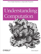
In this chapter, we’re going to explore the semantics of a toy programming language—let’s call it Simple.[4] The mathematical description of Simple’s small-step semantics looks like this:
Mathematically speaking, this is a set of inference rules that defines a reduction relation on Simple’s abstract syntax trees. Practically speaking, it’s a bunch of weird symbols that don’t say anything intelligible about the meaning of computer programs.
Instead of trying to understand this formal notation directly, we’re going to investigate how to write the same inference rules in Ruby. Using Ruby as the metalanguage is easier for a programmer to understand, and it gives us the added advantage of being able to execute the rules to see how they work.
Warning
We are not trying to describe the semantics of Simple by giving a “specification by implementation.” Our main reason for describing the small-step semantics in Ruby instead of mathematical notation is to make the description easier for a human reader to digest. Ending up with an executable implementation of the language is just a nice bonus.
The big disadvantage of using Ruby is that it explains a simple language by using a more complicated one, which perhaps defeats the philosophical purpose. We should remember that the mathematical rules are the authoritative description of the semantics, and that we’re just using Ruby to develop an understanding of what those rules mean.
Expressions
We’ll start by looking at the semantics of Simple expressions. The rules will operate on the abstract syntax of these expressions, so we need to be able to represent Simple expressions as Ruby objects. One way of doing this is to define a Ruby class for each distinct kind of element from Simple’s syntax—numbers, addition, multiplication, and so on—and then represent each expression as a tree of instances of these classes.
For example, here are the definitions of Number, Add, and Multiply classes:
classNumber<Struct.new(:value)endclassAdd<Struct.new(:left,:right)endclassMultiply<Struct.new(:left,:right)end
We can instantiate these classes to build abstract syntax trees by hand:
>>Add.new(Multiply.new(Number.new(1),Number.new(2)),Multiply.new(Number.new(3),Number.new(4)))=> #<struct Addleft=#<struct Multiplyleft=#<struct Number value=1>,right=#<struct Number value=2>>,right=#<struct Multiplyleft=#<struct Number value=3>,right=#<struct Number value=4>>>
Note
Eventually, of course, we want these trees to be built automatically by a parser. We’ll see how to do that in Implementing Parsers.
The Number, Add, and Multiply classes inherit Struct’s generic
definition of #inspect, so the
string representations of their instances in the IRB console contain a
lot of unimportant detail. To make the content of an abstract syntax
tree easier to see in IRB, we’ll override #inspect on each class[5] so that it returns a custom string
representation:
classNumberdefto_svalue.to_senddefinspect"«#{self}»"endendclassAdddefto_s"#{left}+#{right}"enddefinspect"«#{self}»"endendclassMultiplydefto_s"#{left}*#{right}"enddefinspect"«#{self}»"endend
Now each abstract syntax tree will be shown in IRB as a short string of Simple source code, surrounded by «guillemets» to distinguish it from a normal Ruby value:
>>Add.new(Multiply.new(Number.new(1),Number.new(2)),Multiply.new(Number.new(3),Number.new(4)))=> «1 * 2 + 3 * 4»>>Number.new(5)=> «5»
Warning
Our rudimentary #to_s implementations don’t take
operator precedence into account, so sometimes their output is incorrect with respect to
conventional precedence rules (e.g., * usually binds
more tightly than +). Take this abstract syntax tree,
for example:
>>Multiply.new(Number.new(1),Multiply.new(Add.new(Number.new(2),Number.new(3)),Number.new(4)))=> «1 * 2 + 3 * 4»
This tree represents «1 * (2 + 3) *
4», which is a different expression (with a different
meaning) than «1 * 2 + 3 * 4»,
but its string representation doesn’t reflect that.
This problem is serious but tangential to our discussion of semantics. To keep things simple, we’ll temporarily ignore it and just avoid creating expressions that have an incorrect string representation. We’ll implement a proper solution for another language in Syntax.
Now we can begin to implement a small-step operational semantics by defining methods that perform reductions on our abstract syntax trees—that is, code that can take an abstract syntax tree as input and produce a slightly reduced tree as output.
Before we can implement reduction itself, we need to be able to
distinguish expressions that can be reduced from those that can’t.
Add and Multiply expressions are always
reducible—each of them represents an operation, and can be turned into
a result by performing the calculation corresponding to that
operation—but a Number expression
always represents a value, which can’t be reduced to anything
else.
In principle, we could tell these two kinds of expression apart with a single #reducible? predicate that returns true or false depending on the class of
its argument:
defreducible?(expression)caseexpressionwhenNumberfalsewhenAdd,Multiplytrueendend
Note
In Ruby case statements,
the control expression is matched against the cases by calling each
case value’s #=== method with the
control expression’s value as an argument. The implementation of
#=== for class objects checks to
see whether its argument is an instance of that class or one of its
subclasses, so we can use the case
syntax to match an
object against a class.object when
classname
However, it’s generally considered bad form to write code like this in an
object-oriented language;[6] when the behavior of some operation depends upon the
class of its argument, the typical approach is to implement each
per-class behavior as an instance method for that class, and let the
language implicitly handle the job of deciding which of those methods
to call instead of using an explicit case statement.
So instead, let’s implement separate #reducible? methods for Number, Add, and Multiply:
classNumberdefreducible?falseendendclassAdddefreducible?trueendendclassMultiplydefreducible?trueendend
This gives us the behavior we want:
>>Number.new(1).reducible?=> false>>Add.new(Number.new(1),Number.new(2)).reducible?=> true
We can now implement reduction for these expressions; as above, we’ll do this by
defining a #reduce method for Add and Multiply. There’s no need to
define Number#reduce, since numbers can’t be reduced,
so we’ll just need to be careful not to call #reduce on
an expression unless we know it’s reducible.
So what are the rules for reducing an addition expression? If the left and right arguments are already numbers, then we can just add them together, but what if one or both of the arguments needs reducing? Since we’re thinking about small steps, we need to decide which argument gets reduced first if they are both eligible for reduction.[7] A common strategy is to reduce the arguments in left-to-right order, in which case the rules will be:
If the addition’s left argument can be reduced, reduce the left argument.
If the addition’s left argument can’t be reduced but its right argument can, reduce the right argument.
If neither argument can be reduced, they should both be numbers, so add them together.
The structure of these rules is characteristic of small-step operational semantics. Each rule provides a pattern for the kind of expression to which it applies—an addition with a reducible left argument, with a reducible right argument, and with two irreducible arguments respectively—and a description of how to build a new, reduced expression when that pattern matches. By choosing these particular rules, we’re specifying that a Simple addition expression uses left-to-right evaluation to reduce its arguments, as well as deciding how those arguments should be combined once they’ve been individually reduced.
We can translate these rules directly into an implementation of
Add#reduce, and almost the same
code will work for Multiply#reduce
(remembering to multiply the arguments instead of adding them):
classAdddefreduceifleft.reducible?Add.new(left.reduce,right)elsifright.reducible?Add.new(left,right.reduce)elseNumber.new(left.value+right.value)endendendclassMultiplydefreduceifleft.reducible?Multiply.new(left.reduce,right)elsifright.reducible?Multiply.new(left,right.reduce)elseNumber.new(left.value*right.value)endendend
Note
#reduce always builds a new
expression rather than modifying an existing one.
Having implemented #reduce
for these kinds of expressions, we can call it repeatedly to fully
evaluate an expression via a series of small steps:
>>expression=Add.new(Multiply.new(Number.new(1),Number.new(2)),Multiply.new(Number.new(3),Number.new(4)))=> «1 * 2 + 3 * 4»>>expression.reducible?=> true>>expression=expression.reduce=> «2 + 3 * 4»>>expression.reducible?=> true>>expression=expression.reduce=> «2 + 12»>>expression.reducible?=> true>>expression=expression.reduce=> «14»>>expression.reducible?=> false
Note
Notice that #reduce always
turns one expression into another expression, which is exactly how
the rules of small-step operational semantics should work. In
particular, Add.new(Number.new(2),
Number.new(12)).reduce returns Number.new(14), which represents a Simple expression, rather than just
14, which is a Ruby
number.
This separation between the Simple language, whose semantics we are specifying, and the Ruby metalanguage, in which we are writing the specification, is easier to maintain when the two languages are obviously different—as is the case when the metalanguage is mathematical notation rather than a programming language—but here we need to be more careful because the two languages look very similar.
By maintaining a piece of state—the current expression—and repeatedly
calling #reducible? and #reduce on it until we end up with a value,
we’re manually simulating the operation of an abstract machine for
evaluating expressions. To save ourselves some effort, and to make the
idea of the abstract machine more concrete, we can easily write some
Ruby code that does the work for us. Let’s wrap up that code and state
together in a class and call it a virtual
machine:
classMachine<Struct.new(:expression)defstepself.expression=expression.reduceenddefrunwhileexpression.reducible?putsexpressionstependputsexpressionendend
This allows us to instantiate a virtual machine with an expression, tell it to #run, and watch the steps of reduction
unfold:
>>Machine.new(Add.new(Multiply.new(Number.new(1),Number.new(2)),Multiply.new(Number.new(3),Number.new(4)))).run1 * 2 + 3 * 42 + 3 * 42 + 1214=> nil
It isn’t difficult to extend this implementation to support other simple values and
operations: subtraction and division; Boolean true and
false; Boolean and, or, and not; comparison operations for numbers that return Booleans; and so on. For
example, here are implementations of Booleans and the less-than operator:
classBoolean<Struct.new(:value)defto_svalue.to_senddefinspect"«#{self}»"enddefreducible?falseendendclassLessThan<Struct.new(:left,:right)defto_s"#{left}<#{right}"enddefinspect"«#{self}»"enddefreducible?trueenddefreduceifleft.reducible?LessThan.new(left.reduce,right)elsifright.reducible?LessThan.new(left,right.reduce)elseBoolean.new(left.value<right.value)endendend
Again, this allows us to reduce a boolean expression in small steps:
>>Machine.new(LessThan.new(Number.new(5),Add.new(Number.new(2),Number.new(2)))).run5 < 2 + 25 < 4false=> nil
So far, so straightforward: we have begun to specify the operational semantics of a language by implementing a virtual machine that can evaluate it. At the moment the state of this virtual machine is just the current expression, and the behavior of the machine is described by a collection of rules that govern how that state changes when the machine runs. We’ve implemented the machine as a program that keeps track of the current expression and keeps reducing it, updating the expression as it goes, until no more reductions can be performed.
But this language of simple algebraic expressions isn’t very interesting, and doesn’t have many of the features that we expect from even the simplest programming language, so let’s build it out to be more sophisticated and look more like a language in which we could write useful programs.
First off, there’s something obviously missing from Simple: variables. In any useful language, we’d expect to be able to talk about values using meaningful names rather than the literal values themselves. These names provide a layer of indirection so that the same code can be used to process many different values, including values that come from outside the program and therefore aren’t even known when the code is written.
We can introduce a new class of expression, Variable, to represent variables in Simple:
classVariable<Struct.new(:name)defto_sname.to_senddefinspect"«#{self}»"enddefreducible?trueendend
To be able to reduce a variable, we need the abstract machine to store a mapping from
variable names onto their values, an environment, as well as the
current expression. In Ruby, we can implement this mapping as a hash, using symbols as
keys and expression objects as values; for example, the hash { x:
Number.new(2), y: Boolean.new(false) } is an environment that associates the
variables x and y
with a Simple number and Boolean, respectively.
Note
For this language, the intention is for the environment to only map variable names
onto irreducible values like Number.new(2), not onto
reducible expressions like Add.new(Number.new(1),
Number.new(2)). We’ll take care to respect this constraint later when we
write rules that change the contents of the environment.
Given an environment, we can easily implement Variable#reduce: it just looks up the
variable’s name in the environment and returns its value.
classVariabledefreduce(environment)environment[name]endend
Notice that we’re now passing an environment argument into #reduce, so we’ll need to revise the other
expression classes’ implementations of #reduce to both accept and provide this
argument:
classAdddefreduce(environment)ifleft.reducible?Add.new(left.reduce(environment),right)elsifright.reducible?Add.new(left,right.reduce(environment))elseNumber.new(left.value+right.value)endendendclassMultiplydefreduce(environment)ifleft.reducible?Multiply.new(left.reduce(environment),right)elsifright.reducible?Multiply.new(left,right.reduce(environment))elseNumber.new(left.value*right.value)endendendclassLessThandefreduce(environment)ifleft.reducible?LessThan.new(left.reduce(environment),right)elsifright.reducible?LessThan.new(left,right.reduce(environment))elseBoolean.new(left.value<right.value)endendend
Once all the implementations of #reduce have been updated to support
environments, we also need to redefine our virtual machine to maintain
an environment and provide it to #reduce:
Object.send(:remove_const,:Machine)# forget about the old Machine classclassMachine<Struct.new(:expression,:environment)defstepself.expression=expression.reduce(environment)enddefrunwhileexpression.reducible?putsexpressionstependputsexpressionendend
The machine’s definition of #run remains unchanged, but it has a new
environment attribute that is used
by its new implementation of #step.
We can now perform reductions on expressions that contain variables, as long as we also supply an environment that contains the variables’ values:
>>Machine.new(Add.new(Variable.new(:x),Variable.new(:y)),{x:Number.new(3),y:Number.new(4)}).runx + y3 + y3 + 47=> nil
The introduction of an environment completes our operational semantics of expressions. We’ve designed an abstract machine that begins with an initial expression and environment, and then uses the current expression and environment to produce a new expression in each small reduction step, leaving the environment unchanged.
Statements
We can now look at implementing a different kind of program construct: statements. The purpose of an expression is to be evaluated to produce another expression; a statement, on the other hand, is evaluated to make some change to the state of the abstract machine. Our machine’s only piece of state (aside from the current program) is the environment, so we’ll allow Simple statements to produce a new environment that can replace the current one.
The simplest possible statement is one that does nothing: it can’t be reduced, so it can’t have any effect on the environment. That’s easy to implement:
classDoNothing
defto_s'do-nothing'enddefinspect"«#{self}»"enddef==(other_statement)
other_statement.instance_of?(DoNothing)enddefreducible?falseendend
-
All of our other syntax classes inherit from a
Structclass, butDoNothingdoesn’t inherit from anything. This is becauseDoNothingdoesn’t have any attributes, and unfortunately,Struct.newdoesn’t let us pass an empty list of attribute names.-
We want to be able to compare any two statements to see if they’re equal. The other syntax classes inherit an implementation of
#==fromStruct, butDoNothinghas to define its own.
A statement that does nothing might seem pointless, but it’s
convenient to have a special statement that represents a program whose
execution has completed successfully. We’ll arrange for other
statements to eventually reduce to «do-nothing» once they’ve finished doing
their work.
The simplest example of a statement that actually does something useful is an
assignment like «x = x + 1»,
but before we can implement assignment, we need to decide what its reduction rules should
be.
An assignment statement consists of a variable name
(x), an equals symbol, and an
expression («x + 1»). If the
expression within the assignment is reducible, we can just reduce it
according to the expression reduction rules and end up with a new
assignment statement containing the reduced expression. For example,
reducing «x = x + 1» in an
environment where the variable x
has the value «2» should leave us
with the statement «x = 2 + 1», and
reducing it again should produce «x =
3».
But then what? If the expression is already a value like «3», then we should just perform the assignment, which means updating the
environment to associate that value with the appropriate variable name. So reducing a
statement needs to produce not just a new, reduced statement but also a new environment,
which will sometimes be different from the environment in which the reduction was performed.
Note
Our implementation will update the environment by using
Hash#merge to create a new hash
without modifying the old one:
>>old_environment={y:Number.new(5)}=> {:y=>«5»}>>new_environment=old_environment.merge({x:Number.new(3)})=> {:y=>«5», :x=>«3»}>>old_environment=> {:y=>«5»}
We could choose to destructively modify the current
environment instead of making a new one, but avoiding destructive
updates forces us to make the consequences of #reduce completely explicit. If #reduce wants to change the current
environment, it has to communicate that by returning an updated
environment to its caller; conversely, if it doesn’t return an
environment, we can be sure it hasn’t made any changes.
This constraint helps to highlight the difference between expressions and
statements. For expressions, we pass an environment into #reduce and get a reduced expression back; no new environment is returned,
so reducing an expression obviously doesn’t change the environment. For statements,
we’ll call #reduce with the current environment and
get a new environment back, which tells us that reducing a statement can have an effect
on the environment. (In other words, the structure of Simple’s small-step semantics shows that its expressions are
pure and its statements are
impure.)
So reducing «x = 3» in an
empty environment should produce the new environment { x: Number.new(3) }, but we also expect the
statement to be reduced somehow; otherwise, our abstract machine will
keep assigning «3» to x forever. That’s what «do-nothing» is for: a completed assignment
reduces to «do-nothing», indicating
that reduction of the statement has finished and that whatever’s in
the new environment may be considered its result.
To summarize, the reduction rules for assignment are:
If the assignment’s expression can be reduced, then reduce it, resulting in a reduced assignment statement and an unchanged environment.
If the assignment’s expression can’t be reduced, then update the environment to associate that expression with the assignment’s variable, resulting in a «
do-nothing» statement and a new environment.
This gives us enough information to implement an Assign class. The only difficulty is that
Assign#reduce needs to return both
a statement and an environment—Ruby methods can only return a single object—but we can
pretend to return two objects by putting them into a two-element array
and returning that.
classAssign<Struct.new(:name,:expression)defto_s"#{name}=#{expression}"enddefinspect"«#{self}»"enddefreducible?trueenddefreduce(environment)ifexpression.reducible?[Assign.new(name,expression.reduce(environment)),environment]else[DoNothing.new,environment.merge({name=>expression})]endendend
Note
As promised, the reduction rules for Assign
ensure that an expression only gets added to the environment if it’s irreducible (i.e.,
a value).
As with expressions, we can manually evaluate an assignment statement by repeatedly reducing it until it can’t be reduced any more:
>>statement=Assign.new(:x,Add.new(Variable.new(:x),Number.new(1)))=> «x = x + 1»>>environment={x:Number.new(2)}=> {:x=>«2»}>>statement.reducible?=> true>>statement,environment=statement.reduce(environment)=> [«x = 2 + 1», {:x=>«2»}]>>statement,environment=statement.reduce(environment)=> [«x = 3», {:x=>«2»}]>>statement,environment=statement.reduce(environment)=> [«do-nothing», {:x=>«3»}]>>statement.reducible?=> false
This process is even more laborious than manually reducing expressions, so let’s reimplement our virtual machine to handle statements, showing the current statement and environment at each reduction step:
Object.send(:remove_const,:Machine)classMachine<Struct.new(:statement,:environment)defstepself.statement,self.environment=statement.reduce(environment)enddefrunwhilestatement.reducible?puts"#{statement},#{environment}"stependputs"#{statement},#{environment}"endend
Now the machine can do the work for us again:
>>Machine.new(Assign.new(:x,Add.new(Variable.new(:x),Number.new(1))),{x:Number.new(2)}).runx = x + 1, {:x=>«2»}x = 2 + 1, {:x=>«2»}x = 3, {:x=>«2»}do-nothing, {:x=>«3»}=> nil
We can see that the machine is still performing expression
reduction steps («x + 1» to
«2 + 1» to «3»), but they now happen inside a statement
instead of at the top level of the syntax tree.
Now that we know how statement reduction works, we can extend it
to support other kinds of statements. Let’s begin with conditional statements like «if (x) { y = 1 } else { y = 2 }», which
contain an expression called the condition («x»), and two statements that we’ll call the
consequence («y =
1») and the alternative («y = 2»).[8] The reduction rules for conditionals are
straightforward:
If the condition can be reduced, then reduce it, resulting in a reduced conditional statement and an unchanged environment.
If the condition is the expression «
true», reduce to the consequence statement and an unchanged environment.If the condition is the expression «
false», reduce to the alternative statement and an unchanged environment.
In this case, none of the rules changes the environment—the reduction of the condition expression in the first rule will only produce a new expression, not a new environment.
Here are the rules translated into an If class:
classIf<Struct.new(:condition,:consequence,:alternative)defto_s"if (#{condition}) {#{consequence}} else {#{alternative}}"enddefinspect"«#{self}»"enddefreducible?trueenddefreduce(environment)ifcondition.reducible?[If.new(condition.reduce(environment),consequence,alternative),environment]elsecaseconditionwhenBoolean.new(true)[consequence,environment]whenBoolean.new(false)[alternative,environment]endendendend
And here’s how the reduction steps look:
>>Machine.new(If.new(Variable.new(:x),Assign.new(:y,Number.new(1)),Assign.new(:y,Number.new(2))),{x:Boolean.new(true)}).runif (x) { y = 1 } else { y = 2 }, {:x=>«true»}if (true) { y = 1 } else { y = 2 }, {:x=>«true»}y = 1, {:x=>«true»}do-nothing, {:x=>«true», :y=>«1»}=> nil
That all works as expected, but it would be nice if we could support conditional
statements with no «else» clause, like «if (x) { y = 1 }». Fortunately, we can already do that by
writing statements like «if (x) { y = 1 } else { do-nothing
}», which behave as though the «else»
clause wasn’t there:
>>Machine.new(If.new(Variable.new(:x),Assign.new(:y,Number.new(1)),DoNothing.new),{x:Boolean.new(false)}).runif (x) { y = 1 } else { do-nothing }, {:x=>«false»}if (false) { y = 1 } else { do-nothing }, {:x=>«false»}do-nothing, {:x=>«false»}=> nil
Now that we’ve implemented assignment and conditional statements as well as expressions, we have the building blocks for programs that can do real work by performing calculations and making decisions. The main restriction is that we can’t yet connect these blocks together: we have no way to assign values to more than one variable, or to perform more than one conditional operation, which drastically limits the usefulness of our language.
We can fix this by defining another kind of statement, the sequence, which connects two statements
like «x = 1 + 1» and «y = x +
3» to make one larger statement like «x = 1 + 1; y =
x + 3». Once we have sequence statements, we can use them repeatedly to build
even larger statements; for example, the sequence «x = 1 + 1; y =
x + 3» and the assignment «z = y + 5» can
be combined to make the sequence «x = 1 + 1; y = x + 3; z = y +
5».[9]
The reduction rules for sequences are slightly subtle:
If the first statement is a «
do-nothing» statement, reduce to the second statement and the original environment.If the first statement is not «
do-nothing», then reduce it, resulting in a new sequence (the reduced first statement followed by the second statement) and a reduced environment.
Seeing the code may make these rules clearer:
classSequence<Struct.new(:first,:second)defto_s"#{first};#{second}"enddefinspect"«#{self}»"enddefreducible?trueenddefreduce(environment)casefirstwhenDoNothing.new[second,environment]elsereduced_first,reduced_environment=first.reduce(environment)[Sequence.new(reduced_first,second),reduced_environment]endendend
The overall effect of these rules is that, when we repeatedly
reduce a sequence, it keeps reducing its first statement until it
turns into «do-nothing», then
reduces to its second statement. We can see this happening when we run
a sequence in the virtual machine:
>>Machine.new(Sequence.new(Assign.new(:x,Add.new(Number.new(1),Number.new(1))),Assign.new(:y,Add.new(Variable.new(:x),Number.new(3)))),{}).runx = 1 + 1; y = x + 3, {}x = 2; y = x + 3, {}do-nothing; y = x + 3, {:x=>«2»}y = x + 3, {:x=>«2»}y = 2 + 3, {:x=>«2»}y = 5, {:x=>«2»}do-nothing, {:x=>«2», :y=>«5»}=> nil
The only really major thing still missing from Simple is some kind of unrestricted looping construct, so to finish off, let’s introduce a «while» statement so that programs can perform repeated
calculations an arbitrary number of times.[10] A statement like «while (x < 5) { x = x * 3
}» contains an expression called the condition
(«x < 5») and a statement called the
body («x = x * 3»).
Writing the correct reduction rules for a «while»
statement is slightly tricky. We could try treating it like an «if» statement: reduce the condition if possible; otherwise, reduce to either
the body or «do-nothing», depending on whether the
condition is «true» or «false», respectively. But once the abstract machine has completely reduced
the body, what next? The condition has been reduced to a value and thrown away, and the
body has been reduced to «do-nothing», so how do we
perform another iteration of the loop? Each reduction step can only communicate with
future steps by producing a new statement and environment, and this approach doesn’t give
us anywhere to “remember” the original condition and body for use on the next
iteration.
The small-step solution[11] is to use the sequence statement to
unroll one level of the «while», reducing it to an «if» that performs a single iteration of the
loop and then repeats the original «while». This means we only need one
reduction rule:
Reduce «
while (» to «condition) {body}if (» and an unchanged environment.condition) {body; while (condition) {body} } else { do-nothing }
And this rule is easy to implement in Ruby:
classWhile<Struct.new(:condition,:body)defto_s"while (#{condition}) {#{body}}"enddefinspect"«#{self}»"enddefreducible?trueenddefreduce(environment)[If.new(condition,Sequence.new(body,self),DoNothing.new),environment]endend
This gives the virtual machine the opportunity to evaluate the condition and body as many times as necessary:
>>Machine.new(While.new(LessThan.new(Variable.new(:x),Number.new(5)),Assign.new(:x,Multiply.new(Variable.new(:x),Number.new(3)))),{x:Number.new(1)}).runwhile (x < 5) { x = x * 3 }, {:x=>«1»}if (x < 5) { x = x * 3; while (x < 5) { x = x * 3 } } else { do-nothing }, {:x=>«1»}if (1 < 5) { x = x * 3; while (x < 5) { x = x * 3 } } else { do-nothing }, {:x=>«1»}if (true) { x = x * 3; while (x < 5) { x = x * 3 } } else { do-nothing }, {:x=>«1»}x = x * 3; while (x < 5) { x = x * 3 }, {:x=>«1»}x = 1 * 3; while (x < 5) { x = x * 3 }, {:x=>«1»}x = 3; while (x < 5) { x = x * 3 }, {:x=>«1»}do-nothing; while (x < 5) { x = x * 3 }, {:x=>«3»}while (x < 5) { x = x * 3 }, {:x=>«3»}if (x < 5) { x = x * 3; while (x < 5) { x = x * 3 } } else { do-nothing }, {:x=>«3»}if (3 < 5) { x = x * 3; while (x < 5) { x = x * 3 } } else { do-nothing }, {:x=>«3»}if (true) { x = x * 3; while (x < 5) { x = x * 3 } } else { do-nothing }, {:x=>«3»}x = x * 3; while (x < 5) { x = x * 3 }, {:x=>«3»}x = 3 * 3; while (x < 5) { x = x * 3 }, {:x=>«3»}x = 9; while (x < 5) { x = x * 3 }, {:x=>«3»}do-nothing; while (x < 5) { x = x * 3 }, {:x=>«9»}while (x < 5) { x = x * 3 }, {:x=>«9»}if (x < 5) { x = x * 3; while (x < 5) { x = x * 3 } } else { do-nothing }, {:x=>«9»}if (9 < 5) { x = x * 3; while (x < 5) { x = x * 3 } } else { do-nothing }, {:x=>«9»}if (false) { x = x * 3; while (x < 5) { x = x * 3 } } else { do-nothing }, {:x=>«9»}do-nothing, {:x=>«9»}=> nil
Perhaps this reduction rule seems like a bit of a dodge—it’s almost as though we’re
perpetually postponing reduction of the «while» until
later, without ever actually getting there—but on the other hand, it does a good job of
explaining what we really mean by a «while» statement:
check the condition, evaluate the body, then start again. It’s curious that reducing
«while» turns it into a syntactically larger program
involving conditional and sequence statements instead of directly reducing its condition
or body, and one reason why it’s useful to have a technical framework for specifying the
formal semantics of a language is to help us see how different parts of the language
relate to each other like this.
Correctness
We’ve completely ignored what will happen when a syntactically valid but
otherwise incorrect program is executed according to the semantics
we’ve given. The statement «x = true; x = x +
1» is a valid piece of Simple syntax—we can certainly construct an
abstract syntax tree to represent it—but it’ll blow up when we try to
repeatedly reduce it, because the abstract machine will end up trying
to add «1» to «true»:
>>Machine.new(Sequence.new(Assign.new(:x,Boolean.new(true)),Assign.new(:x,Add.new(Variable.new(:x),Number.new(1)))),{}).runx = true; x = x + 1, {}do-nothing; x = x + 1, {:x=>«true»}x = x + 1, {:x=>«true»}x = true + 1, {:x=>«true»}NoMethodError: undefined method `+' for true:TrueClass
One way to handle this is to be more restrictive about when expressions can be
reduced, which introduces the possibility that evaluation will get
stuck rather than always trying to reduce to a value (and
potentially blowing up in the process). We could have implemented Add#reducible? to only return true when
both arguments to «+» are either reducible or an
instance of Number, in which case the expression
«true + 1» would get stuck and never turn into a
value.
Ultimately, we need a more powerful tool than syntax, something that can “see the future” and prevent us from trying to execute any program that has the potential to blow up or get stuck. This chapter is about dynamic semantics—what a program does when it’s executed—but that’s not the only kind of meaning that a program can have; in Chapter 9, we’ll investigate static semantics to see how we can decide whether a syntactically valid program has a useful meaning according to the language’s dynamic semantics.
Applications
The programming language we’ve specified is very basic, but in writing down all the reduction rules, we’ve still had to make some design decisions and express them unambiguously. For example, unlike Ruby, Simple is a language that makes a distinction between expressions, which return a value, and statements, which don’t; like Ruby, Simple evaluates expressions in a left-to-right order; and like Ruby, Simple’s environments associate variables only with fully reduced values, not with larger expressions that still have some unfinished computation to perform.[12] We could change any of these decisions by giving a different small-step semantics which would describe a new language with the same syntax but different runtime behavior. If we added more elaborate features to the language—data structures, procedure calls, exceptions, an object system—we’d need to make many more design decisions and express them unambiguously in the semantic definition.
The detailed, execution-oriented style of small-step semantics lends itself well to the task of unambiguously specifying real-world programming languages. For example, the latest R6RS standard for the Scheme programming language uses small-step semantics to describe its execution, and provides a reference implementation of those semantics written in PLT Redex, “a domain-specific language designed for specifying and debugging operational semantics.” The OCaml programming language, which is built as a series of layers on top of a simpler language called Core ML, also has a small-step semantic definition of the base language’s runtime behavior.
See Semantics for another example of using small-step operational semantics to specify the meaning of expressions in an even simpler programming language called the lambda calculus.
Big-Step Semantics
We’ve now seen what small-step operational semantics looks like: we design an abstract machine
that maintains some execution state, then define reduction rules that specify how each kind
of program construct can make incremental progress toward being fully evaluated. In
particular, small-step semantics has a mostly iterative flavor,
requiring the abstract machine to repeatedly perform reduction steps (the Ruby while loop in Machine#run)
that are themselves constructed to produce as output the same kind of information that they
require as input, making them suitable for this kind of repeated application.[13]
The small-step approach has the advantage of slicing up the complex business of executing an entire program into smaller pieces that are easier to explain and analyze, but it does feel a bit indirect: instead of explaining how a whole program construct works, we just show how it can be reduced slightly. Why can’t we explain a statement more directly, by telling a complete story about how its execution works? Well, we can, and that’s the basis of big-step semantics.
The idea of big-step semantics is to specify how to get from an expression or statement straight to its result. This necessarily involves thinking about program execution as a recursive rather than an iterative process: big-step semantics says that, to evaluate a large expression, we evaluate all of its smaller subexpressions and then combine their results to get our final answer.
In many ways, this feels more natural than the small-step approach, but it does lack some of its fine-grained attention to detail. For example, our small-step semantics is explicit about the order in which operations are supposed to happen, because at every point, it identifies what the next step of reduction should be, but big-step semantics is often written in a looser style that just says which subcomputations to perform without necessarily specifying what order to perform them in.[14] Small-step semantics also gives us an easy way to observe the intermediate stages of a computation, whereas big-step semantics just returns a result and doesn’t produce any direct evidence of how it was computed.
To understand this trade-off, let’s revisit some common language constructs and see how
to implement their big-step semantics in Ruby. Our small-step semantics required a Machine class to keep track of state and perform repeated
reductions, but we won’t need that here; big-step rules describe how to compute the result
of an entire program by walking over its abstract syntax tree in a single attempt, so
there’s no state or repetition to deal with. We’ll just define an #evaluate method on our expression and statement classes and call it
directly.
Expressions
With small-step semantics we had to distinguish reducible expressions
like «1 + 2» from irreducible
expressions like «3» so that the
reduction rules could tell when a subexpression was ready to be used
as part of some larger computation, but in big-step semantics every
expression can be evaluated. The only distinction, if we wanted to
make one, is that some expressions immediately evaluate to themselves,
while others perform some computation and evaluate to a different
expression.
The goal of big-step semantics is to model the same runtime behavior as the small-step
semantics, which means we expect the big-step rules for each kind of program construct to
agree with what repeated application of the small-step rules would eventually produce.
(This is exactly the sort of thing that can be formally proved when an operational
semantics is written mathematically.) The small-step rules for values like Number and Boolean say that
we can’t reduce them at all, so their big-step rules are very simple: values immediately
evaluate to themselves.
classNumberdefevaluate(environment)selfendendclassBooleandefevaluate(environment)selfendend
Variable expressions are
unique in that their small-step semantics allow them to be reduced
exactly once before they turn into a value, so their big-step rule is
the same as their small-step one: look up the variable name in the
environment and return its value.
classVariabledefevaluate(environment)environment[name]endend
The binary expressions Add,
Multiply, and LessThan are slightly more interesting,
requiring recursive evaluation of their left and right subexpressions
before combining both values with the appropriate Ruby
operator:
classAdddefevaluate(environment)Number.new(left.evaluate(environment).value+right.evaluate(environment).value)endendclassMultiplydefevaluate(environment)Number.new(left.evaluate(environment).value*right.evaluate(environment).value)endendclassLessThandefevaluate(environment)Boolean.new(left.evaluate(environment).value<right.evaluate(environment).value)endend
To check that these big-step expression semantics are correct, here they are in action on the Ruby console:
>>Number.new(23).evaluate({})=> «23»>>Variable.new(:x).evaluate({x:Number.new(23)})=> «23»>>LessThan.new(Add.new(Variable.new(:x),Number.new(2)),Variable.new(:y)).evaluate({x:Number.new(2),y:Number.new(5)})=> «true»
Statements
This style of semantics shines when we come to specify the behavior of
statements. Expressions reduce to other expressions under small-step
semantics, but statements reduce to «do-nothing» and leave a modified environment
behind. We can think of big-step statement evaluation as a process
that always turns a statement and an initial environment into a final
environment, avoiding the small-step complication of also having to
deal with the intermediate statement generated by #reduce. Big-step evaluation of an
assignment statement, for example, should fully evaluate its
expression and return an updated environment containing the resulting
value:
classAssigndefevaluate(environment)environment.merge({name=>expression.evaluate(environment)})endend
Similarly, DoNothing#evaluate
will clearly return the unmodified environment, and If#evaluate has a pretty straightforward job
on its hands: evaluate the condition, then return the environment that
results from evaluating either the consequence or the
alternative.
classDoNothingdefevaluate(environment)environmentendendclassIfdefevaluate(environment)casecondition.evaluate(environment)whenBoolean.new(true)consequence.evaluate(environment)whenBoolean.new(false)alternative.evaluate(environment)endendend
The two interesting cases are sequence statements and «while» loops. For
sequences, we just need to evaluate both statements, but the initial environment needs to
be “threaded through” these two evaluations, so that the result of evaluating the first
statement becomes the environment in which the second statement is evaluated. This can be
written in Ruby by using the first evaluation’s result as the argument to the
second:
classSequencedefevaluate(environment)second.evaluate(first.evaluate(environment))endend
This threading of the environment is vital to allow earlier statements to prepare variables for later ones:
>>statement=Sequence.new(Assign.new(:x,Add.new(Number.new(1),Number.new(1))),Assign.new(:y,Add.new(Variable.new(:x),Number.new(3))))=> «x = 1 + 1; y = x + 3»>>statement.evaluate({})=> {:x=>«2», :y=>«5»}
For «while» statements, we need to think through
the stages of completely evaluating a loop:
Evaluate the condition to get either «
true» or «false».If the condition evaluates to «
true», evaluate the body to get a new environment, then repeat the loop within that new environment (i.e., evaluate the whole «while» statement again) and return the resulting environment.If the condition evaluates to «
false», return the environment unchanged.
This is a recursive explanation of how a «while»
statement should behave. As with sequence statements, it’s important that the updated
environment generated by the loop body is used for the next iteration; otherwise, the
condition will never stop being «true», and the loop
will never get a chance to terminate.[15]
Once we know how big-step «while» semantics should behave, we can
implement While#evaluate:
classWhiledefevaluate(environment)casecondition.evaluate(environment)whenBoolean.new(true)evaluate(body.evaluate(environment))whenBoolean.new(false)environmentendendend
-
This is where the looping happens:
body.evaluate(environment)evaluates the loop body to get a new environment, then we pass that environment back into the current method to kick off the next iteration. This means we might stack up many nested invocations ofWhile#evaluateuntil the condition eventually becomes «false» and the final environment is returned.
Warning
As with any recursive code, there’s a risk that the Ruby call stack will overflow if the nested invocations become too deep. Some Ruby implementations have experimental support for tail call optimization, a technique that reduces the risk of overflow by reusing the same stack frame when possible. In the official Ruby implementation (MRI) we can enable tail call optimization with:
RubyVM::InstructionSequence.compile_option={tailcall_optimization:true,trace_instruction:false}
To confirm that this works properly, we can try evaluating the
same «while» statement we used to
check the small-step semantics:
>>statement=While.new(LessThan.new(Variable.new(:x),Number.new(5)),Assign.new(:x,Multiply.new(Variable.new(:x),Number.new(3))))=> «while (x < 5) { x = x * 3 }»>>statement.evaluate({x:Number.new(1)})=> {:x=>«9»}
This is the same result that the small-step semantics gave, so
it looks like While#evaluate does
the right thing.
Applications
Our earlier implementation of small-step semantics makes only
moderate use of the Ruby call stack: when we call #reduce on a large program, that might cause
a handful of nested #reduce calls
as the message travels down the abstract syntax tree until it reaches the piece of code that is
ready to reduce.[16] But the virtual machine does the work of tracking the
overall progress of the computation by maintaining the current program
and environment as it repeatedly performs small reductions; in
particular, the depth of the call stack is limited by the depth of the
program’s syntax tree, since the nested calls are only being used to
traverse the tree looking for what to reduce next, not to perform the
reduction itself.
By contrast, this big-step implementation makes much greater use
of the stack, relying entirely on it to remember where we are in the
overall computation, to perform smaller computations as part of
performing larger ones, and to keep track of how much evaluation is
left to do. What looks like a single call to #evaluate actually turns into a series of
recursive calls, each one evaluating a subprogram deeper within the
syntax tree.
This difference highlights the purpose of each approach. Small-step semantics assumes a simple abstract machine that can perform small operations, and therefore includes explicit detail about how to produce useful intermediate results; big-step semantics places the burden of assembling the whole computation on the machine or person executing it, requiring her to keep track of many intermediate subgoals as she turns the entire program into a final result in a single operation. Depending on what we wish to do with a language’s operational semantics—perhaps build an efficient implementation, prove some properties of programs, or devise some optimizing transformations—one approach or the other might be more appropriate.
The most influential use of big-step semantics for specifying real programming languages is Chapter 6 of the original definition of the Standard ML programming language, which explains all of the runtime behavior of ML in big-step style. Following this example, OCaml’s core language has a big-step semantics to complement its more detailed small-step definition.
Big-step operational semantics is also used by the W3C: the XQuery 1.0 and XPath 2.0 specification uses mathematical inference rules to describe how its languages should be evaluated, and the XQuery and XPath Full Text 3.0 spec includes a big-step semantics written in XQuery.
It probably hasn’t escaped your attention that, by writing down Simple’s small- and big-step semantics in Ruby instead of mathematics, we have implemented two different Ruby interpreters for it. And this is what operational semantics really is: explaining the meaning of a language by describing an interpreter. Normally, that description would be written in simple mathematical notation, which makes everything very clear and unambiguous as long as we can understand it, but comes at the price of being quite abstract and distanced from the reality of computers. Using Ruby has the disadvantage of introducing the extra complexity of a real-world programming language (classes, objects, method calls…) into what’s supposed to be a simplifying explanation, but if we already understand Ruby, then it’s probably easier to see what’s going on, and being able to execute the description as an interpreter is a nice bonus.
Denotational Semantics
So far, we’ve looked at the meaning of programming languages from an operational perspective, explaining what a program means by showing what will happen when it’s executed. Another approach, denotational semantics, is concerned instead with translating programs from their native language into some other representation.
This style of semantics doesn’t directly address the question of executing a program at all. Instead, it concerns itself with leveraging the established meaning of another language—one that is lower-level, more formal, or at least better understood than the language being described—in order to explain a new one.
Denotational semantics is necessarily a more abstract approach than operational, because it just replaces one language with another instead of turning a language into real behavior. For example, if we needed to explain the meaning of the English verb “walk” to a person with whom we had no spoken language in common, we could communicate it operationally by actually walking back and forth. On the other hand, if we needed to explain “walk” to a French speaker, we could do so denotationally just by telling them the French verb “marcher”—an undeniably higher level form of communication, no messy exercise required.
Unsurprisingly, denotational semantics is conventionally used to turn programs into mathematical objects so they can be studied and manipulated with mathematical tools, but we can get some of the flavor of this approach by looking at how to denote Simple programs in some other way.
Let’s try giving a denotational semantics for Simple by translating it into Ruby.[17] In practice, this means turning an abstract syntax tree into a string of Ruby code that somehow captures the intended meaning of that syntax.
But what is the “intended meaning”? What should Ruby denotations of our expressions and
statements look like? We’ve already seen operationally that an expression takes an environment
and turns it into a value; one way to express this in Ruby is with a proc that takes some
argument representing an environment argument and returns some Ruby object representing a
value. For simple constant expressions like «5» and
«false», we won’t be using the environment at all, so we
only need to worry about how their eventual result can be represented as a Ruby object.
Fortunately, Ruby already has objects specifically designed to represent these values: we can
use the Ruby value 5 as the result of the Simple expression «5», and
likewise, the Ruby value false as the result of «false».
Expressions
We can use this idea to write implementations of a #to_ruby method for the Number and Boolean classes:
classNumberdefto_ruby"-> e {#{value.inspect}}"endendclassBooleandefto_ruby"-> e {#{value.inspect}}"endend
Here is how they behave on the console:
>>Number.new(5).to_ruby=> "-> e { 5 }">>Boolean.new(false).to_ruby=> "-> e { false }"
Each of these methods produces a string that happens to contain
Ruby code, and because Ruby is a language whose meaning we already
understand, we can see that both of these strings are programs that
build procs. Each proc takes an environment argument called e, completely ignores it, and returns a Ruby
value.
Because these denotations are strings of Ruby source code, we can
check their behavior in IRB by using Kernel#eval to turn
them into real, callable Proc
objects:[18]
>>proc=eval(Number.new(5).to_ruby)=> #<Proc (lambda)>>>proc.call({})=> 5>>proc=eval(Boolean.new(false).to_ruby)=> #<Proc (lambda)>>>proc.call({})=> false
Warning
At this stage, it’s tempting to avoid procs entirely and use simpler implementations
of #to_ruby that just turn Number.new(5) into the string '5' instead
of '-> e { 5 }' and so on, but part of the point of
building a denotational semantics is to capture the essence of constructs from the source
language, and in this case, we’re capturing the idea that expressions in
general require an environment, even though these specific expressions don’t
make use of it.
To denote expressions that do use the environment, we need to decide how environments
are going to be represented in Ruby. We’ve already seen environments in our operational
semantics, and since they were implemented in Ruby, we can just reuse our earlier idea of
representing an environment as a hash. The details will need to change, though, so beware
the subtle difference: in our operational semantics, the environment lived inside the
virtual machine and associated variable names with Simple
abstract syntax trees like Number.new(5), but in our
denotational semantics, the environment exists in the language we’re translating our
programs into, so it needs to make sense in that world instead of the “outside world” of a
virtual machine.
In particular, this means that our denotational environments should associate variable
names with native Ruby values like 5 rather than with
objects representing Simple syntax. We can think of an
operational environment like { x: Number.new(5) } as
having a denotation of '{ x: 5 }' in the language we’re
translating into, and we just need to keep our heads straight because both the
implementation metalanguage and the denotation language happen to be Ruby.
Now we know that the environment will be a hash, we can implement
Variable#to_ruby:
classVariabledefto_ruby"-> e { e[#{name.inspect}] }"endend
This translates a variable expression into the source code of a Ruby proc that looks up the appropriate value in the environment hash:
>>expression=Variable.new(:x)=> «x»>>expression.to_ruby=> "-> e { e[:x] }">>proc=eval(expression.to_ruby)=> #<Proc (lambda)>>>proc.call({x:7})=> 7
An important aspect of denotational semantics is that it’s
compositional: the denotation of a program is
constructed from the denotations of its parts. We can see this
compositionality in practice when we move onto denoting larger
expressions like Add, Multiply, and LessThan:
classAdddefto_ruby"-> e { (#{left.to_ruby}).call(e) + (#{right.to_ruby}).call(e) }"endendclassMultiplydefto_ruby"-> e { (#{left.to_ruby}).call(e) * (#{right.to_ruby}).call(e) }"endendclassLessThandefto_ruby"-> e { (#{left.to_ruby}).call(e) < (#{right.to_ruby}).call(e) }"endend
Here we’re using string concatenation to compose the denotation of an expression out of the denotations of its subexpressions. We know that each subexpression will be denoted by a proc’s Ruby source, so we can use them as part of a larger piece of Ruby source that calls those procs with the supplied environment and does some computation with their return values. Here’s what the resulting denotations look like:
>>Add.new(Variable.new(:x),Number.new(1)).to_ruby=> "-> e { (-> e { e[:x] }).call(e) + (-> e { 1 }).call(e) }">>LessThan.new(Add.new(Variable.new(:x),Number.new(1)),Number.new(3)).to_ruby=> "-> e { (-> e { (-> e { e[:x] }).call(e) + (-> e { 1 }).call(e) }).call(e) <(-> e { 3 }).call(e) }"
These denotations are now complicated enough that it’s difficult to see whether they do the right thing. Let’s try them out to make sure:
>>environment={x:3}=> {:x=>3}>>proc=eval(Add.new(Variable.new(:x),Number.new(1)).to_ruby)=> #<Proc (lambda)>>>proc.call(environment)=> 4>>proc=eval(LessThan.new(Add.new(Variable.new(:x),Number.new(1)),Number.new(3)).to_ruby)=> #<Proc (lambda)>>>proc.call(environment)=> false
Statements
We can specify the denotational semantics of statements in a
similar way, although remember from the operational semantics that
evaluating a statement produces a new environment rather than a value.
This means that Assign#to_ruby needs
to produce code for a proc whose result is an updated environment
hash:
classAssigndefto_ruby"-> e { e.merge({#{name.inspect}=> (#{expression.to_ruby}).call(e) }) }"endend
Again, we can check this on the console:
>>statement=Assign.new(:y,Add.new(Variable.new(:x),Number.new(1)))=> «y = x + 1»>>statement.to_ruby=> "-> e { e.merge({ :y => (-> e { (-> e { e[:x] }).call(e) + (-> e { 1 }).call(e) }).call(e) }) }">>proc=eval(statement.to_ruby)=> #<Proc (lambda)>>>proc.call({x:3})=> {:x=>3, :y=>4}
As always, the semantics of DoNothing is very simple:
classDoNothingdefto_ruby'-> e { e }'endend
For conditional statements, we can translate Simple’s
«if (» into a Ruby …) { …
} else { … }if
, making sure that the environment gets to all
the places where it’s needed:… then … else
… end
classIfdefto_ruby"-> e { if (#{condition.to_ruby}).call(e)"+" then (#{consequence.to_ruby}).call(e)"+" else (#{alternative.to_ruby}).call(e)"+" end }"endend
As in big-step operational semantics, we need to be careful about specifying the sequence statement: the result of evaluating the first statement is used as the environment for evaluating the second.
classSequencedefto_ruby"-> e { (#{second.to_ruby}).call((#{first.to_ruby}).call(e)) }"endend
And lastly, as with conditionals, we can translate «while»
statements into procs that use Ruby while to repeatedly execute the body before
returning the final environment:
classWhiledefto_ruby"-> e {"+" while (#{condition.to_ruby}).call(e); e = (#{body.to_ruby}).call(e); end;"+" e"+" }"endend
Even a simple «while» can have
quite a verbose denotation, so it’s worth getting the Ruby interpreter
to check that its meaning is correct:
>>statement=While.new(LessThan.new(Variable.new(:x),Number.new(5)),Assign.new(:x,Multiply.new(Variable.new(:x),Number.new(3))))=> «while (x < 5) { x = x * 3 }»>>statement.to_ruby=> "-> e { while (-> e { (-> e { e[:x] }).call(e) < (-> e { 5 }).call(e) }).call(e);e = (-> e { e.merge({ :x => (-> e { (-> e { e[:x] }).call(e) * (-> e { 3 }).call(e)}).call(e) }) }).call(e); end; e }">>proc=eval(statement.to_ruby)=> #<Proc (lambda)>>>proc.call({x:1})=> {:x=>9}
Applications
Having done all this work, what does this denotational semantics achieve? Its main purpose is to show how to translate Simple into Ruby, using the latter as a tool to explain what various language constructs mean. This happens to give us a way to execute Simple programs—because we’ve written the rules of the denotational semantics in executable Ruby, and because the rules’ output is itself executable Ruby—but that’s incidental, since we could have given the rules in plain English and used some mathematical language for the denotations. The important part is that we’ve taken an arbitrary language of our own devising and converted it into a language that someone or something else can understand.
To give this translation some explanatory power, it’s helpful to bring parts of the language’s meaning to the surface instead of allowing them to remain implicit. For example, this semantics makes the environment explicit by representing it as a tangible Ruby object—a hash that’s passed in and out of procs—instead of denoting variables as real Ruby variables and relying on Ruby’s own subtle scoping rules to specify how variable access works. In this respect the semantics is doing more than just offloading all the explanatory effort onto Ruby; it uses Ruby as a simple foundation, but does some extra work on top to show exactly how environments are used and changed by different program constructs.
We saw earlier that operational semantics is about explaining a
language’s meaning by designing an interpreter for it. By contrast, the
language-to-language translation of denotational semantics is
like a compiler: in this case, our
implementations of #to_ruby
effectively compile Simple into Ruby.
None of these styles of semantics necessarily says anything about how to
efficiently implement an interpreter or compiler
for a language, but they do provide an official baseline against which
the correctness of any efficient implementation can be judged.
These denotational definitions also show up in the wild. Older versions of the Scheme standard use denotational semantics to specify the core language, unlike the current standard’s small-step operational semantics, and the development of the XSLT document-transformation language was guided by Philip Wadler’s denotational definitions of XSLT patterns and XPath expressions.
See Semantics for a practical example of using denotational semantics to specify the meaning of regular expressions.
Formal Semantics in Practice
This chapter has shown several different ways of approaching the problem of giving computer programs a meaning. In each case, we’ve avoided the mathematical details and tried to get a flavor of their intent by using Ruby, but formal semantics is usually done with mathematical tools.
Formality
Our tour of formal semantics hasn’t been especially formal. We haven’t paid
any serious attention to mathematical notation, and using Ruby as a
metalanguage has meant we’ve focused more on different ways of executing
programs than on ways of understanding them. Proper denotational
semantics is concerned with getting to the heart of programs’ meanings
by turning them into well-defined mathematical objects, with none of the
evasiveness of representing a Simple
«while» loop with a Ruby while
loop.
Note
The branch of mathematics called domain theory was developed specifically to provide definitions and objects that are useful for denotational semantics, allowing a model of computation based on fixed points of monotonic functions on partially ordered sets. Programs can be understood by “compiling” them into mathematical functions, and the techniques of domain theory can be used to prove interesting properties of these functions.
On the other hand, while we only vaguely sketched denotational
semantics in Ruby, our approach to operational semantics is closer in
spirit to its formal presentation: our definitions of #reduce and #evaluate methods are really just Ruby
translations of mathematical inference rules.
Finding Meaning
An important application of formal semantics is to give an unambiguous specification of the meaning of a programming language, rather than relying on more informal approaches like natural-language specification documents and “specification by implementation.” A formal specification has other uses too, such as proving properties of the language in general and of specific programs in particular, proving equivalences between programs in the language, and investigating ways of safely transforming programs to make them more efficient without changing their behavior.
For example, since an operational semantics corresponds quite closely to the implementation of an interpreter, computer scientists can treat a suitable interpreter as an operational semantics for a language, and then prove its correctness with respect to a denotational semantics for that language—this means proving that there is a sensible connection between the meanings given by the interpreter and those given by the denotational semantics.
Denotational semantics has the advantage of being more abstract than operational semantics, by ignoring the detail of how a program executes and concentrating instead on how to convert it into a different representation. For example, this makes it possible to compare two programs written in different languages, if a denotational semantics exists to translate both languages into some shared representation.
This degree of abstraction can make denotational semantics seem circuitous. If the problem is how to explain the meaning of a programming language, how does translating one language into another get us any closer to a solution? A denotation is only as good as its meaning; in particular, a denotational semantics only gets us closer to being able to actually execute a program if the denotation language has some operational meaning, a semantics of its own that shows how it may be executed instead of how to translate it into yet another language.
Formal denotational semantics uses abstract mathematical objects, usually functions, to
denote programming language constructs like expressions and statements, and because
mathematical convention dictates how to do things like evaluate functions, this gives a
direct way of thinking about the denotation in an operational sense. We’ve taken the less
formal approach of thinking of a denotational semantics as a compiler from one language into
another, and in reality, this is how most programming languages ultimately get executed: a
Java program will get compiled into bytecode by javac,
the bytecode will get just-in-time compiled into x86 instructions by the Java virtual
machine, then a CPU will decode each x86 instruction into RISC-like microinstructions for
execution on a core…where does it end? Is it compilers, or virtual machines, all the way
down?
Of course programs do eventually execute, because the tower of
semantics finally bottoms out at an actual machine:
electrons in semiconductors, obeying the laws of physics.[19] A computer is a device for maintaining this precarious
structure, many complex layers of interpretation balanced on top of one
another, allowing human-scale ideas like multitouch gestures and
while loops to be gradually
translated down into the physical universe of silicon and
electricity.
Alternatives
The semantic styles seen in this chapter go by many different names. Small-step semantics is also known as structural operational semantics and transition semantics; big-step semantics is more often called natural semantics or relational semantics; and denotational semantics is also called fixed-point semantics or mathematical semantics.
Other styles of formal semantics are available. One alternative is axiomatic semantics, which describes the meaning of a statement by making assertions about the state of the abstract machine before and after that statement executes: if one assertion (the precondition) is initially true before the statement is executed, then the other assertion (the postcondition) will be true afterward. Axiomatic semantics is useful for verifying the correctness of programs: as statements are plugged together to make larger programs, their corresponding assertions can be plugged together to make larger assertions, with the goal of showing that an overall assertion about a program matches up with its intended specification.
Although the details are different, axiomatic semantics is the
style that best characterizes the RubySpec project, an “executable
specification for the Ruby programming language” that uses RSpec-style
assertions to describe the behavior of Ruby’s built-in language
constructs, as well as its core and standard libraries. For example,
here’s a fragment of RubySpec’s description of the Array#<<
method:
describe"Array#<<"doit"correctly resizes the Array"doa=[]a.size.should==0a<<:fooa.size.should==1a<<:bar<<:baza.size.should==3a=[1,2,3]a.shifta.shifta.shifta<<:fooa.should==[:foo]endend
Implementing Parsers
In this chapter, we’ve been building the abstract syntax trees of Simple programs manually—writing longhand Ruby expressions like Assign.new(:x, Add.new(Variable.new(:x), Number.new(1)))—rather
than beginning with raw Simple source code like 'x = x + 1' and using a parser to automatically turn it into a
syntax tree.
Implementing a Simple parser entirely from scratch would involve a lot of detail and take us on a long diversion from our discussion of formal semantics. Hacking on toy programming languages is fun, though, and thanks to the existence of parsing tools and libraries it’s not especially difficult to construct a parser by relying on other people’s work, so here’s a brief outline of how to do it.
One of the best parsing tools available for Ruby is Treetop, a domain-specific language for describing syntax in a way that allows a parser to be automatically generated. A Treetop description of a language’s syntax is written as a parsing expression grammar (PEG), a collection of simple, regular-expression-like rules that are easy to write and to understand. Best of all, these rules can be annotated with method definitions so that the Ruby objects generated by the parsing process can be given their own behavior. This ability to define both a syntactic structure and a collection of Ruby code that operates on that structure makes Treetop ideal for sketching out the syntax of a language and giving it an executable semantics.
To give us a taste of how this works, here’s a cut-down version of
the Treetop grammar for Simple,
containing only the rules needed to parse the string 'while (x < 5) { x = x * 3 }':
grammarSimplerulestatementwhile/assignendrulewhile'while ('condition:expression') { 'body:statement' }'{defto_astWhile.new(condition.to_ast,body.to_ast)end}endruleassignname:[a-z]+' = 'expression{defto_astAssign.new(name.text_value.to_sym,expression.to_ast)end}endruleexpressionless_thanendruleless_thanleft:multiply' < 'right:less_than{defto_astLessThan.new(left.to_ast,right.to_ast)end}/multiplyendrulemultiplyleft:term' * 'right:multiply{defto_astMultiply.new(left.to_ast,right.to_ast)end}/termendruletermnumber/variableendrulenumber[0-9]+{defto_astNumber.new(text_value.to_i)end}endrulevariable[a-z]+{defto_astVariable.new(text_value.to_sym)end}endend
This language looks a little like Ruby, but the similarity is only
superficial; grammars are written in the special Treetop language. The
rule keyword introduces a new rule for
parsing a particular kind of syntax, and the expressions inside each rule
describe the structure of the strings it will recognize. Rules can
recursively call other rules—the while
rule calls the expression and statement rules, for instance—and parsing begins
at the first rule, which is statement
in this grammar.
The order in which the expression-syntax rules call each other
reflects the precedence of Simple’s
operators. The expression rule calls
less_than, which then immediately calls
multiply to give it a chance to match
the * operator somewhere in the string
before less_than gets a chance to match
the lower-precedence < operator.
This makes sure that '1 * 2 < 3' is
parsed as «(1 * 2) < 3» and not
«1 * (2 < 3)».
Warning
To keep things simple, this grammar makes no attempt to constrain what kinds of expression can appear inside other expressions, which means the parser will accept some programs that are obviously wrong.
For example, we have two rules for binary expressions—less_than and multiply—but the only reason for having
separate rules is to enforce operator precedence, so each rule only
requires that a higher precedence rule matches its left operand and a
same-or-higher-precedence one matches its right. This creates the
situation where a string like '1 < 2 <
3' will be parsed successfully, even though the semantics of
Simple won’t be able to give the
resulting expression a meaning.
Some of these problems can be resolved by tweaking the grammar, but there will always be other incorrect cases that the parser can’t spot. We’ll separate the two concerns by keeping the parser as liberal as possible and using a different technique to detect invalid programs in Chapter 9.
Most of the rules in the grammar are annotated with Ruby code inside curly brackets. In
each case, this code defines a method called #to_ast, which
will be available on the corresponding syntax objects built by Treetop when it parses a
Simple program.
If we save this grammar into a file called simple.treetop, we can
load it with Treetop to generate a SimpleParser class. This
parser allows us to turn a string of Simple source code into
a representation built out of Treetop’s SyntaxNode
objects:
>>require'treetop'=> true>>Treetop.load('simple')=> SimpleParser>>parse_tree=SimpleParser.new.parse('while (x < 5) { x = x * 3 }')=> SyntaxNode+While1+While0 offset=0, "…5) { x = x * 3 }" (to_ast,condition,body):SyntaxNode offset=0, "while ("SyntaxNode+LessThan1+LessThan0 offset=7, "x < 5" (to_ast,left,right):SyntaxNode+Variable0 offset=7, "x" (to_ast):SyntaxNode offset=7, "x"SyntaxNode offset=8, " < "SyntaxNode+Number0 offset=11, "5" (to_ast):SyntaxNode offset=11, "5"SyntaxNode offset=12, ") { "SyntaxNode+Assign1+Assign0 offset=16, "x = x * 3" (to_ast,name,expression):SyntaxNode offset=16, "x":SyntaxNode offset=16, "x"SyntaxNode offset=17, " = "SyntaxNode+Multiply1+Multiply0 offset=20, "x * 3" (to_ast,left,right):SyntaxNode+Variable0 offset=20, "x" (to_ast):SyntaxNode offset=20, "x"SyntaxNode offset=21, " * "SyntaxNode+Number0 offset=24, "3" (to_ast):SyntaxNode offset=24, "3"SyntaxNode offset=25, " }"
This SyntaxNode structure is a
concrete syntax tree: it’s designed specifically
for manipulation by the Treetop parser and contains a lot of extraneous
information about how its nodes are related to the raw source code that
produced them. Here’s what the Treetop
documentation has to say about it:
Please don’t try to walk down the syntax tree yourself, and please don’t use the tree as your own convenient data structure. It contains many more nodes than your application needs, often even more than one for every character of input.
Instead, add methods to the root rule that return the information you require in a sensible form. Each rule can call its sub-rules, and this method of walking the syntax tree is much preferable to attempting to walk it from the outside.
And that’s what we’ve done. Rather than manipulate this messy tree
directly, we’ve used annotations in the grammar to define a #to_ast method on each of its nodes. If we call
that method on the root node, it’ll build an abstract syntax tree made
from Simple syntax objects:
>>statement=parse_tree.to_ast=> «while (x < 5) { x = x * 3 }»
So we’ve automatically converted source code to an abstract syntax tree, and now we can use that tree to explore the meaning of the program in the usual ways:
>>statement.evaluate({x:Number.new(1)})=> {:x=>«9»}>>statement.to_ruby=> "-> e { while (-> e { (-> e { e[:x] }).call(e) < (-> e { 5 }).call(e) }).call(e);e = (-> e { e.merge({ :x => (-> e { (-> e { e[:x] }).call(e) * (-> e { 3 }).call(e)}).call(e) }) }).call(e); end; e }"
Warning
Another drawback of this parser, and of Treetop in general, is that it generates a
right-associative concrete syntax tree. This means that the string
'1 * 2 * 3 * 4' is parsed as if it had been written
'1 * (2 * (3 * 4))':
>>expression=SimpleParser.new.parse('1 * 2 * 3 * 4',root::expression).to_ast=> «1 * 2 * 3 * 4»>>expression.left=> «1»>>expression.right=> «2 * 3 * 4»
But multiplication is conventionally left-associative: when we
write '1 * 2 * 3 * 4' we actually mean '((1 * 2) * 3) * 4', with the numbers grouped together starting
at the lefthand end of the expression, not the right. That doesn’t matter much for
multiplication—both ways produce the same result when evaluated—but for operations like
subtraction and division, it creates a problem, because «((1 - 2) -
3) - 4» does not evaluate to the same value as «1 - (2 - (3 - 4))».
To fix this, we’d have to make the rules and #to_ast
implementations more complicated. See Parsing for a
Treetop grammar that builds a left-associative AST.
It’s convenient to be able to parse Simple programs like this, but Treetop is doing all the hard work for us, so we haven’t learned much about how a parser actually works. In Parsing with Pushdown Automata, we’ll see how to implement a parser directly.
[2] In the context of programming language theory, the word semantics is usually treated as singular: we describe the meaning of a language by giving it a semantics.
[3] Although access to ISO/IEC 30170 costs money, an earlier draft of the same specification can be downloaded for free from http://www.ipa.go.jp/osc/english/ruby/.
[4] This can be an abbreviation for simple imperative language if you want it to be.
[5] For the sake of simplicity, we’ll resist the urge to extract common code into superclasses or modules.
[6] Although this is pretty much exactly how we’d write #reducible? in a functional language
like Haskell or ML.
[7] At the moment, it doesn’t make any difference which order we choose, but we can’t avoid making the decision.
[8] This conditional is not the same as Ruby’s if.
In Ruby, if is an expression that returns a value,
but in Simple, it’s a statement for choosing which
of two other statements to evaluate, and its only result is the effect it has on the
current environment.
[9] For our purposes, it doesn’t matter whether this statement has been constructed as
«(x = 1 + 1; y = x + 3); z = y + 5» or «x = 1 + 1; (y = x + 3; z = y + 5)». This choice would
affect the exact order of the reduction steps when we ran it, but the final result
would be the same either way.
[10] We can already hardcode a fixed number of repetitions by using sequence statements, but that doesn’t allow us to control the repetition behavior at runtime.
[11] There’s a temptation to build the iterative behavior of
«while» directly into its
reduction rule instead of finding a way to get the abstract
machine to handle it, but that’s not how small-step semantics
works. See Big-Step Semantics for a style of
semantics that lets the rules do the work.
[12] Ruby’s procs permit complex expressions to be assigned to variables in some sense, but a proc is still a value: it can’t perform any more evaluation by itself, but can be reduced as part of a larger expression involving other values.
[13] Reducing an expression and an environment gives us a new expression, and we may reuse the old environment next time; reducing a statement and an environment gives us a new statement and a new environment.
[14] Our Ruby implementation of big-step semantics won’t be ambiguous in this way, because Ruby itself already makes these ordering decisions, but when a big-step semantics is specified mathematically, it can avoid spelling out the exact evaluation strategy.
[15] Of course, there’s nothing to prevent Simple
programmers from writing a «while» statement whose
condition never becomes «false» anyway, but if
that’s what they ask for then that’s what they’re going to get.
[16] There is an alternative style of operational semantics, called reduction semantics, which explicitly separates these “what do we reduce next?” and “how do we reduce it?” phases by introducing so-called reduction contexts. These contexts are just patterns that concisely describe the places in a program where reduction can happen, meaning we only need to write reduction rules that perform real computation, thereby eliminating some of the boilerplate from the semantic definitions of larger languages.
[17] This means we’ll be writing Ruby code that generates Ruby code, but the choice of the same language as both the denotation language and the implementation metalanguage is only to keep things simple. We could just as easily write Ruby that generates strings containing JavaScript, for example.
[18] We can only do this because Ruby is doing double duty as both the implementation and denotation languages. If our denotations were JavaScript source code, we’d have to try them out in a JavaScript console.
[19] Or, in the case of a mechanical computer like the Analytical Engine designed by Charles Babbage in 1837, cogs and paper obeying the laws of physics.