
Chapter 3. The Simplest Computers
In the space of a few short years, we’ve become surrounded by computers. They used to be safely hidden away in military research centers and university laboratories, but now they’re everywhere: on our desks, in our pockets, under the hoods of our cars, implanted inside our bodies. As programmers, we work with sophisticated computing devices every day, but how well do we understand the way they work?
The power of modern computers comes with a lot of complexity. It’s difficult to understand every detail of a computer’s many subsystems, and more difficult still to understand how those subsystems interact to create the system as a whole. This complexity makes it impractical to reason directly about the capabilities and behavior of real computers, so it’s useful to have simplified models of computers that share interesting features with real machines but that can still be understood in their entirety.
In this chapter, we’ll strip back the idea of a computing machine to its barest essentials, see what it can be used for, and explore the limits of what such a simple computer can do.
Deterministic Finite Automata
Real computers typically have large amounts of volatile memory (RAM) and nonvolatile storage (hard drive or SSD), many input/output devices, and several processor cores capable of executing multiple instructions simultaneously. A finite state machine, also known as a finite automaton, is a drastically simplified model of a computer that throws out all of these features in exchange for being easy to understand, easy to reason about, and easy to implement in hardware or software.
States, Rules, and Input
A finite automaton has no permanent storage and virtually no RAM. It’s a little machine with a handful of possible states and the ability to keep track of which one of those states it’s currently in—think of it as a computer with enough RAM to store a single value. Similarly, finite automata don’t have a keyboard, mouse, or network interface for receiving input, just a single external stream of input characters that they can read one at a time.
Instead of a general-purpose CPU for executing arbitrary programs, each finite automaton has a hardcoded collection of rules that determine how it should move from one state to another in response to input. The automaton starts in one particular state and reads individual characters from its input stream, following a rule each time it reads a character.
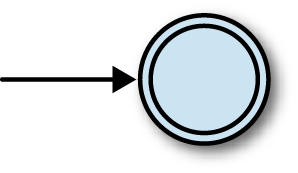
Here’s a way of visualizing the structure of one particular finite automaton:
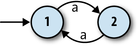
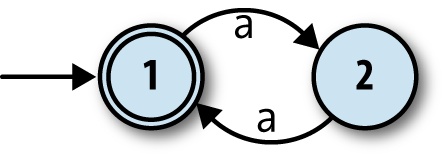
The two circles represent the automaton’s two states, 1 and 2, and the arrow coming from nowhere shows that the automaton always starts in state 1, its start state. The arrows between states represent the rules of the machine, which are:
When in state 1 and the character
ais read, move into state 2.When in state 2 and the character
ais read, move into state 1.
This is enough information for us to investigate how the machine processes a stream of inputs:
The machine starts in state 1.
The machine only has rules for reading the character
afrom its input stream, so that’s the only thing that can happen. When it reads ana, it moves from state 1 into state 2.When the machine reads another
a, it moves back into state 1.
Once it gets back to state 1, it’ll start repeating itself, so that’s the extent of this particular machine’s behavior. Information about the current state is assumed to be internal to the automaton—it operates as a “black box” that doesn’t reveal its inner workings—so the boringness of this behavior is compounded by the uselessness of it not causing any kind of observable output. Nobody in the outside world can see that anything is happening while the machine is bouncing between states 1 and 2, so in this case, we might as well have a single state and not bother with any internal structure at all.
Output
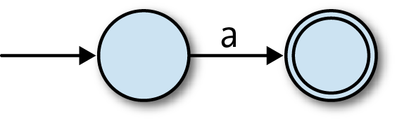
To address this problem, finite automata also have a rudimentary way of producing output. This is nothing as sophisticated as the output capabilities of real computers; we just mark some of the states as being special, and say that the machine’s single-bit output is the information about whether it’s currently in a special state or not. For this machine, let’s make state 2 a special state and show it on the diagram with a double circle:
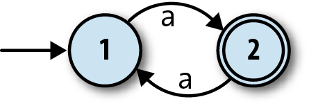
These special states are usually called
accept states, which suggests the idea of a machine
accepting or rejecting certain sequences of
inputs. If this automaton starts in state 1 and reads a single a, it will be left in state 2, which is an accept state, so we can say that the
machine accepts the string 'a'. On the other hand, if it
first reads an a and then another a, it’ll end up back in state 1, which isn’t an accept state, so
the machine rejects the string 'aa'. In fact, it’s easy
to see that this machine accepts any string of as whose
length is an odd number: 'a', 'aaa', 'aaaaa' are all accepted, while
'aa', 'aaaa', and
'' (the empty string) are rejected.
Now we have something slightly more useful: a machine that can read a sequence of characters and provide a yes/no output to indicate whether that sequence has been accepted. It’s reasonable to say that this DFA is performing a computation, because we can ask it a question—“is the length of this string an odd number?”—and get a meaningful reply back. This is arguably enough to call it a simple computer, and we can see how its features stack up against a real computer:
| Real computer | Finite automaton | |
| Permanent storage | Hard drive or SSD | None |
| Temporary storage | RAM | Current state |
| Input | Keyboard, mouse, network, etc. | Character stream |
| Output | Display device, speakers, network, etc. | Whether current state is an accept state (yes/no) |
| Processor | CPU core(s) that can execute any program | Hardcoded rules for changing state in response to input |
Of course, this specific automaton doesn’t do anything
sophisticated or useful, but we can build more complex automata that
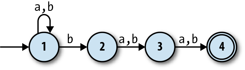
have more states and can read more than one character. Here’s one with
three states and the ability to read the inputs a and b:
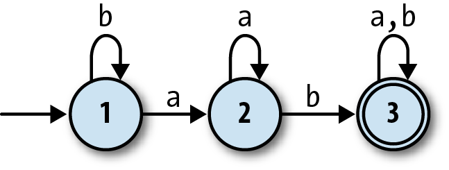
This machine accepts strings like 'ab', 'baba', and 'aaaab', and
rejects strings like 'a', 'baa', and 'bbbba'. A bit of experimentation
shows that it will only accept strings that contain the sequence 'ab', which still isn’t hugely useful but at least demonstrates a degree of
subtlety. We’ll see more practical applications later in the chapter.
Determinism
Significantly, this kind of automaton is deterministic: whatever state it’s currently in, and whichever character it reads, it’s always absolutely certain which state it will end up in. This certainty is guaranteed as long as we respect two constraints:
No contradictions: there are no states where the machine’s next move is ambiguous because of conflicting rules. (This implies that no state may have more than one rule for the same input character.)
No omissions: there are no states where the machine’s next move is unknown because of a missing rule. (This implies that every state must have at least one rule for each possible input character.)
Taken together, these constraints mean that the machine must have exactly one rule for each combination of state and input. The technical name for a machine that obeys the determinism constraints is a deterministic finite automaton (DFA).
Simulation
Deterministic finite automata are intended as abstract models of computation. We’ve drawn diagrams of a couple of example machines and thought about their behavior, but these machines don’t physically exist, so we can’t literally feed them input and see how they behave. Fortunately DFAs are so simple that we can easily build a simulation of one in Ruby and interact with it directly.
Let’s begin building that simulation by implementing a collection of rules, which we’ll call a rulebook:
classFARule<Struct.new(:state,:character,:next_state)defapplies_to?(state,character)self.state==state&&self.character==characterenddeffollownext_stateenddefinspect"#<FARule#{state.inspect}--#{character}-->#{next_state.inspect}>"endendclassDFARulebook<Struct.new(:rules)defnext_state(state,character)rule_for(state,character).followenddefrule_for(state,character)rules.detect{|rule|rule.applies_to?(state,character)}endend
This code establishes a simple API for rules: each rule has an
#applies_to? method, which returns
true or false to indicate whether that rule applies in
a particular situation, and a #follow
method that returns information about how the machine should change when
a rule is followed.[20] DFARulebook#next_state
uses these methods to locate the correct rule and discover what the next state of
the DFA should be.
Note
By using Enumerable#detect,
the implementation of DFARulebook#next_state assumes that there
will always be exactly one rule that applies to the given state and
character. If there’s more than one applicable rule, only the first
will have any effect and the others will be ignored; if there are
none, the #detect call will return
nil and the simulation will crash
when it tries to call nil.follow.
This is why the class is called DFARulebook rather than just FARulebook: it only works properly if the
determinism constraints are respected.
A rulebook lets us wrap up many rules into a single object and ask it questions about which state comes next:
>>rulebook=DFARulebook.new([FARule.new(1,'a',2),FARule.new(1,'b',1),FARule.new(2,'a',2),FARule.new(2,'b',3),FARule.new(3,'a',3),FARule.new(3,'b',3)])=> #<struct DFARulebook …>>>rulebook.next_state(1,'a')=> 2>>rulebook.next_state(1,'b')=> 1>>rulebook.next_state(2,'b')=> 3
Note
We had a choice here about how to represent the states of our automaton as Ruby
values. All that matters is the ability to tell the states apart: our implementation of
DFARulebook#next_state needs to be able to compare
two states to decide whether they’re the same, but otherwise, it doesn’t care whether
those objects are numbers, symbols, strings, hashes, or faceless instances of the Object class.
In this case, it’s clearest to use plain old Ruby numbers—they match up nicely with the numbered states on the diagrams—so we’ll do that for now.
Once we have a rulebook, we can use it to build a DFA object that keeps track of its current
state and can report whether it’s currently in an accept state or
not:
classDFA<Struct.new(:current_state,:accept_states,:rulebook)defaccepting?accept_states.include?(current_state)endend
>>DFA.new(1,[1,3],rulebook).accepting?=> true>>DFA.new(1,[3],rulebook).accepting?=> false
We can now write a method to read a character of input, consult the rulebook, and change state accordingly:
classDFAdefread_character(character)self.current_state=rulebook.next_state(current_state,character)endend
This lets us feed characters to the DFA and watch its output change:
>>dfa=DFA.new(1,[3],rulebook);dfa.accepting?=> false>>dfa.read_character('b');dfa.accepting?=> false>>3.timesdodfa.read_character('a')end;dfa.accepting?=> false>>dfa.read_character('b');dfa.accepting?=> true
Feeding the DFA one character at a time is a little unwieldy, so let’s add a convenience method for reading an entire string of input:
classDFAdefread_string(string)string.chars.eachdo|character|read_character(character)endendend
Now we can provide the DFA a whole string of input instead of having to pass its characters individually:
>>dfa=DFA.new(1,[3],rulebook);dfa.accepting?=> false>>dfa.read_string('baaab');dfa.accepting?=> true
Once a DFA object has been fed some input, it’s probably not in its start state anymore, so we can’t reliably reuse it to check a completely new sequence of inputs. That means we have to recreate it from scratch—using the same start state, accept states, and rulebook as before—every time we want to see whether it will accept a new string. We can avoid doing this manually by wrapping up its constructor’s arguments in an object that represents the design of a particular DFA and relying on that object to automatically build one-off instances of that DFA whenever we want to check for acceptance of a string:
classDFADesign<Struct.new(:start_state,:accept_states,:rulebook)defto_dfaDFA.new(start_state,accept_states,rulebook)enddefaccepts?(string)to_dfa.tap{|dfa|dfa.read_string(string)}.accepting?endend
Note
The #tap method evaluates a
block and then returns the object it was called on.
DFADesign#accepts? uses the
DFADesign#to_dfa method to create a
new instance of DFA and then calls
#read_string? to put it into an accepting or rejecting state:
>>dfa_design=DFADesign.new(1,[3],rulebook)=> #<struct DFADesign …>>>dfa_design.accepts?('a')=> false>>dfa_design.accepts?('baa')=> false>>dfa_design.accepts?('baba')=> true
Nondeterministic Finite Automata
DFAs are simple to understand and to implement, but that’s because they’re very similar to machines we’re already familiar with. Having stripped away all the complexity of a real computer, we now have the opportunity to experiment with less conventional ideas that take us further away from the machines we’re used to, without having to deal with the incidental difficulties of making those ideas work in a real system.
One way to explore is by chipping away at our existing assumptions and constraints. For one thing, the determinism constraints seem restrictive: maybe we don’t care about every possible input character at every state, so why can’t we just leave out rules for characters we don’t care about and assume that the machine can go into a generic failure state when something unexpected happens? More exotically, what would it mean to allow the machine to have contradictory rules, so that more than one execution path is possible? Our setup also assumes that each state change must happen in response to a character being read from the input stream, but what would happen if the machine could change state without having to read anything?
In this section, we’ll investigate these ideas and see what new possibilities are opened up by tweaking a finite automaton’s capabilities.
Nondeterminism
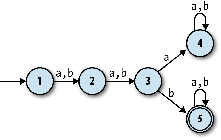
Suppose we wanted a finite automaton that would accept any string of
as and bs as long as the third character was b. It’s easy enough to come up with a suitable
DFA design:
What if we wanted a machine that would accept strings where the
third-from-last character is b? How would that work? It seems more
difficult: the DFA above is guaranteed to be in state 3 when it reads
the third character, but a machine can’t know in advance
when it’s reading the third-from-last character,
because it doesn’t know how long the string is until it’s finished
reading it. It might not be immediately clear whether such a DFA is even
possible.
However, if we relax the determinism constraints and allow the rulebook to contain multiple rules (or no rules at all) for a given state and input, we can design a machine that does the job:
This state machine, a nondeterministic finite
automaton (NFA), no longer has exactly one execution path
for each sequence of inputs. When it’s in state 1 and reads b as input, it’s possible for it to follow a
rule that keeps it in state 1, but it’s also possible for it to follow a
different rule that takes it into state 2 instead. Conversely, once it
gets into state 4, it has no rules to follow and therefore no way to
read any more input. A DFA’s next state is always completely determined
by its current state and its input, but an NFA sometimes has more than
one possibility for which state to move into next, and sometimes none at
all.
A DFA accepts a string if reading the characters and blindly following the rules causes the machine to end up in an accept state, so what does it mean for an NFA to accept or reject a string? The natural answer is that a string is accepted if there’s some way for the NFA to end up in an accept state by following some of its rules—that is, if finishing in an accept state is possible, even if it’s not inevitable.
For example, this NFA accepts the string 'baa',
because, starting at state 1, the rules say there is a way for the machine to read a
b and move into state 2, then read an a and move into state 3, and finally read another a and finish in state 4, which is an accept state. It also
accepts the string 'bbbbb', because it’s possible for the
NFA to initially follow a different rule and stay in state 1 while reading the first two
bs, and only use the rule for moving into state 2 when
reading the third b, which then lets it read the rest of
the string and finish in state 4 as before.
On the other hand, there’s no way for it to read 'abb' and end up in state 4—depending on which rules it follows, it can only
end up in state 1, 2, or 3—so 'abb' is not accepted by
this NFA. Neither is 'bbabb', which can only ever get as
far as state 3; if it goes straight into state 2 when reading the first b, it will end up in state 4 too early, with two characters
still left to read but no more rules to follow.
Note
The collection of strings that are accepted by a particular machine is called a language: we say that the machine recognizes that language. Not all possible languages have a DFA or NFA that can recognize them (see Chapter 4 for more information), but those languages that can be recognized by finite automata are called regular languages.
Relaxing the determinism constraints has produced an imaginary machine that is very different from the real, deterministic computers we’re familiar with. An NFA deals in possibilities rather than certainties; we talk about its behavior in terms of what can happen rather than what will happen. This seems powerful, but how can such a machine work in the real world? At first glance it looks like a real implementation of an NFA would need some kind of foresight in order to know which of several possibilities to choose while it reads input: to stand a chance of accepting a string, our example NFA must stay in state 1 until it reads the third-from-last character, but it has no way of knowing how many more characters it will receive. How can we simulate an exciting machine like this in boring, deterministic Ruby?
The key to simulating an NFA on a deterministic computer is to find a way to explore all possible executions of the machine. This brute-force approach eliminates the spooky foresight that would be required to simulate only one possible execution by somehow making all the right decisions along the way. When an NFA reads a character, there are only ever a finite number of possibilities for what it can do next, so we can simulate the nondeterminism by somehow trying all of them and seeing whether any of them ultimately allows it to reach an accept state.
We could do this by recursively trying all possibilities: each time the simulated NFA reads a character and there’s more than one applicable rule, follow one of those rules and try reading the rest of the input; if that doesn’t leave the machine in an accept state, then go back into the earlier state, rewind the input to its earlier position, and try again by following a different rule; repeat until some choice of rules leads to an accept state, or until all possible choices have been tried without success.
Another strategy is to simulate all possibilities in parallel by spawning new threads every time the machine has more than one rule it can follow next, effectively copying the simulated NFA so that each copy can try a different rule to see how it pans out. All those threads can be run at once, each reading from its own copy of the input string, and if any thread ends up with a machine that’s read every character and stopped in an accept state, then we can say the string has been accepted.
Both of these implementations are feasible, but they’re a bit complicated and inefficient. Our DFA simulation was simple and could read individual characters while constantly reporting back on whether the machine is in an accept state, so it would be nice to simulate an NFA in a way that gives us the same simplicity and transparency.
Fortunately, there’s an easy way to simulate an NFA without needing to rewind our progress, spawn threads, or know all the input characters in advance. In fact, just as we simulated a single DFA by keeping track of its current state, we can simulate a single NFA by keeping track of all its possible current states. This is simpler and more efficient than simulating multiple NFAs that go off in different directions, and it turns out to achieve the same thing in the end. If we did simulate many separate machines, then all we’d care about is what state each of them was in, but any machines in the same state are completely indistinguishable,[21] so we don’t lose anything by collapsing all those possibilities down into a single machine and asking “which states could it be in by now?” instead.
For example, let’s walk through what happens to our example NFA as it reads the string
'bab':
Before the NFA has read any input, it’s definitely in state 1, its start state.
It reads the first character,
b. From state 1, there’s onebrule that lets the NFA stay in state 1 and anotherbrule that takes it to state 2, so we know it can be in either state 1 or 2 afterward. Neither of those is an accept state, which tells us there’s no possible way for the NFA to reach an accept state by reading the string'b'.It reads the second character,
a. If it’s in state 1 then there’s only onearule it can follow, which will keep it in state 1; if it’s in state 2, it’ll have to follow thearule that leads to state 3. It must end up in state 1 or 3, and again, these aren’t accept states, so there’s no way the string'ba'can be accepted by this machine.It reads the third character,
b. If it’s in state 1 then, as before it can stay in state 1 or go to state 2; if it’s in state 3, then it must go to state 4.Now we know that it’s possible for the NFA to be in state 1, state 2, or state 4 after reading the whole input string. State 4 is an accept state, and our simulation shows that there must be some way for the machine to reach state 4 by reading that string, so the NFA does accept
'bab'.
This simulation strategy is easy to turn into code. First we need a rulebook suitable for storing an NFA’s rules. A DFA rulebook always returns a single state when we ask it where the DFA should go next after reading a particular character while in a specific state, but an NFA rulebook needs to answer a different question: when an NFA is possibly in one of several states, and it reads a particular character, what states can it possibly be in next? The implementation looks like this:
require'set'classNFARulebook<Struct.new(:rules)defnext_states(states,character)states.flat_map{|state|follow_rules_for(state,character)}.to_setenddeffollow_rules_for(state,character)rules_for(state,character).map(&:follow)enddefrules_for(state,character)rules.select{|rule|rule.applies_to?(state,character)}endend
Note
We’re using the Set class,
from Ruby’s standard library, to store the collection of possible
states returned by #next_states. We
could have used an Array, but
Set has three useful
features:
It automatically eliminates duplicate elements.
Set[1, 2, 2, 3, 3, 3]is equal toSet[1, 2, 3].It ignores the order of elements.
Set[3, 2, 1]is equal toSet[1, 2, 3].It provides standard set operations like intersection (
#&), union (#+), and subset testing (#subset?).
The first feature is useful because it doesn’t make sense to say
“the NFA is in state 3 or state 3,” and returning a Set makes sure we never include any
duplicates. The other two features will be useful later.
We can create a nondeterministic rulebook and ask it questions:
>>rulebook=NFARulebook.new([FARule.new(1,'a',1),FARule.new(1,'b',1),FARule.new(1,'b',2),FARule.new(2,'a',3),FARule.new(2,'b',3),FARule.new(3,'a',4),FARule.new(3,'b',4)])=> #<struct NFARulebook rules=[…]>>>rulebook.next_states(Set[1],'b')=> #<Set: {1, 2}>>>rulebook.next_states(Set[1,2],'a')=> #<Set: {1, 3}>>>rulebook.next_states(Set[1,3],'b')=> #<Set: {1, 2, 4}>
The next step is to implement an NFA class to represent the simulated
machine:
classNFA<Struct.new(:current_states,:accept_states,:rulebook)defaccepting?(current_states&accept_states).any?endend
Note
NFA#accepting? works by
checking whether there are any states in the intersection between
current_states and accept_states—that is, whether any of the
possible current states is also one of the accept states.
This NFA class is very similar
to our DFA class from earlier. The
difference is that it has a set of possible current_states instead of a single definite
current_state, so it’ll say it’s in
an accept state if any of its current_states is an accept state:
>>NFA.new(Set[1],[4],rulebook).accepting?=> false>>NFA.new(Set[1,2,4],[4],rulebook).accepting?=> true
As with the DFA class, we can
implement a #read_character method
for reading a single character of input, and a #read_string method for reading several in
sequence:
classNFAdefread_character(character)self.current_states=rulebook.next_states(current_states,character)enddefread_string(string)string.chars.eachdo|character|read_character(character)endendend
These methods really are almost identical to their DFA counterparts; we’re just saying current_states and next_states in #read_character instead of current_state and next_state.
That’s the hard work over with. Now we’re able to start a simulated NFA, pass characters in, and ask whether the input so far has been accepted:
>>nfa=NFA.new(Set[1],[4],rulebook);nfa.accepting?=> false>>nfa.read_character('b');nfa.accepting?=> false>>nfa.read_character('a');nfa.accepting?=> false>>nfa.read_character('b');nfa.accepting?=> true>>nfa=NFA.new(Set[1],[4],rulebook)=> #<struct NFA current_states=#<Set: {1}>, accept_states=[4], rulebook=…>>>nfa.accepting?=> false>>nfa.read_string('bbbbb');nfa.accepting?=> true
As we saw with the DFA class,
it’s convenient to use an NFADesign
object to automatically manufacture new NFA instances on demand rather than creating
them manually:
classNFADesign<Struct.new(:start_state,:accept_states,:rulebook)defaccepts?(string)to_nfa.tap{|nfa|nfa.read_string(string)}.accepting?enddefto_nfaNFA.new(Set[start_state],accept_states,rulebook)endend
This makes it easier to check different strings against the same NFA:
>>nfa_design=NFADesign.new(1,[4],rulebook)=> #<struct NFADesign start_state=1, accept_states=[4], rulebook=…>>>nfa_design.accepts?('bab')=> true>>nfa_design.accepts?('bbbbb')=> true>>nfa_design.accepts?('bbabb')=> false
And that’s it: we’ve successfully built a simple implementation of an unusual nondeterministic machine by simulating all of its possible executions. Nondeterminism is a convenient tool for designing more sophisticated finite automata, so it’s fortunate that NFAs are usable in practice rather than just a theoretical curiosity.
Free Moves
We’ve seen how relaxing the determinism constraints gives us new ways of designing machines without sacrificing our ability to implement them. What else can we safely relax to give ourselves more design freedom?
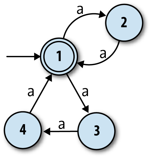
It’s easy to design a DFA that accepts strings of as
whose length is a multiple of two ('aa', 'aaaa'…):
But how can we design a machine that accepts strings whose length is a multiple of two or three? We know that nondeterminism gives a machine more than one execution path to follow, so perhaps we can design an NFA that has one “multiple of two” path and one “multiple of three” path. A naïve attempt might look like this:
The idea here is for the NFA to move between states 1 and 2 to accept strings like
'aa' and 'aaaa', and
between states 1, 3, and 4 to accept strings like 'aaa'
and 'aaaaaaaaa'. That works fine, but the problem is that
the machine also accepts the string 'aaaaa', because it
can move from state 1 to state 2 and back to 1 when reading the first two characters, and
then move through states 3, 4, and back to 1 when reading the next three, ending up in an
accept state even though the string’s length is not a multiple of two or three.[22]
Again it may not be immediately obvious whether an NFA can do this job at all, but we can address the problem by introducing another machine feature called free moves. These are rules that the machine may spontaneously follow without reading any input, and they help here because they give the NFA an initial choice between two separate groups of states:
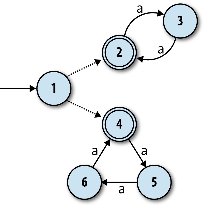
The free moves are shown by the dotted unlabeled arrows from state 1 to states 2 and 4.
This machine can still accept the string 'aaaa' by
spontaneously moving into state 2, and then moving between states 2 and 3 as it reads the
input, and likewise for 'aaaaaaaaa' if it begins with a
free move into state 4. Now, though, there is no way for it to accept the string 'aaaaa': in any possible execution, it must begin by committing
to a free move into either state 2 or state 4, and once it’s gone one way, there’s no route
back again. Once it’s in state 2, it can only accept a string whose length is a multiple of
2, and likewise once it’s in state 4, it can only accept a string whose length is a multiple
of 3.
How do we support free moves in our Ruby NFA simulation? Well, this new choice between staying in state 1, spontaneously moving into state 2, or spontaneously moving into state 4 is not really any stranger than the nondeterminism we already have, and our implementation can handle it in a similar way. We already have the idea of a simulated machine having many possible states at once, so we just need to broaden those possible states to include any that are reachable by performing one or more free moves. In this case, the machine starting in state 1 really means that it can be in state 1, 2, or 4 before it’s read any input.
First we need a way to represent free moves in Ruby. The easiest
way is to use normal FARule instances
with a nil where a character should
be. Our existing implementation of NFARulebook will treat nil like any other character, so we can ask
“from state 1, what states can we get to by performing one free move?”
(instead of “…by reading one a
character?”):
>>rulebook=NFARulebook.new([FARule.new(1,nil,2),FARule.new(1,nil,4),FARule.new(2,'a',3),FARule.new(3,'a',2),FARule.new(4,'a',5),FARule.new(5,'a',6),FARule.new(6,'a',4)])=> #<struct NFARulebook rules=[…]>>>rulebook.next_states(Set[1],nil)=> #<Set: {2, 4}>
Next we need some helper code for finding all the states that can be reached by
following free moves from a particular set of states. This code will have to follow free
moves repeatedly, because an NFA can spontaneously change states as many times as it likes
as long as there are free moves leading from its current state. A method on the NFARulebook class is a convenient place to put it:
classNFARulebookdeffollow_free_moves(states)more_states=next_states(states,nil)ifmore_states.subset?(states)stateselsefollow_free_moves(states+more_states)endendend
NFARulebook#follow_free_moves works by recursively
looking for more and more states that can be reached from a given set of states by following
free moves. When it can’t find any more—that is, when every state found by next_states(states, nil) is already in states—it returns all the states it’s found.[23]
This code correctly identifies the possible states of our NFA before it’s read any input:
>>rulebook.follow_free_moves(Set[1])=> #<Set: {1, 2, 4}>
Now we can bake this free move support into NFA by overriding the existing implementation
of NFA#current_states (as provided by
Struct). Our new implementation will
hook into NFARulebook#follow_free_moves and ensure that
the possible current states of the automaton always include any states
that are reachable via free moves:
classNFAdefcurrent_statesrulebook.follow_free_moves(super)endend
Since all other NFA methods
access the set of possible current states by calling the #current_states method, this transparently
provides support for free moves without having to change the rest of
NFA’s code.
That’s it. Now our simulation supports free moves, and we can see which strings are accepted by our NFA:
>>nfa_design=NFADesign.new(1,[2,4],rulebook)=> #<struct NFADesign …>>>nfa_design.accepts?('aa')=> true>>nfa_design.accepts?('aaa')=> true>>nfa_design.accepts?('aaaaa')=> false>>nfa_design.accepts?('aaaaaa')=> true
So free moves are pretty straightforward to implement, and they give us extra design freedom on top of what nondeterminism already provides.
Note
Some of the terminology in this chapter is unconventional. The characters read by finite automata are usually called symbols, the rules for moving between states are called transitions, and the collection of rules making up a machine is called a transition function (or sometimes transition relation for NFAs) rather than a rulebook. Because the mathematical symbol for the empty string is the Greek letter ε (epsilon), an NFA with free moves is known as an NFA-ε, and free moves themselves are usually called ε-transitions.
Regular Expressions
We’ve seen that nondeterminism and free moves make finite automata more expressive without interfering with our ability to simulate them. In this section, we’ll look at an important practical application of these features: regular expression matching.
Regular expressions provide a language for writing textual patterns against which strings may be matched. Some example regular expressions are:
hello, which only matches the string'hello'hello|goodbye, which matches the strings'hello'and'goodbye'(hello)*, which matches the strings'hello','hellohello','hellohellohello', and so on, as well as the empty string
Warning
In this chapter, we’ll always think of a regular expression as matching an entire string. Real-world implementations of regular expressions typically use them for matching parts of strings, with extra syntax needed if we want to specify that an entire string should be matched.
For example, our regular expression hello|goodbye would be written in Ruby as
/A(hello|goodbye)z/ to make sure
that any match is anchored to the beginning (A) and end (z) of the string.
Given a regular expression and a string, how do we write a program to decide whether the string matches that expression? Most programming languages, Ruby included, already have regular expression support built in, but how does that support work? How would we implement regular expressions in Ruby if the language didn’t already have them?
It turns out that finite automata are perfectly suited to this job. As we’ll see, it’s possible to convert any regular expression into an equivalent NFA—every string matched by the regular expression is accepted by the NFA, and vice versa—and then match a string by feeding it to a simulation of that NFA to see whether it gets accepted. In the language of Chapter 2, we can think of this as providing a sort of denotational semantics for regular expressions: we may not know how to execute a regular expression directly, but we can show how to denote it as an NFA, and because we have an operational semantics for NFAs (“change state by reading characters and following rules”), we can execute the denotation to achieve the same result.
Syntax
Let’s be precise about what we mean by “regular expression.” To get us off the ground, here are two kinds of extremely simple regular expression that are not built out of anything simpler:
An empty regular expression. This matches the empty string and nothing else.
A regular expression containing a single, literal character. For example,
aandbare regular expressions that match only the strings'a'and'b'respectively.
Once we have these simple kinds of pattern, there are three ways we can combine them to build more complex expressions:
Concatenate two patterns. We can concatenate the regular expressions
aandbto get the regular expressionab, which only matches the string'ab'.Choose between two patterns, written by joining them with the
|operator. We can join the regular expressionsaorbto get the regular expressiona|b, which matches the strings'a'and'b'.Repeat a pattern zero or more times, written by suffixing it with the
*operator. We can suffix the regular expressionato geta*, which matches the strings'a','aa','aaa', and so on, as well as the empty string''(i.e., zero repetitions).
Note
Real-world regular expression engines, like the one built into Ruby, support more features than this. In the interests of simplicity, we won’t try to implement these extra features, many of which are technically redundant and only provided as a convenience.
For example, omitting the repetition operators ?
and + doesn’t make an important difference, because
their effects—“repeat one or zero times” and “repeat one or more times,” respectively—are
easy enough to achieve with the features we already have: the regular expression ab? can be rewritten as ab|a, and the pattern ab+ matches the same
strings as abb*. The same is true of other convenience
features like counted repetition (e.g., a{2,5}) and
character classes (e.g., [abc]).
More advanced features like capture groups, backreferences and lookahead/lookbehind assertions are outside of the scope of this chapter.
To implement this syntax in Ruby, we can define a class for each kind of regular expression and use instances of those classes to represent the abstract syntax tree of any regular expression, just as we did for Simple expressions in Chapter 2:
modulePatterndefbracket(outer_precedence)ifprecedence<outer_precedence'('+to_s+')'elseto_sendenddefinspect"/#{self}/"endendclassEmptyincludePatterndefto_s''enddefprecedence3endendclassLiteral<Struct.new(:character)includePatterndefto_scharacterenddefprecedence3endendclassConcatenate<Struct.new(:first,:second)includePatterndefto_s[first,second].map{|pattern|pattern.bracket(precedence)}.joinenddefprecedence1endendclassChoose<Struct.new(:first,:second)includePatterndefto_s[first,second].map{|pattern|pattern.bracket(precedence)}.join('|')enddefprecedence0endendclassRepeat<Struct.new(:pattern)includePatterndefto_spattern.bracket(precedence)+'*'enddefprecedence2endend
Note
In the same way that multiplication binds its arguments more tightly than addition in
arithmetic expressions (1 + 2 × 3 equals 7, not 9), the convention for the concrete syntax
of regular expressions is for the * operator to bind
more tightly than concatenation, which in turn binds more tightly than the | operator. For example, in the regular expression abc* it’s understood that the * applies only to the c ('abc', 'abcc', 'abccc'…), and to make it apply to all of abc ('abc', 'abcabc'…), we’d need to add brackets and write (abc)* instead.
The syntax classes’ implementations of #to_s, along with the Pattern#bracket method, deal with
automatically inserting these brackets when necessary so that we can
view a simple string representation of an abstract syntax tree without
losing information about its structure.
These classes let us manually build trees to represent regular expressions:
>>pattern=Repeat.new(Choose.new(Concatenate.new(Literal.new('a'),Literal.new('b')),Literal.new('a')))=> /(ab|a)*/
Of course, in a real implementation, we’d use a parser to build these trees instead of constructing them by hand; see Parsing for instructions on how to do this.
Semantics
Now that we have a way of representing the syntax of a regular expression as a tree of Ruby objects, how can we convert that syntax into an NFA?
We need to decide how instances of each syntax class should be
turned into NFAs. The easiest class to convert is Empty, which we should always turn into the
one-state NFA that only accepts the empty string:
Similarly, we should turn any literal, single-character pattern
into the NFA that only accepts the single-character string containing
that character. Here’s the NFA for the pattern a:
It’s easy enough to implement #to_nfa_design methods for Empty and Literal to generate these NFAs:
classEmptydefto_nfa_designstart_state=Object.newaccept_states=[start_state]rulebook=NFARulebook.new([])NFADesign.new(start_state,accept_states,rulebook)endendclassLiteraldefto_nfa_designstart_state=Object.newaccept_state=Object.newrule=FARule.new(start_state,character,accept_state)rulebook=NFARulebook.new([rule])NFADesign.new(start_state,[accept_state],rulebook)endend
Note
As mentioned in Simulation, the states of an automaton must be
implemented as Ruby objects that can be distinguished from each other. Here, instead of
using numbers (i.e., Fixnum instances) as states, we’re
using freshly created instances of Object.
This is so that each NFA gets its own unique states, which gives
us the ability to combine small machines into larger ones without
accidentally merging any of their states. If two distinct NFAs both
used the Ruby Fixnum object
1 as a state, for example, they
couldn’t be connected together while keeping those two states
separate. We’ll want to be able to do that as part of implementing
more complex regular expressions.
Similarly, we won’t label states on the diagrams any more, so that we don’t have to relabel them when we start connecting diagrams together.
We can check that the NFAs generated from Empty and Literal regular expressions accept the strings
we want them to:
>>nfa_design=Empty.new.to_nfa_design=> #<struct NFADesign …>>>nfa_design.accepts?('')=> true>>nfa_design.accepts?('a')=> false>>nfa_design=Literal.new('a').to_nfa_design=> #<struct NFADesign …>>>nfa_design.accepts?('')=> false>>nfa_design.accepts?('a')=> true>>nfa_design.accepts?('b')=> false
There’s an opportunity here to wrap #to_nfa_design in a #matches? method to give patterns a nicer
interface:
modulePatterndefmatches?(string)to_nfa_design.accepts?(string)endend
This lets us match patterns directly against strings:
>>Empty.new.matches?('a')=> false>>Literal.new('a').matches?('a')=> true
Now that we know how to turn simple Empty and Literal regular expressions into NFAs, we need
a similar setup for Concatenate,
Choose, and Repeat.
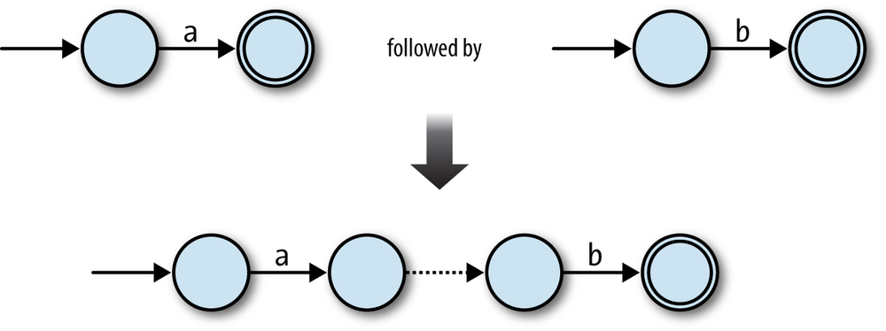
Let’s begin with Concatenate:
if we have two regular expressions that we already know how to turn into
NFAs, how can we build an NFA to represent the concatenation of those
regular expressions? For example, given that we can turn
the single-character regular expressions a and b
into NFAs, how do we turn ab into
one?
In the ab case, we can connect the two NFAs in
sequence, joining them together with a free move, and keeping the second NFA’s accept
state:
This technique works in other cases too. Any two NFAs can be concatenated by turning every accept state from the first NFA into a nonaccept state and connecting it to the start state of the second NFA with a free move. Once the concatenated machine has read a sequence of inputs that would have put the first NFA into an accept state, it can spontaneously move into a state corresponding to the start state of the second NFA, and then reach an accept state by reading a sequence of inputs that the second NFA would have accepted.
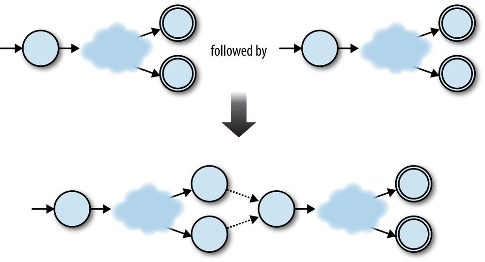
So, the raw ingredients for the combined machine are:
The start state of the first NFA
The accept states of the second NFA
All the rules from both NFAs
Some extra free moves to connect each of the first NFA’s old accept states to the second NFA’s old start state
We can turn this idea into an implementation of Concatenate#to_nfa_design:
classConcatenatedefto_nfa_designfirst_nfa_design=first.to_nfa_designsecond_nfa_design=second.to_nfa_designstart_state=first_nfa_design.start_stateaccept_states=second_nfa_design.accept_statesrules=first_nfa_design.rulebook.rules+second_nfa_design.rulebook.rulesextra_rules=first_nfa_design.accept_states.map{|state|FARule.new(state,nil,second_nfa_design.start_state)}rulebook=NFARulebook.new(rules+extra_rules)NFADesign.new(start_state,accept_states,rulebook)endend
This code first converts the first and second regular expressions
into NFADesigns, then combines their
states and rules in the appropriate way to make a new NFADesign. It works as expected for the simple
ab case:
>>pattern=Concatenate.new(Literal.new('a'),Literal.new('b'))=> /ab/>>pattern.matches?('a')=> false>>pattern.matches?('ab')=> true>>pattern.matches?('abc')=> false
This conversion process is recursive—Concatenate#to_nfa_design calls #to_nfa_design on other objects—so it also
works for more deeply nested cases like the regular expression abc, which contains two concatenations
(a concatenated with b concatenated with c):
>>pattern=Concatenate.new(Literal.new('a'),Concatenate.new(Literal.new('b'),Literal.new('c')))=> /abc/>>pattern.matches?('a')=> false>>pattern.matches?('ab')=> false>>pattern.matches?('abc')=> true
Note
This is another example of a denotational semantics being compositional: the NFA denotation of a compound regular expression is composed from the denotations of its parts.
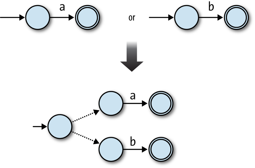
We can use a similar strategy to convert a Choose expression into an NFA. In the simplest
case, the NFAs for the regular expressions a and b can
be combined to build an NFA for the regular expression a|b by adding a new start state and using free
moves to connect it to the previous start states of the two original
machines:
Before the a|b NFA has read any input, it can use a
free move to go into either of the original machines’ start states, from which point it can
read either 'a' or 'b'
to reach an accept state. Again, it’s just as easy to glue together any two machines by
adding a new start state and two free moves:
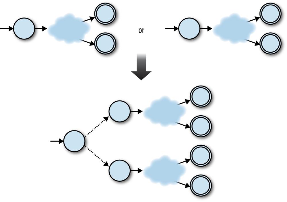
In this case, the ingredients for the combined machine are:
A new start state
All the accept states from both NFAs
All the rules from both NFAs
Two extra free moves to connect the new start state to each of the NFA’s old start states
Again, this is easy to implement as Choose#to_nfa_design:
classChoosedefto_nfa_designfirst_nfa_design=first.to_nfa_designsecond_nfa_design=second.to_nfa_designstart_state=Object.newaccept_states=first_nfa_design.accept_states+second_nfa_design.accept_statesrules=first_nfa_design.rulebook.rules+second_nfa_design.rulebook.rulesextra_rules=[first_nfa_design,second_nfa_design].map{|nfa_design|FARule.new(start_state,nil,nfa_design.start_state)}rulebook=NFARulebook.new(rules+extra_rules)NFADesign.new(start_state,accept_states,rulebook)endend
The implementation works nicely:
>>pattern=Choose.new(Literal.new('a'),Literal.new('b'))=> /a|b/>>pattern.matches?('a')=> true>>pattern.matches?('b')=> true>>pattern.matches?('c')=> false
And finally, repetition: how can we turn an NFA that matches a
string exactly once into an NFA that matches the same string zero or
more times? We can build an NFA for a* by starting with the NFA for a and making two additions:
Add a free move from its accept state to its start state, so it can match more than one
'a'.Add a new accepting start state with a free move to the old start state, so it can match the empty string.
Here’s how that looks:
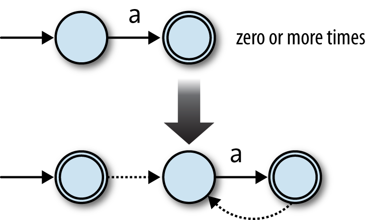
The free move from the old accept state to the old start state allows the machine to
match several times instead of just once ('aa', 'aaa', etc.), and the new start state allows it to match the
empty string without affecting what other strings it can accept.[24] We can do the same for any NFA as long as we connect each old accept state to
the old start state with a free move:
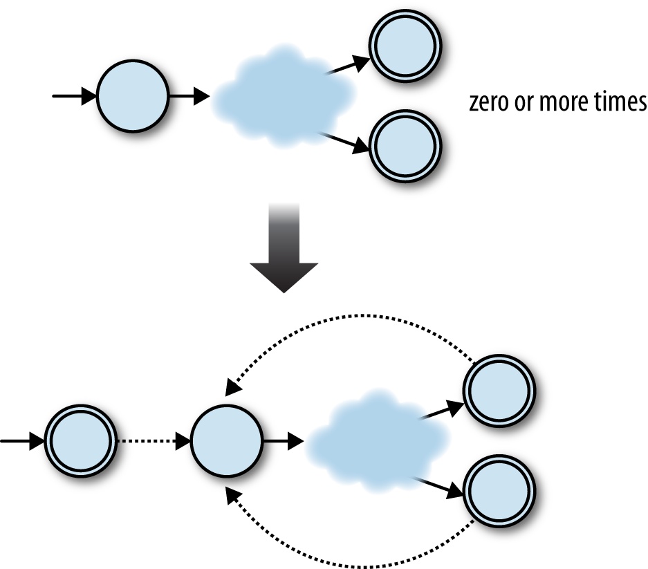
This time we need:
A new start state, which is also an accept state
All the accept states from the old NFA
All the rules from the old NFA
Some extra free moves to connect each of the old NFA’s accept states to its old start state
Another extra free move to connect the new start state to the old start state
Let’s turn that into code:
classRepeatdefto_nfa_designpattern_nfa_design=pattern.to_nfa_designstart_state=Object.newaccept_states=pattern_nfa_design.accept_states+[start_state]rules=pattern_nfa_design.rulebook.rulesextra_rules=pattern_nfa_design.accept_states.map{|accept_state|FARule.new(accept_state,nil,pattern_nfa_design.start_state)}+[FARule.new(start_state,nil,pattern_nfa_design.start_state)]rulebook=NFARulebook.new(rules+extra_rules)NFADesign.new(start_state,accept_states,rulebook)endend
And check that it works:
>>pattern=Repeat.new(Literal.new('a'))=> /a*/>>pattern.matches?('')=> true>>pattern.matches?('a')=> true>>pattern.matches?('aaaa')=> true>>pattern.matches?('b')=> false
Now that we have #to_nfa_design
implementations for each class of regular expression syntax, we can
build up complex patterns and use them to match strings:
>>pattern=Repeat.new(Concatenate.new(Literal.new('a'),Choose.new(Empty.new,Literal.new('b'))))=> /(a(|b))*/>>pattern.matches?('')=> true>>pattern.matches?('a')=> true>>pattern.matches?('ab')=> true>>pattern.matches?('aba')=> true>>pattern.matches?('abab')=> true>>pattern.matches?('abaab')=> true>>pattern.matches?('abba')=> false
This is a nice result. We began with a syntax for patterns and have now given a semantics for that syntax by showing how to convert any pattern into an NFA, a kind of abstract machine that we already know how to execute. In conjunction with a parser, this gives us a practical way of reading a regular expression and deciding whether it matches a particular string. Free moves are useful for this conversion because they provide an unobtrusive way to glue together smaller machines into larger ones without affecting the behavior of any of the components.
Note
The majority of real-world implementations of regular expressions, like the Onigmo library used by Ruby, don’t work by literally compiling patterns into finite automata and simulating their execution. Although it’s a fast and efficient way of matching regular expressions against strings, this approach makes it harder to support more advanced features like capture groups and lookahead/lookbehind assertions. Consequently most libraries use some kind of backtracking algorithm that deals with regular expressions more directly instead of converting them into finite automata.
Russ Cox’s RE2 library is a production-quality C++ regular expression implementation that does compile patterns into automata,[25] while Pat Shaughnessy has written a detailed blog post exploring how Ruby’s regular expression algorithm works.
Parsing
We’ve almost built a complete (albeit basic) regular expression implementation. The only
missing piece is a parser for pattern syntax: it would be much more convenient if we could
just write (a(|b))* instead of building the abstract
syntax tree manually with Repeat.new(Concatenate.new(Literal.new('a'), Choose.new(Empty.new,
Literal.new('b')))). We saw in Implementing Parsers that it’s
not difficult to use Treetop to generate a parser that can automatically transform raw
syntax into an AST, so let’s do that here to finish off our implementation.
Here’s a Treetop grammar for simple regular expressions:
grammarPatternrulechoosefirst:concatenate_or_empty'|'rest:choose{defto_astChoose.new(first.to_ast,rest.to_ast)end}/concatenate_or_emptyendruleconcatenate_or_emptyconcatenate/emptyendruleconcatenatefirst:repeatrest:concatenate{defto_astConcatenate.new(first.to_ast,rest.to_ast)end}/repeatendruleempty''{defto_astEmpty.newend}endrulerepeatbrackets'*'{defto_astRepeat.new(brackets.to_ast)end}/bracketsendrulebrackets'('choose')'{defto_astchoose.to_astend}/literalendruleliteral[a-z]{defto_astLiteral.new(text_value)end}endend
Note
Again, the order of rules reflects the precedence of each operator: the | operator binds loosest, so the choose rule goes first, with the higher precedence operator rules appearing
farther down the grammar.
Now we have all the pieces we need to parse a regular expression, turn it into an abstract syntax tree, and use it to match strings:
>>require'treetop'=> true>>Treetop.load('pattern')=> PatternParser>>parse_tree=PatternParser.new.parse('(a(|b))*')=> SyntaxNode+Repeat1+Repeat0 offset=0, "(a(|b))*" (to_ast,brackets):SyntaxNode+Brackets1+Brackets0 offset=0, "(a(|b))" (to_ast,choose):SyntaxNode offset=0, "("SyntaxNode+Concatenate1+Concatenate0 offset=1, "a(|b)" (to_ast,first,rest):SyntaxNode+Literal0 offset=1, "a" (to_ast)SyntaxNode+Brackets1+Brackets0 offset=2, "(|b)" (to_ast,choose):SyntaxNode offset=2, "("SyntaxNode+Choose1+Choose0 offset=3, "|b" (to_ast,first,rest):SyntaxNode+Empty0 offset=3, "" (to_ast)SyntaxNode offset=3, "|"SyntaxNode+Literal0 offset=4, "b" (to_ast)SyntaxNode offset=5, ")"SyntaxNode offset=6, ")"SyntaxNode offset=7, "*">>pattern=parse_tree.to_ast=> /(a(|b))*/>>pattern.matches?('abaab')=> true>>pattern.matches?('abba')=> false
Equivalence
This chapter has described the idea of a deterministic state machine and added more features to it: first nondeterminism, which makes it possible to design machines that can follow many possible execution paths instead of a single path, and then free moves, which allow nondeterministic machines to change state without reading any input.
Nondeterminism and free moves make it easier to design finite state machines to perform specific jobs—we’ve already seen that they’re very useful for translating regular expressions into state machines—but do they let us do anything that we can’t do with a standard DFA?
Well, it turns out that it’s possible to convert any nondeterministic finite automaton into a deterministic one that accepts exactly the same strings. This might be surprising given the extra constraints of a DFA, but it makes sense when we think about the way we simulated the execution of both kinds of machine.
Imagine we have a particular DFA whose behavior we want to simulate. The simulation of this hypothetical DFA reading a particular sequence of characters might go something like this:
Before the machine has read any input, it’s in state 1.
The machine reads the character
'a', and now it’s in state 2.The machine reads the character
'b', and now it’s in state 3.There is no more input, and state 3 is an accept state, so the string
'ab'has been accepted.
There is something slightly subtle going on here: the simulation, which in our case is a Ruby program running on a real computer, is recreating the behavior of the DFA, which is an abstract machine that can’t run at all because it doesn’t exist. Every time the imaginary DFA changes state, so does the simulation that we are running—that’s what makes it a simulation.
It’s hard to see this separation, because both the DFA and the simulation are
deterministic and their states match up exactly: when the DFA is in state 2, the simulation is
in a state that means “the DFA is in state 2.” In our Ruby simulation, this
simulation state is effectively the value of the DFA instance’s current_state
attribute.
Despite the extra overhead of dealing with nondeterminism and free moves, the simulation of a hypothetical NFA reading some characters doesn’t look hugely different:
Before the machine has read any input, it’s possible for it to be in either state 1 or state 3.[26]
The machine reads the character
c, and now it’s possible for it to be in one of states 1, 3, or 4.The machine reads the character
d, and now it’s possible for it to be in either state 2 or state 5.There is no more input, and state 5 is an accept state, so the string
'cd'has been accepted.
This time it’s easier to see that the state of the simulation is not the same thing as the state of the NFA. In fact, at every point of this simulation we are never certain which state the NFA is in, but the simulation itself is still deterministic because it has states that accommodate that uncertainty. When it’s possible for the NFA to be in one of states 1, 3 or 4, we are certain that the simulation is in the single state that means “the NFA is in state 1, 3, or 4.”
The only real difference between these two examples is that the DFA simulation moves from one current state to another, whereas the NFA simulation moves from one current set of possible states to another. Although an NFA’s rulebook can be nondeterministic, the decision about which possible states follow from the current ones for a given input is always completely deterministic.
This determinism means that we can always construct a DFA whose job is to simulate a particular NFA. The DFA will have a state to represent each set of possible states of the NFA, and the rules between these DFA states will correspond to the ways in which a deterministic simulation of the NFA can move between its sets of possible states. The resulting DFA will be able to completely simulate the behavior of the NFA, and as long as we choose the right accept states for the DFA—as per our Ruby implementation, these will be any states that correspond to the NFA possibly being in an accept state—it’ll accept the same strings too.
Let’s try doing the conversion for a specific NFA. Take this one:
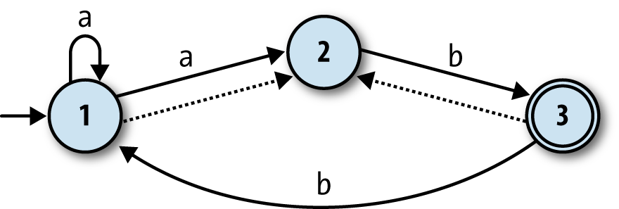
It’s possible for this NFA to be in state 1 or state 2 before it has read any input (state
1 is the start state, and state 2 is reachable via a free move), so the simulation will begin
in a state we can call “1 or 2.” From this starting point the simulation will end up in
different states depending on whether it reads a or
b:
If it reads an
a, the simulation will remain in state “1 or 2”: when the NFA’s in state 1 it can read anaand either follow the rule that keeps it in state 1 or the rule that takes it into state 2, while from state 2, it has no way of reading anaat all.If it reads a
b, it’s possible for the NFA to end up in state 2 or state 3—from state 1, it can’t read ab, but from state 2, it can move into state 3 and potentially take a free move back into state 2—so we’ll say the simulation moves into a state called “2 or 3” when the input isb.
By thinking through the behavior of a simulation of the NFA, we’ve begun to construct a state machine for that simulation:
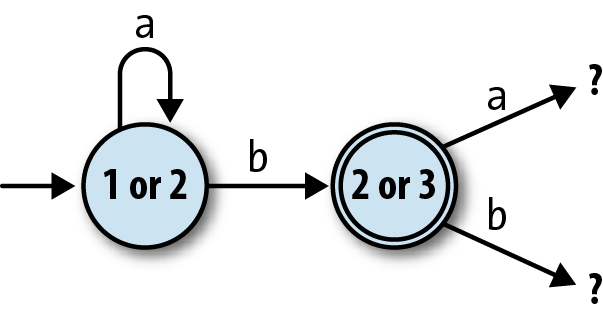
Note
“2 or 3” is an accept state for the simulation, because state 3 is an accept state for the NFA.
We can continue this process of discovering new states of the simulation until there are
no more to discover, which must happen eventually because there are only a limited number of
possible combinations of the original NFA’s states.[27] By repeating the discovery process for our example NFA, we find that there are
only four distinct combinations of states that its simulation can encounter by starting at “1
or 2” and reading sequences of as and bs:
| If the NFA is in state(s)… | and reads the character… | it can end up in state(s)… |
| 1 or 2 | a | 1 or 2 |
b | 2 or 3 | |
| 2 or 3 | a | none |
b | 1, 2, or 3 | |
| None | a | none |
b | none | |
| 1, 2, or 3 | a | 1 or 2 |
b | 1, 2, or 3 |
This table completely describes a DFA, pictured below, that accepts the same strings as the original NFA:
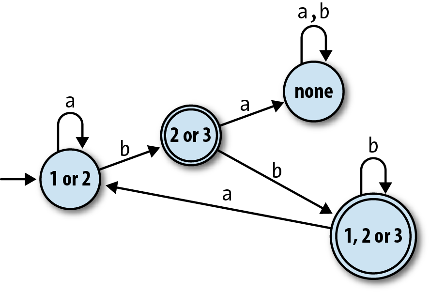
Note
This DFA only has one more state than the NFA we started with, and for some NFAs, this
process can produce a DFA with fewer states than the original machine.
In the worst case, though, an NFA with n states may require a DFA with
2n states, because there are a total of
2n possible combinations of n states—think
of representing each combination as a different n-bit number, where the
nth bit indicates whether state
n is included in that combination—and the simulation might need to be
able to visit all of them instead of just a few.
Let’s try implementing this NFA-to-DFA conversion in Ruby. Our
strategy is to introduce a new class, NFASimulation, for collecting information about
the simulation of an NFA and then assembling that information into a DFA.
An instance of NFASimulation can be
created for a specific NFADesign and
will ultimately provide a #to_dfa_design method for converting it to an
equivalent DFADesign.
We already have an NFA class that
can simulate an NFA, so NFASimulation
can work by creating and driving instances of NFA to find out how they respond to all possible
inputs. Before starting on NFASimulation, let’s go back to NFADesign and add an optional “current states”
parameter to NFADesign#to_nfa so that
we can build an NFA instance with any
set of current states, not just the NFADesign’s start state:
classNFADesigndefto_nfa(current_states=Set[start_state])NFA.new(current_states,accept_states,rulebook)endend
Previously, the simulation of an NFA could only begin in its start state, but this new parameter gives us a way of jumping in at any other point:
>>rulebook=NFARulebook.new([FARule.new(1,'a',1),FARule.new(1,'a',2),FARule.new(1,nil,2),FARule.new(2,'b',3),FARule.new(3,'b',1),FARule.new(3,nil,2)])=> #<struct NFARulebook rules=[…]>>>nfa_design=NFADesign.new(1,[3],rulebook)=> #<struct NFADesign start_state=1, accept_states=[3], rulebook=…>>>nfa_design.to_nfa.current_states=> #<Set: {1, 2}>>>nfa_design.to_nfa(Set[2]).current_states=> #<Set: {2}>>>nfa_design.to_nfa(Set[3]).current_states=> #<Set: {3, 2}>
Note
The NFA class automatically takes account of free
moves—we can see that when our NFA is started in state 3, it’s already possible for it to be
in state 2 or 3 before it has read any input—so we won’t need to do anything special in
NFASimulation to support them.
Now we can create an NFA in any set of possible states, feed it a character, and see what
states it might end up in, which is a crucial step for converting an NFA into a DFA. When our
NFA is in state 2 or 3 and reads a b, what states can it be
in afterward?
>>nfa=nfa_design.to_nfa(Set[2,3])=> #<struct NFA current_states=#<Set: {2, 3}>, accept_states=[3], rulebook=…>>>nfa.read_character('b');nfa.current_states=> #<Set: {3, 1, 2}>
The answer: state 1, 2, or 3, as we already discovered during the
manual conversion process. (Remember that the order of elements in a
Set doesn’t matter.)
Let’s use this idea by creating the NFASimulation class
and giving it a method to calculate how the state of the simulation will change in response to
a particular input. We’re thinking of the state of the simulation as being the current set of
possible states for the NFA (e.g., “1, 2, or 3”), so we can write a #next_state method that takes a simulation state and a character, feeds that
character to an NFA corresponding to that state, and gets a new state back out by inspecting
the NFA afterward:
classNFASimulation<Struct.new(:nfa_design)defnext_state(state,character)nfa_design.to_nfa(state).tap{|nfa|nfa.read_character(character)}.current_statesendend
Warning
It’s easy to get confused between the two kinds of state we’re
talking about here. A single simulation state (the state parameter of NFASimulation#next_state) is a set of many NFA
states, which is why we can provide it as NFADesign#to_nfa’s current_states argument.
This gives us a convenient way to explore the different states of the simulation:
>>simulation=NFASimulation.new(nfa_design)=> #<struct NFASimulation nfa_design=…>>>simulation.next_state(Set[1,2],'a')=> #<Set: {1, 2}>>>simulation.next_state(Set[1,2],'b')=> #<Set: {3, 2}>>>simulation.next_state(Set[3,2],'b')=> #<Set: {1, 3, 2}>>>simulation.next_state(Set[1,3,2],'b')=> #<Set: {1, 3, 2}>>>simulation.next_state(Set[1,3,2],'a')=> #<Set: {1, 2}>
Now we need a way to systematically explore the simulation states
and record our discoveries as the states and rules of a DFA. We intend to
use each simulation state directly as a DFA state, so the first step is to
implement NFASimulation#rules_for,
which builds all the rules leading from a particular simulation state by
using #next_state to discover the
destination of each rule. “All the rules” means a rule for each possible
input character, so we also define an NFARulebook#alphabet helper method to tell us
what characters the original NFA can read:
classNFARulebookdefalphabetrules.map(&:character).compact.uniqendendclassNFASimulationdefrules_for(state)nfa_design.rulebook.alphabet.map{|character|FARule.new(state,character,next_state(state,character))}endend
As intended, this lets us see how different inputs will take the simulation between different states:
>>rulebook.alphabet=> ["a", "b"]>>simulation.rules_for(Set[1,2])=> [#<FARule #<Set: {1, 2}> --a--> #<Set: {1, 2}>>,#<FARule #<Set: {1, 2}> --b--> #<Set: {3, 2}>>]>>simulation.rules_for(Set[3,2])=> [#<FARule #<Set: {3, 2}> --a--> #<Set: {}>>,#<FARule #<Set: {3, 2}> --b--> #<Set: {1, 3, 2}>>]
The #rules_for method gives us a way of exploring
outward from a known simulation state and discovering new ones, and by doing this repeatedly,
we can find all possible simulation states. We can do this with an NFASimulation#discover_states_and_rules method, which recursively finds more
states in a similar way to NFARulebook#follow_free_moves:
classNFASimulationdefdiscover_states_and_rules(states)rules=states.flat_map{|state|rules_for(state)}more_states=rules.map(&:follow).to_setifmore_states.subset?(states)[states,rules]elsediscover_states_and_rules(states+more_states)endendend
Warning
#discover_states_and_rules doesn’t care about the
underlying structure of a simulation state, only that it can be used as an argument to
#rules_for, but as programmers, we have another
opportunity for confusion. The states and more_states variables are sets of simulation states, but we know
that each simulation state is itself a set of NFA states, so states and more_states are actually
sets of sets of NFA states.
Initially, we only know about a single state of the simulation: the set of possible states
of our NFA when we put it into its start state. #discover_states_and_rules explores outward from this starting point, eventually
finding all four states and eight rules of the simulation:
>>start_state=nfa_design.to_nfa.current_states=> #<Set: {1, 2}>>>simulation.discover_states_and_rules(Set[start_state])=> [#<Set: {#<Set: {1, 2}>,#<Set: {3, 2}>,#<Set: {}>,#<Set: {1, 3, 2}>}>,[#<FARule #<Set: {1, 2}> --a--> #<Set: {1, 2}>>,#<FARule #<Set: {1, 2}> --b--> #<Set: {3, 2}>>,#<FARule #<Set: {3, 2}> --a--> #<Set: {}>>,#<FARule #<Set: {3, 2}> --b--> #<Set: {1, 3, 2}>>,#<FARule #<Set: {}> --a--> #<Set: {}>>,#<FARule #<Set: {}> --b--> #<Set: {}>>,#<FARule #<Set: {1, 3, 2}> --a--> #<Set: {1, 2}>>,#<FARule #<Set: {1, 3, 2}> --b--> #<Set: {1, 3, 2}>>]]
The final thing we need to know for each simulation state is whether it should be treated as an accept state, but that’s easy to check by asking the NFA at that point in the simulation:
>>nfa_design.to_nfa(Set[1,2]).accepting?=> false>>nfa_design.to_nfa(Set[2,3]).accepting?=> true
Now that we have all the pieces of the simulation DFA, we just need an NFASimulation#to_dfa_design method to wrap them up neatly as an
instance of DFADesign:
classNFASimulationdefto_dfa_designstart_state=nfa_design.to_nfa.current_statesstates,rules=discover_states_and_rules(Set[start_state])accept_states=states.select{|state|nfa_design.to_nfa(state).accepting?}DFADesign.new(start_state,accept_states,DFARulebook.new(rules))endend
And that’s it. We can build an NFASimulation instance
with any NFA and turn it into a DFA that accepts the same strings:
>>dfa_design=simulation.to_dfa_design=> #<struct DFADesign …>>>dfa_design.accepts?('aaa')=> false>>dfa_design.accepts?('aab')=> true>>dfa_design.accepts?('bbbabb')=> true
Excellent!
At the beginning of this section, we asked whether the extra features of NFAs let us do anything that we can’t do with a DFA. It’s clear now that the answer is no, because if any NFA can be turned into a DFA that does the same job, NFAs can’t possibly have any extra power. Nondeterminism and free moves are just a convenient repackaging of what a DFA can already do, like syntactic sugar in a programming language, rather than new capabilities that take us beyond what’s possible within the constraints of determinism.
It’s theoretically interesting that adding more features to a simple machine didn’t make it fundamentally any more capable, but it’s also useful in practice, because a DFA is easier to simulate than an NFA: there’s only a single current state to keep track of, and a DFA is simple enough to implement directly in hardware, or as machine code that uses program locations as states and conditional branch instructions as rules. This means that a regular expression implementation can convert a pattern into first an NFA and then a DFA, resulting in a very simple machine that can be simulated quickly and efficiently.
[20] This design is general enough to accommodate different kinds of machines and rules, so we’ll be able to reuse it later in the book when things get more complicated.
[21] A finite automaton has no record of its own history and no storage aside from its current state, so two identical machines in the same state are interchangeable for any purpose.
[22] This NFA actually accepts any string of a
characters except for the single-character string 'a'.
[23] Technically speaking, this process computes a fixed point of the “add more states by following free moves” function.
[24] In this simple case, we could get away with just turning the original start state
into an accept state instead of adding a new one, but in more complex cases (e.g.,
(a*b)*), that technique can produce a machine that
accepts other undesirable strings in addition to the empty string.
[25] RE2’s tagline is “an efficient, principled regular expression library,” which is difficult to argue with.
[26] Although an NFA only has one start state, free moves can make other states possible before any input has been read.
[27] The worst-case scenario for a simulation of a three-state NFA is “1,” “2,” “3,” “1 or 2,” “1 or 3,” “2 or 3,” “1, 2, or 3” and “none.”
[28] Solving this graph isomorphism problem requires a clever algorithm in itself, but informally, it’s easy enough to look at two machine diagrams and decide whether they’re “the same.”