
Chapter 26. GD and L-Systems
(Or, how to see plants on your computer without getting soil on the keyboard.)
In GD-Graph3d, you learned how Perl could create three-dimensional graphics. Naturally, Perl is quite comfortable with two-dimensional images as well. Lincoln Stein’s GD module (based on Thomas Boutell’s gd library and available from the CPAN) makes it possible to import, manipulate, and even generate GIFs from the comfort of your very own Perl. In this article, we’ll use GD to create images of plants using mathematical constructs called L-systems.
GD
Using GD is straightforward: all that’s necessary to create a GIF suitable for displaying on a web page is a GD::Image object, some colors, and a few drawing commands. It takes only six lines of code to produce a lone brown dot on a white background, a work surely worth millions to a sufficiently avant-garde patron of the arts:
#!/usr/bin/perl

use GD;

$im   = new GD::Image(100,100);
$white = $im->colorAllocate(255, 255, 255);
$brown = $im->colorAllocate(128,   0,   0);

$im->setPixel(42, 17, $brown);

open (OUT, ">masterpiece.gif") or die $!;
print OUT $im->gif();
Here we create an image 100 pixels square and allocate two colors. GIFs use color tables (in particular, a 256-color palette) so it’s necessary to specify in advance which colors are to be used. The colors themselves are specified by their red, green, and blue components, which range from 0 to 255.
The dot is then drawn with setPixel, 42
pixels to the right of the edge and 17 pixels below the top left
corner. Finally, the contents of the GIF itself, obtained through the
GD::Image::gif method, is printed to the file
masterpiece.gif.
GD provides other drawing commands, special brushes and patterns, and the ability to load existing GIFs from files. But we already have everything we need. The rest of this article is devoted to using GD to build and use code that implements L-systems, a task that proves quite comfortable in Perl, because it requires both graphical output and text manipulation.
L-Systems
For our purposes, an L-system is simply a very abstract way of modeling cell-scale growth within a plant. Bear in mind that the level of abstraction is quite high—an L-system won’t tell you much about how real plants grow. Real plant growth depends on cytoplasm structure, cell membranes, mitosis rates, and plenty of other hard-to-model phenomena. However, L-systems are quite good at generating realistic images of plants.
Originally developed by Astrid Lindenmayer (hence the ‘L’) in the late 1960’s, L-systems have undergone a number of generalizations and improvements in the decades since, including the addition of randomness, multiple transition tables, and non-discrete evolution. The core of the idea is quite simple: take a string, called the axiom, and apply a series of rules to each character of the string. For example, suppose your axiom (commonly designated ω) is A and you have two production rules:
Every A is translated to BA, and
Every B is translated to AB.
This system would be written in L-system notation as:
ω: A |
p1: A ->
BA |
p2: B ->
AB |
These rules are applied simultaneously to the axiom, producing
BA, since we start with A and
change according to rule p1. The rules are then
applied to that result, yielding ABBA (no relation
to the band). Then the rules are applied again, generating
BAABABBA.
When does the process stop? It doesn’t. In principle, the combination of axiom and rules describes an infinite sequence of words:
A
BA
ABBA
BAABABBA
ABBABAABBAABABBA
BAABABBAABBABAABABBABAABBAABABBA
and so on. This might seem to have little relevance to plant development. However, the output of an L-system can be interpreted as the shape of the plant at various ages. Finding the appropriate time to stop, then, is equivalent to deciding how big or old a tree (or fern, or flower, or blue-green algae colony) you want.
How could an L-system resemble a tree, then? To get branches we
can use a bracketed L-system. That just means
that we add [ and ] to our
L-system’s alphabet. Any string enclosed in brackets is interpreted as
separate branch, protruding from the string it would otherwise be part
of. Brackets can also be nested. For example,
A[B][CD[E[F]G]H] can be loosely interpreted as
Figure 26-1.
![A[B][CD[E[F]G]H]](http://imgdetail.ebookreading.net/software_development/2/9781449398590/9781449398590__web-graphics__9781449398590__httpatomoreillycomsourceoreillyimages688113.png.jpg)
Turtles
Typically, objects modeled with L-systems are rendered with turtle graphics. Turtle graphics were invented for the LOGO programming language; they’re used to give children a simple metaphor for expressing graphics algorithmically. Implementations of LOGO have virtual turtles that turn, move, and leave trails across the screen. Older versions sometimes had an actual robot controlled by the program. The robot moved a pen around on paper and was sometimes fashioned to look like a small, plastic-shelled turtle.
The Turtle class (in the Turtle.pm module on
this book’s web site) implements simple turtle graphics. The humble
turtle can produce some striking graphics if controlled, but itself
knows little more than its position, orientation, how to turn, and how
to move forward at an angle. The most important method of the Turtle
class is forward :
sub forward {
  my $self = shift;
  my ($r, $what) = @_;
  my ($newx, $newy) = ($self->{x} + $r *  sin($self->{theta}),
                       $self->{y} + $r * -cos($self->{theta}));
  if ($what) {
      # Do something related to motion according to
      # the coderef passed in
      &$what($self->{x}, $self->{y}, $newx, $newy);
  }
      #... and change the old coordinates
     ($self->{x}, $self->{y}) = ($newx, $newy);
  }
forward first uses a bit of trigonometry to
calculate the (x, y ) position given the distance
r and angle Θ. (All angles are measured in
radians, with zero being directly up and angles increasing as you move
clockwise.). Then it does something with the old and new coordinates,
but exactly what it does is up to $what. Whoever
calls Turtle::forward passes in a code reference;
that coderef gets the turtle’s old and new coordinates as parameters
and can do whatever it wants with them. For now, all we want the
turtle to do while moving forward is draw a line, but
this flexibility will prove quite handy later. Another method worth
examining is turn:
sub turn {
  my $self   = shift;
  my $dtheta = shift;
  $self->{theta} += $dtheta * $self->{mirror};
}
Our turtle will occasionally need to turn left into right
and right into left; this is accomplished by calling the turtle’s
mirror method; that toggles the
mirror attribute between 1 and –1 and has the
effect of changing clockwise rotations into counterclockwise
rotations.
A Turtle Draws a Tree
A turtle can’t do much by itself. Starting with a subroutine in
lsys.pl, we’ll make it more useful. To get an
L-system rule to tell the turtle what to do, we create a turtle, an
image, and a hash to translate characters into behavior:
sub lsys_init {
    # S => Step Forward
    # - => Turn Counter-clockwise
    # + => Turn Clockwise
    # M => Mirror
    # [ => Begin Branch
    # ] => End Branch
    %translate=(
                'S' => sub { $turtle->forward($changes->{"distance"},
                                              $changes->{"motionsub"}) },
                '-' => sub { $turtle->turn(-$changes->{"dtheta"}) },
                '+' => sub { $turtle->turn($changes->{"dtheta"}) },
                'M' => sub { $turtle->mirror() },
                '[' => sub { push(@statestack, [$turtle->state( )]) },
                ']' => sub { $turtle->setstate(@{pop(@statestack)}) },
               );
   my ($imagesize) = @_;

   # Create the main image
   $im = new GD::Image($imagesize, $imagesize);

   # Allocate some colors for it
   $white       = $im->colorAllocate(255, 255,255);
   $dark_green  = $im->colorAllocate(  0, 128,  0);
   $light_green = $im->colorAllocate( 0, 255,  0);

   # Create the turtle, at the midpoint of the bottom
   # edge of the image, pointing up.
   $turtle = new Turtle($imagesize/2, $imagesize, 0, 1);
}
To have the turtle perform the action identified by the
character $chr, we just say
&{$translate{$chr}}, which calls the
appropriate anonymous subroutine.
$changes, the hash reference inside
%translate, holds information specific to a given
L-system rule. It’ll go in a separate file,
tree.pl, whose beginning is shown below.
#!/usr/bin/perl

require "lsys.pl";

# Set some parameters
$changes = {  distance => 40,
                dtheta => 0.2,
             motionsub => sub { $im->line(@_, $dark_green) } };
The first two keys of the hash referred to by
$changes are straightforward:
distance is how far the turtle moves every instance
of S, and dtheta is how much the
turtle’s angle changes for every + or
-. The last key, motionsub,
identifies the anonymous subroutine passed to
Turtle::forward. Recall that
Turtle::forward passes the old position and the new
position of the turtle. sub{ $im->line(@_, $dark_green);
} merely takes that argument list, tacks on
$dark_green, and hands everything off to
GD::Image’s line method. That draws the
line.
Now we have a turtle that can turn, flip, go forward, and trace
a line. Only the left and right bracket characters remain—they’ll help
the turtle remember a position and later recall where it was. The
[ character pushes the turtle’s current state
(x, y, q, and mirror ) onto a
stack, @statestack. The ]
character, conversely, pops an element off
@statestack and forces the turtle back into that
state.
Putting L-Systems to Work
To create an honest-to-goodness L-system inside all this mess, we just need one more hash table to describe the production rules and a scalar initialized with the axiom. Let’s start with a small system:
ω: A |
p1: A ->
S[-A][+A] |
This system has every A go forward
(S ) and produce two branches, each with an
A : one to the left ([-A] ), and
one to the right ([+A] ). On every iteration, the
tree will split in half, yielding a binary tree growing upward from
the turtle’s initial location. This L-system is expressed in Perl, as
follows:
%rule  = ( A => 'S[-A][+A]' );
$axiom = "A";
%rule contains the single rule of our
L-system; $axiom is our start string. The
lsys_execute subroutine, in
lsys.pl on the book web site, applies the rules to
the axiom $repetitions times:
sub lsys_execute {
    my ($string, $repetitions, $filename, %rule) = @_;
    # Apply the %rule to $string, $repetitions times,
    # and print the result to $filename
    for (1..$repetitions) {
        $string =~ s/./defined ($rule{$&}) ? $rule{$&} : $&/eg;
    }
…and calls the appropriate subroutines held in
%translate…
foreach $cmd (split(//, $string)) {
    if ($translate{$cmd}) {&{$translate{$cmd}}( );}
}
…and finally prints out the GIF itself:
 open (OUT, ">tree.gif") or die $!;
 print OUT $im->gif;
 close(OUT);
}
This program creates the GIF shown in Figure 26-2.
#!/usr/bin/perl

require "lsys.pl";

%rule = ( 'A' => 'S[-A][+A]', );
$axiom = "A";

$changes = { distance => 40,
               dtheta => 0.2,
            motionsub => sub { $im->line(@_, $dark_green) } };

$repetitions = 8;
$imagesize   = 400;
$filename    = "tree1.gif";

lsys_init($imagesize);
lsys_execute($axiom, $repetitions, $filename, %rule);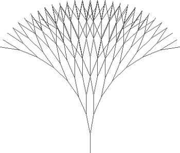
Not breathtaking, but moderately tree-like. Its most glaring
flaw is that all the branches are the same length. Younger branches
should be shorter, because they’ve had less time to grow. Changing the
system makes every G produce an
S at every step.
ω: A |
p1: A ->
GS[-A][+A] |
p2: G ->
GS |
Here’s the program to code the rule in Perl and shorten the distance a bit:
#!/usr/bin/perl

require "lsys.pl";

%rule  = ( 'A' => 'GS[-A][+A]', 'G' => 'GS' );
$axiom = "A";

$changes = { distance => 10,
               dtheta => .2,
            motionsub => sub { $im->line(@_, $dark_green) } };

$repetitions = 8;
$imagesize   = 400;
$filename    = "tree2.gif";

lsys_init($imagesize);
lsys_execute($axiom, $repetitions, $filename, %rule);
This produces the tree shown in Figure 26-3.
A definite improvement. However, most plants aren’t perfectly symmetrical. Let’s try forcing the right branch to wait before splitting. Specifically, we’ll use this L-system:
ω: A |
p1: A ->
GS[-A][+B] |
p2: G ->
GS |
p3: B ->
C |
p4: C ->
A |
Now every right branch spends less time splitting and growing. Here’s the program that implements this system:
#!/usr/bin/perl

require "lsys.pl";

%rule = ('A' => 'GS[-A][+B]',
         'G' => 'GS',
         'B' => 'C',
         'C' => 'A'),

$axiom   = "A";
$changes = { distance => 2.8,
               dtheta => .2,
            motionsub => sub { $im->line(@_, $dark_green) } };

$repetitions = 15;
$imagesize   = 400;
$filename    = "tree3.gif";

lsys_init($imagesize);
lsys_execute($axiom, $repetitions, $filename, %rule);
The result is shown in Figure 26-4.
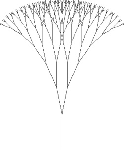
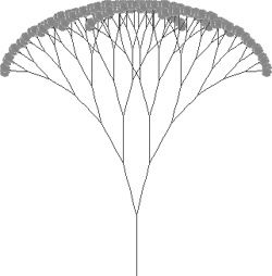
Interesting, but kind of lopsided. Remember Turtle’s
mirror method? Now’s a good time to take advantage
of it. Let’s try changing the first rule of the L-system to
p1: A ->
GS[---A][++MB] |
and decreasing dtheta a bit:
#!/usr/bin/perl

require "lsys.pl";

%rule = ('A' => 'GS[---A][++MB]',
         'G' => 'GS',
         'B' => 'C',
         'C' => 'A'),

$axiom   = "A";
$changes = { distance => 2.8,
               dtheta => .06,
            motionsub => sub { $im->line(@_, $dark_green) } };

$repetitions = 15;
$imagesize   = 400;
$filename    = "tree4.gif";

lsys_init($imagesize);
lsys_execute($axiom, $repetitions, $filename, %rule);
The tree produced by this program is shown in Figure 26-5. Now the second branch of every subtree is flipped, and the tree looks less like the victim of gale-force winds.
Merely drawing branches may be good enough for trees in winter, but around this time of year, plants acquire things that are harder to draw: leaves and flowers. Fortunately, GD can draw and fill polygons and import other GIFs.
Leaves
Our leaves will be polygons oriented in some direction relative
to the branch they’re on. We’ll use the already-existing turtle code
and create a “polygon mode,” using the traditional L-system notation
of curly braces. The turtle will trace out the polygon and then fill
it. Turtle::forward can perform any sort of
movement as long as we pass it the appropriate coderef—we just need to
construct one that tells GD to convert part of the turtle’s path into
polygon vertices.
It would be convenient to modify distance and
dtheta in polygon mode independently of their
values in “stem mode.” Since these two values are stored in
%$changes, we’ll create two hashes:
%stemchanges for stem mode, and
%polychanges for polygon mode.
$changes will always be current whatever the mode,
so it’ll initially refer to %stemchanges. The most
important difference between them is their
motionsub ; %stemchanges has the
familiar sub { $im->line(@_, $dark_green) }, but
%polychanges has sub {
$poly->addPt(@_[0..1]) }.
Skipping what that means for the moment, let’s handle curly
braces with two more entries to %translate :
%translate = (...
              '{' => sub {    $poly = new GD::Polygon;
                           $changes = \%polychanges;    },

              '}' => sub { $im->filledPolygon($poly, $light_green);
                           undef $poly;
                           $changes = \%stemchanges;    } );
What’s going on? The GD module defines the GD::Polygon class, an
instance of which $poly gets created whenever we
encounter a {. Every time the turtle moves in
polygon mode, $polychanges{motionsub} is called, so
we call GD::Polygon::addPt to add a point to the
list of vertices in $poly. Once the polygon is
drawn, a } is processed, filling the polygon with
$light_green. Then $poly is
thrown away and stem mode is restored.
#!/usr/bin/perl

require "lsys.pl";

%rule  = ( 'A' => 'SLMA', 'L' => '[{S+S+S+S+S+S}]'),
$axiom = "A";

%stemchanges = ( distance => 24,
                   dtheta => .15,
                motionsub => sub{ $im->line(@_, $dark_green) } );

%polychanges = ( distance => 6,
                   dtheta => .4,
                 motionsub => sub{ $poly->addPt(@_[0..1]) } );

$changes     = \%stemchanges;
$repetitions = 15;
$imagesize   = 400;
$filename    = "tree5.gif";

lsys_init($imagesize);
lsys_execute($axiom, $repetitions, $filename, %rule);
The result (Figure 26-6) resembles a vine.
This system is pretty easy to follow—it merely leaves commands
for moving forward, drawing a leaf, and flipping the turtle, repeated
an arbitrary number of times. The M character once
again proves useful, this time allowing easy alternating placement of
leaves. Also note that GD automatically closes polygons if they’re not
closed already.
Flowers
Let’s use some GIFs of flowers: flower.gif,
flower2.gif, and flower3.gif,
all available on the book web site. Creating a GD::Image from an existing file is easy—the
newFromGif method does exactly that. All you need
to add to lsys_init is the following:
open(IN, "flower.gif") or die $!;
$flower = newFromGif GD::Image(IN);
close(IN);

open(IN, "flower2.gif") or die $!;
$flower2 = newFromGif GD::Image(IN);
close(IN);

open(IN, "flower3.gif") or die $!;
$flower3 = newFromGif GD::Image(IN);
close(IN);
Once all the flowers are loaded, we need to copy them onto the
main image. We’ll delegate that to a small subroutine in
lsys.pl, which centers the image at the turtle’s
current coordinates. It uses GD::Image’s getBounds
method:
sub flower {
    my $flower=shift;
    my ($width, $height) = $flower->getBounds( );
    my ($x, $y) = $turtle->state( );
    $im->copy($flower, $x-$width/2, $y-$height/2, 0, 0, $width, $height);
}
GD::Image::copy does the dirty work here,
even copying the flowers’ color tables if necessary. We’ll add a few more
entries to %translate :
%translate = (...
              'f' => sub { flower($flower)  },
              'g' => sub { flower($flower2) },
              'h' => sub { flower($flower3) } );
We can test the new features with this program:
#!/usr/bin/perl
require "lsys.pl";
%rule = ( 'A' => 'GS[-fA][+fA]', 'G' => 'GS'),
$axiom = "A";
%stemchanges = ( distance => 9,
dtheta => .25,
motionsub => sub{ $im->line(@_, $dark_green) } );
%polychanges = ( distance => 6,
dtheta => .4,
motionsub => sub{ $poly->addPt(@_[0..1]) } );
$changes = \%stemchanges;
$repetitions = 8;
$imagesize = 400;
$filename = "tree6.gif";
lsys_init($imagesize);
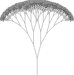
lsys_execute($axiom, $repetitions, $filename, %rule);Now our tree has flowers, as shown in Figure 26-7.
It looks odd with flowers growing out of every branch. One way to avoid this is forcing flowers to die every step, leaving live flowers only at the very tips:
#!/usr/bin/perl

require "lsys.pl";

%rule  = ('A'=>'GS[-fA][+fA]', 'G'=>'GS', 'f'=>''),
$axiom = "A";

%stemchanges = ( distance => 9,
                   dtheta => .25,
                motionsub => sub { $im->line(@_, $dark_green) } );

%polychanges = ( distance => 6,
                   dtheta => .4,
                motionsub => sub { $poly->addPt(@_[0..1]) } );

$changes     = \%stemchanges;
$repetitions = 8;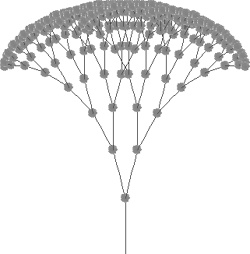
$imagesize   = 400;
$filename    = "tree7.gif";

lsys_init($imagesize);
lsys_execute($axiom, $repetitions, $filename, %rule);
The result is shown in Figure 26-8.
Alternately, you can have the flowers change before they die:
#!/usr/bin/perl

require "lsys.pl";

%rule  = ('A' => 'GS[-fA][+fA]', 'G' => 'GS', 'f' => 'g', 'g' => 'h', 'h' => ''),
$axiom = "A";

%stemchanges = ( distance => 9,
                   dtheta => .25,
                motionsub => sub { $im->line(@_, $dark_green) } );

%polychanges = ( distance => 6,
                   dtheta => .4,
                motionsub => sub { $poly->addPt(@_[0..1]) } );

$changes     = \%stemchanges;
$repetitions = 8;
$imagesize   = 400;
$filename    = "tree8.gif";

lsys_init($imagesize);
lsys_execute($axiom, $repetitions, $filename, %rule);
Figure 26-9 shows the changed flowers.
Bringing It All Together
The L-system itself is an incredible source of variety; even the primitive system I’ve presented is still capable of making appealing pictures. For a few final examples, we’ll experiment with some additional rules. Using just one type of flower:
#!/usr/bin/perl
require "lsys.pl";
%rule = ('A' => 'GS[---fMA][++++B]',
         'B' => 'C',
         'C' => 'GS[-fB][++A][++++A]',
         'f' => '',
         'G' => 'HS',
         'H' => 'HSS'),

$axiom = "A";

%stemchanges = ( distance => 4,
                   dtheta => 0.12,
                motionsub => sub { $im->line(@_, $dark_green) } );

%polychanges = ( distance => 6,
                   dtheta => 0.4,
                motionsub => sub { $poly->addPt(@_[0..1]) } );

$changes     = \%stemchanges;
$repetitions = 10;
$imagesize   = 400;
$filename    = "tree9.gif";

lsys_init($imagesize);
lsys_execute($axiom, $repetitions, $filename, %rule);
The result is illustrated in Figure 26-10.
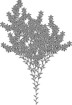
With leaves and a different flower:
#!/usr/bin/perl
require "lsys.pl";
%rule = ( 'A' => 'S[---LMA][++++B]',
          'B' => 'S[++LBg][--Cg]',
          'C' => 'S[-----LB]GS[+MC]',
          'g' => '',
          'L' => '[{S+S+S+S+S+S}]' );

$axiom = "A";
%stemchanges = ( distance => 18.5, dtheta => 0.1,
                motionsub => sub { $im->line(@_, $dark_green) } );

%polychanges = ( distance => 3, dtheta => 0.4,
                motionsub => sub { $poly->addPt(@_[0..1]) } );

$changes     = \%stemchanges;
$repetitions = 10;
$imagesize   = 400;
$filename    = "tree10.gif";

lsys_init($imagesize);
lsys_execute($axiom, $repetitions, $filename, %rule);
This gives us a bush (Figure 26-11).
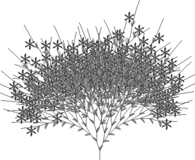
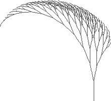
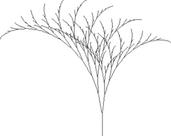
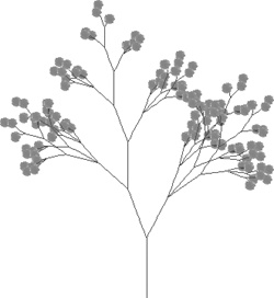
With all three flower types, leaves, and slightly weird axial growth, use this program:
#!/usr/bin/perl

require "lsys.pl";

%rule=( 'A' => 'GS[---fA][++MB]',
        'B' => 'C',
        'C' => 'A',
        'f' => 'g',
        'g' => 'h',
        'h' => '',
        'G' => 'HS',
        'H' => 'IS',
        'I' => 'GLMS',
        'L' => '[{S+S+S+S+S+S}]' );

$axiom = "A";
%stemchanges = ( distance => 2.8, dtheta => 0.06,
                motionsub => sub { $im->line(@_, $dark_green) } );

%polychanges = ( distance => 3, dtheta => 0.4,
                 motionsub => sub { $poly->addPt(@_[0..1]); } );

$changes     = \%stemchanges;
$repetitions = 17;
$imagesize   = 400;
$filename    = "tree11.gif";

lsys_init($imagesize);
lsys_execute($axiom, $repetitions, $filename, %rule);
Figure 26-12 depicts our final L-system-generated tree.
Resources
You can find several L-systems programs for Unix, Macs, and DOS platforms at http://www.cpsc.ucalgary.ca/projects/bmv/software.html. If you don’t mind peeling your eyes off the monitor, the definitive text on L-systems is The Algorithmic Beauty of Plants, by Lindenmayer and Prusinkiewicz (Springer-Verlag, 1990).