11 Test Metrics

Test metrics allow quantitative statements regarding the quality of a product and its development and test processes. They must therefore be built on solid measurement theoretical foundations. Metrics form the basis for transparent and traceable test process planning and control. Based on different measurement objects, we can create test-case-based metrics, test-basis and test-object-based metrics, defect-based metrics, and cost- and effort-based metrics. One added value of such metrics is that statements can be made regarding the best possible test finishing date, using on the one hand experienced-based estimates on the probability of residual defects and on the other hand statistical failure data analysis and reliability growth models.

11.1 Introduction

Performing test management activities such as test process planning and control or test end evaluation, qualitative statements such as “We must do extensive testing” are by no means sufficient. On the contrary, required are quantitative and objectively verifiable statements such as “All components from safety requirement level 2 onward must be component tested with 100% branch coverage”. This is also reflected, for instance, in the Capability Maturity Model Integration (CMMI [CMMI 01], see chapter 7) and the ISO 9000 family of standards, which require quantitative statements about planning and control.

However, how do test managers obtain quantitative statements or specifications regarding products and processes? The answer is, they do it in the same way as, for example, someone specifying the floor area or the wall thickness of a new house—through measurement values.

And how do we verify that the specifications have been met? Through measurement! In Software Testing Foundations, it was explained that quality attributes can be measured with measurement values or metrics and that McCabe’s cyclomatic complexity metric can be taken as a possible measure for the evaluation of program code complexity ([Spillner 07, section 4.2.5]).

Hence, evaluation and measurement are central test management activities and must be put on sound theoretical foundations. The most important ones are explained in section 11.2. Section 11.3 describes how metrics are defined and evaluated, and section 11.4 shows how measurement values can be visualized by means of graphs and diagrams. Based on this, section 11.5 sets out to describe the most important test metrics. Section 11.6 deals with residual defect and reliability estimations.

Measure

11.2 Some Measure Theory

A measurement is generally understood as a number of symbols, identifiers, or figures that can be assigned to specific features of a (measurement) object by means of a measurement specification.

Measurements relate features of objects to values.

Observations on objects can be carried out with or without technical aids. If technical means are used, we talk about a →measurement. In most cases, measurement in the technical, physical sense means comparing and assigning measurement values. Going back to the previous example, the thickness of a wall can be compared with the values of a measuring system, for example, a yardstick or a tape measure. The measurement value is expressed as a number and unit, e.g., 25 cm or 250 mm.

If a measurement relates directly to an object or its features, we talk about a direct measurement; otherwise, we talk about a derived measurement. A derived measurement cannot directly measure the feature that is in the focus of our interest but instead measures one or several directly measurable features that we assume bear a specific relation to the feature we are focusing on.

Measurements can be direct or derived.

Often, indirect measurements are formulated with the aid of models that help to explicitly express the relation to the actual measurement object or features that we are interested in.

Models for indirect measurements

In the first instance, information gained through indirect measurements is valid only within the context of our model assumptions, and the quality of the interpretation or transfer of such information from the model back to the real world is dependent on the quality of the model.

For instance, if in our house-building example a model such as the architectural drawing is not to scale, we cannot infer from measurements taken from the drawing that one room is “larger” than another.

Instead of the general term “measurement”, we sometimes casually speak of “metrics”—Greek μ, (the art of) meter, relating to measurement. In mathematics, this term is defined as a function that describes the “distance” between two elements of an arbitrary (vector-)space. For example, the Euclidian distance between two points a and b with the Cartesian coordinates x_a, y_a and x_b, y_b is formulated as a function

Measurement = metric?

d(a, b) = √[(x_a – x_b)² + (y_a – y_b)²]

and is a metric in the mathematical sense.

In software engineering and in testing, the term “metric” is used for both the measurement techniques and the measurements values used to measure certain features of the measurement objects. The IEEE standard 1061 ([IEEE 1061]) defines a software (quality) metric as a function that maps specific properties of software development processes, or of interim or end products, to values of a predefined value range. The resulting values or value combinations are interpreted as the degree of fulfillment of specific (quality) features.

In software engineering metric is used to denote measurement as well as measurement techniques.

Measurement objects, therefore, are software development projects or underlying processes (figure 11-1a) or concrete products such as a program text, design model, test case, etc. (figure 11-1b).

Figure 11–1 Measurement and measure

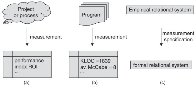
Generally speaking, a measurement relates specific features of objects of a so-called empirical relational system¹ (e.g., some property of a software artifact) to specific values of a formal relational system (e.g., the natural numbers, by means of a measurement specification).

An empirical relational system, for instance, can be the number of all programs written in a particular programming language together with the attribute “comprehensibility.” A possible measurement counts the lines of code, and the associated formal relational system consists of the (value) set of the natural numbers 0, 1, 2 ... and the larger-than-or-equal-to relation. The measurement values are then interpreted as “a larger value corresponds to lesser comprehensibility”.

A measure (or metric) is thus made up of the following elements: an empirical and a formal relational system, the measurement specification to map specific attributes of elements of the empirical relational system to values in the formal relational system, and the interpretation of the relation in the formal relational system with respect to the observed features in the empirical relational system. This general relationship is illustrated in figure 11-1c.

Measurements associate empirical with formal relational systems.

It is important to understand clearly that the results of metrics are, to begin with, hypotheses that need to be validated. It is therefore necessary to define or select metrics that are relatively simple and easy to reproduce and adequate to the project’s needs. It is equally important to continuously verify the quality and target orientation of these metrics

11.3 Metrics Definition and Selection

Metrics and metrics collections are not an end in themselves but meant to provide a quantified, objective basis for decision making. This section explains how metrics can be accurately defined and methodically selected.

Before thinking about concrete measurement objects and associated measurable features, we need to be clear in our minds about which fundamental objectives we really want to achieve and track through measurement.

Selecting suitable metrics

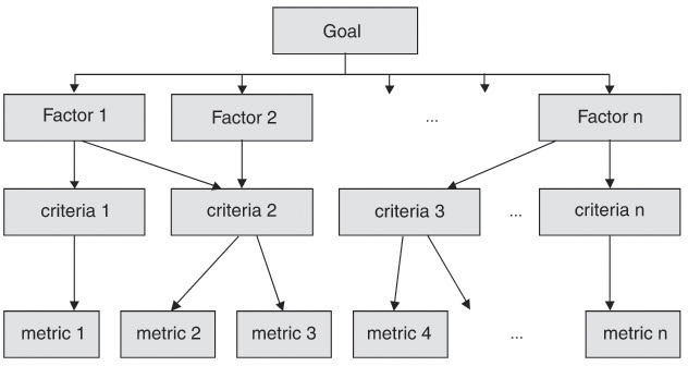
Major objectives such as quality or productivity targets are broken down into subobjectives until we can assign one or several measurement objects and a small number of practical and applicable metrics to each of them.

This method, known as the “factor-criteria-metrics” (FCM) method (see figure 11-2) forms one of the bases of the quality model of the ISO 9126 family of software-quality-related standards. There, quality attributes are broken down to subattributes and further to measurable quality factors that can be assigned to concrete metrics.

A distinction is made between internal and external metrics, the former measuring the product itself and the latter measuring attributes that can be observed during the use or operation of the product.

The ISO 9126 standard, for instance, decomposes the quality attribute “efficiency” into the subattributes “time behavior” and “resource utilization.” With regard to the subattribute “time behavior,” the external metric measures the response time T as the difference between the system’s response and the completion of the corresponding command.

Figure 11–2 Factor-criteria-metrics- (FCM) method

In order to arrive at individual factors and finally at metrics, Basili and Weiss ([Basili 84]) in their “Goal Question Metric” (GQM) method recommend starting with the definition of goals. For each goal we should then think of questions we would have to answer to see if we are reaching that goal. Roughly speaking, we must first ask what we actually want to find out. Subsequently, we construct simple hypotheses and consider which kind of data or measurement values we need to confirm or disconfirm these hypotheses.

The Goal Question Metric (GQM) method

It may, for example, be our goal to gain better control of the test process. We may want to ask, for example, the following questions: Which tasks have been completed within the planned time? Which tasks have not been completed? Which tasks are delayed? Possible measurements would, e.g., be product completeness, already used-up resources, or already agreed-upon delivery dates.

Measurement objects in test management are test basis documents (e.g., requirements and design specifications) and the test objects themselves as well as corresponding test case specifications, test scripts, and test reports. In addition, similar to the above GQM-example, the test process itself serves as a measurement object whose attributes such as progress of plan, effectiveness, and efficiency can be quantified with one or more measurements.

Measurement objects in test management

Once we are certain which attributes or factors of a measurement object are to be measured (empirical relational system), the measurement specification and the value range of the measurements (formal relational system) are defined. It is important to accurately define the so-called scale or scale type as it limits the operations allowed on the measurement values.

The scale indicates which operations are allowed with the measurement values.

If, for example, we take two programs, A and B, and measure their number of lines, with A resulting in 250) lines and B in 500 lines, we may rightly assert that B is twice as long as A. However, if program A were classified 1 (equivalent to “short”) and program B as 2 (equivalent to “medium”), it would not tell us anything about the ratios of the lengths of A and B. But if, in the latter case, test cases executed 100 lines of code each in both programs A and B, we could infer that A was structurally “better” tested than B.

Formal measure theory knows the five scales listed in table 11-1 ([Zuse 98]) and distinguishes between metric and non-metric scale types. For software measurements, we ought to look for metric scale types, since otherwise the measurement values will not (or only in a very limited fashion) be open to mathematical operations and statistical evaluations.

Table 11–1 Features of the five scale types

Scale type	Expression	Attributes/permitted operations	Possible analyses
non-metric	Nominal scale	Identifier	Comparison, median, quantile
		Renaming
	Ordinal scale	Rank value with ordinal numbers	Classification, frequencies
		All F with x ≥ y ⇒ F(x) ≥ F(y)
metric	Interval scale	Equal scale without natural zero point	Addition, subtraction, average, standard deviation
		All F with F(x) = a x x + b
	Ratio scale	Equal scale with natural zero point	Multiplication, division, geometric mean, variation
		All F with F(x) = a x x and a > 0
	Absolute scale	Natural number and measurement units	all
		Identity F(x) = x only

In the above example, the number of lines of code resembles an absolute scale, whereas the (subjective) classification would have been on a nominal scale where the values cannot be divided. The scale for the above mentioned response time metric T to measure the quality subattribute “time behavior” is of scale type “ratio scale” and has the natural zero point 0 seconds, which at the same time is its lowest value because negative response times would violate the principle of causality.

The following requirements or criteria help to evaluate the quality of measurements or metrics:

Requirements for “good” metrics

A good measurement must be easily calculable and interpretable and must correlate sufficiently with the attribute it is supposed to measure (statistical validation!).

Measurements must be reproducible; i.e., the measurement values must be objectively obtainable (without being influenced by the person taking the measurement).

Measurements must be robust against “insignificant” changes of the measurement object; i.e., the measurement value must be in a continuous functional relationship with the measured attribute.

A further requirement is the timeliness of the measurement values or measurements. Measurements must be taken early enough to enable you to make relevant decisions that can positively influence target achievement.

A question closely associated with the scale type of a measurement is whether, and how far, measurement values can be compared and statistically evaluated. Expedient in this respect are the ratio and absolute scales.

If a measurement has been successfully used in several different projects, we may, as it were, take this as empirical evidence that is has been reasonably defined and that it is usable. In the end, for reasons of documentation, all measured values must be traceable and reproducible.

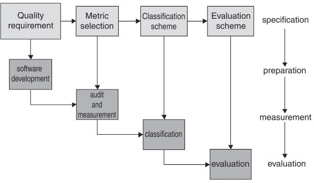
In test management (see figure 11-3), metrics are defined based on the quality requirements and incorporated in the test plan: based on the metric definitions tests are planned and designed as measurements. During execution of the tests, the test object is measured, classified into the selected classification scheme, and evaluated with regard to its quality attributes (see also section 5.2.6).

Figure 11–3 Metrics-based quality assurance

For cataloguing, distribution, and application, it is best to document metrics consistently, using the template provided in table 11-2 ([Ebert 05]).

Table 11–2 Metrics definition template

Field	Description
Name/identifier	Name or identifier (filename; ID number)
Description	Brief, succinct description
Motivation	Goals and issues that are to be accomplished or addressed
Base data	Product attributes or other metrics taken as a basis
Scale type	Scale (nominal, ordinal, interval, ratio, absolute)
Definition	Calculation algorithm
Tools	References and links to support tools
Presentation	Visualization; i.e., possible chart types
Frequency	Frequency/interval in which metric must be created
Costs	One-off, introductory costs, and regular metrics collection costs
Method of analysis	Recommended or permitted statistical operations
Target and boundary values	Specified range of values for product, project, or process evaluation
Storage location	Configuration management system, project database
Distribution	Visibility and access control
Training	Available training opportunities (training, documentation)
Examples	Application examples, including graphs and data collection

---

Templates and concrete metric definitions as well as up-to-date measurement values should be made available via an intranet, allowing all project members immediate access to associated documents, data collections, and analysis results.

---

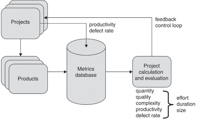
With increasing maturity level of the test processes, the selection, collection, and evaluation of metrics becomes a clearly defined test management activity. Figure 11-4 shows the metrics-based feedback loop structure for test management.

Figure 11–4 Metrics-based test management feedback

For a more detailed illustration, see [Ebert 05] and the ISO 15939:2002 standard ([ISO 15939]), which defines a software measurement process.

11.4 Presenting Measurement Values

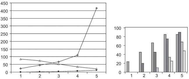
A variety of different charts or diagrams can be used to display measured values. Popular are bar or column charts to show metric values for several measurement objects (right, figure 11-5) as well as line charts to show the chronological progression of a measurement object or of one or several metrics (left, figure 11-5).

Diagrams help you to visualize measurement values and their progression.

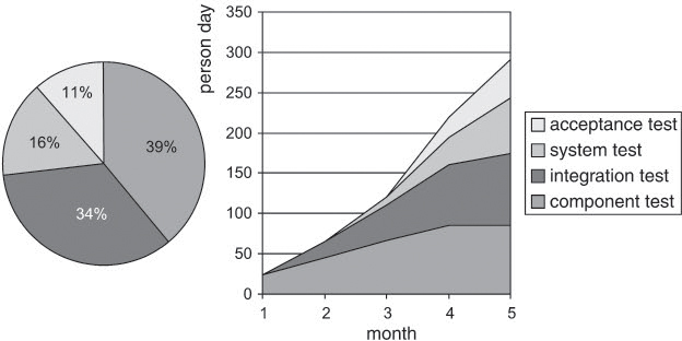
Circle or pie charts are favored for presenting portions of several measurement values or measurement objects from a certain total size onward (left, figure 11-6). Lesser known are so-called cumulative charts, which can be used to show the sum of several measurement values in their chronological progression in the form of stacked line charts.

Figure 11–5 Line and bar charts

The chart to the right in figure 11-6 shows the cumulated efforts of component testing, integration testing, and system and acceptance testing in person days. Component testing ends at the beginning of the fourth month so that allocated cumulated effort remains constant from that month onward. All in all, approximately 295 person days were spent until the fifth month.

Figure 11–6 Pie chart and cumulative chart

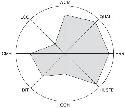
For most of the measurement objects, several metrics are collected simultaneously, each highlighting different features or aspects of the measurement object. In order to be able to evaluate a measurement object as a whole, it may not be sufficient to consider the measurement values of only one metric in isolation. It is the overall view that is of interest. As figure 11-7 illustrates, Kiviat diagrams combine measurement values of several metrics with a corresponding number of concentrically or rotation symmetrically arranged axes, each indicating the measurement value of one metric. The associated points on the axes are bounded by a closed polygon so that, with some experience, the evolving pattern can be used to deduce features of the measurement object as a whole.

Kiviat charts illustrate values of many metrics in a concise way.

---

Example: Kiviat diagram in VSR

The VSR test manager studies the Kiviat diagram illustrated in figure 11-7, showing the metric values for one class of the object-oriented implementation. The value for the weighted count of methods (WCM) is at approximately 80%, and the depth of inheritance (DIT) is 9, hence rather deep. Since the other values are relatively high, too—i.e., the values for the average complexity of the methods (CMPL), the errors found (ERR), and the Halstead metrics (HLSTD)—the test manager recommends a refactoring of the class.

Figure 11–7 Kiviat diagram

---

11.5 Several Test Metrics

After our more general discussion on measurements and metrics, this section introduces concrete →test metrics, which are useful for the measurement of the test process or the evaluation of product quality.

Test metrics can be distinguished according to the different measurement objects under consideration, resulting in the following:

Test-case-based metrics

Test-basis- and test-object-based metrics

Defect-based metrics

Cost- or effort-based metrics

As already suggested in the metrics examples above, there are many metrics in which both absolute numbers (number of tested X) and ratio values (number of tested X / number of all X) are of interest.

11.5.1 Test-Case-Based Metrics

Test-case-based metrics focus on a large number of test cases and their respective states. They are used to control progress of the test activities with reference to the test (project) plan or its different versions. Here are some examples for metrics with absolute scales:

Number of planned test cases

Number of specified test cases

Number of created test procedures

Number of test script lines

And here are a couple of examples of test-case-based metrics with ratio scales:

Number of test cases with priority 1/number of planned test cases

Number of specified test cases/number of planned test cases

During the course of a test cycle there are many instances where new test cases must be developed in addition to those planned; for instance, if particular coverage targets cannot be reached with the available test cases.

Measure the unexpected, too!

In most cases, requirement changes, too, require new tests or changes in current test cases, or even make old ones obsolete. Metrics with absolute scales are as follows:

Number of unplanned new test cases

Number of changed test cases

Number of deleted test cases

If, for example, the number of unplanned new test cases rises above a particular value, this may be an indication of insufficient requirements management. A high number of changed test cases relating to one requirement or many changes of a test case within a short period of time allows us to conclude that requirements are vague or ambiguously defined and that they will only gradually be specified more precisely during the course of the development phase.

Also interesting for test processes control are metrics concerning test execution, such as these, for instance:

Number of executed test cases (already mentioned)

Number of successfully (without failure, passed) executed test cases

Number of failed (with failure) test cases

Number of blocked test cases (not executable due to violated preconditions)

A high number of executed test cases is an indication of well-structured, largely independent test cases, whereas a high number of blocked test cases indicates that too many dependencies exist between test cases. If some of these tests fail, many subsequent test cases based on postconditions of previous ones cannot be executed either.

Of course, the number of successful or failed tests executed on the test object is not only interesting for test control, it is particularly interesting in the evaluation of product quality.

In maintenance testing or in case of new software versions in regression testing, these metrics are often separately collected for current, new, and changed test cases. Often the number of unplanned new test cases executed (with/without defect) is also collected separately.

The values of the test-case-based metrics, too, are often shown separately per test level and priority of the test cases (e.g., in cumulative diagrams).

In a wider sense, metrics on elements of the test environment (e.g., test bed with test drivers and stubs, test data, simulators, analyzers, etc.) are also classed with the test-case-based metrics. Here are a couple of useful examples:

Plan and control the test environment setup

Number of planned or available test drives or stubs

Number of planned or available lines of code per test driver or stub

Essentially, test-case-based metrics take into account all test cases specified in the test schedule. However, a hundred percent test progress in terms of test schedule does not necessarily mean that the test object has been sufficiently tested.

Consider different test coverage concepts.

Therefore, additional suitable product-oriented test coverage metrics are needed that measure test progress against the test base or the size of the test object.

The next section describes some corresponding metrics.

11.5.2 Test-Basis- and Test-Object-Based Metrics

The metrics outlined in this section are aimed at the features and coverage of the test basis and test object. Depending on test level, elements such as requirements, design elements, program code, and user manuals are measured by test metrics in relation to the test process—for instance, to measure the quality of the test case design or the progress of the test activities in relation to the size of the test object.

In code, for instance, we can measure how many lines of code or instructions were executed during testing. In case of (functional) specifications we can measure which system functions (features) were verified by the test. Based on the system architecture, we can trace which system components have been tested. Regarding the system requirements, we can trace how many requirements have been validated by tests.

To do so, it is necessary to record which requirements have been specified by whom and by means of which functional and technical design documents; furthermore, we need to document which program parts were used for the implementation of which requirements and which test cases were taken for the verification of these requirements. This information is necessary to ensure that we have bidirectional traceability from the requirement’s source to implementation and back, that they can be traced to corresponding test cases, and that we can measure the coverage.

Trace requirements

Such coverage metrics are always useful if their abstraction level correlates with the test level for which they are intended.

Depending on the requirements engineering methodology used, it is possible to collect function- or requirements-oriented coverage metrics during system and acceptance testing:

System and acceptance test: function-or requirements-based metrics

Number of tested functions/total number of functions

Number of tested dialogue/number implemented dialogues

Number of executed test cases/number of specified test cases per function

Number of tested hours per function

The application of specification-based metrics requires the traceability of requirements from the requirements to their functional and technical system design and right up to their test cases. In this case, measurements like the following can be made:

Percentage of all requirements covered by test cases

Percentage of all use case scenarios executed

Percentage of all functional classes or data types created/read/changed or deleted

Metrics must also be collected for tests regarding nonfunctional requirements:

Number of platforms covered by test

Number of localized² versions

Number of performance requirements per platform covered by test

During integration testing, special focus is put on design components and particularly on interface interaction—which and how many interfaces are there in the system and which of them have been covered by test? Metrics examples are as follows:

Integration testing: Focus on interface metrics.

Percentage of interfaces tested

Percentage of interface usage tested

Percentage of interface parameters tested with test technique XYZ

After execution of the specified test cases, all software parts not covered according to the specifications in the test plan are checked to see if test cases may possibly be missing in the test design specification. If this is the case, they will be added and the test repeated with the new test cases. One useful metric in this connection is the defect-based “test design verification” metric (see section 11.5.3).

In component testing, measurement typically focuses on structure-oriented metrics based on program code (“code coverage”). Measurable are, for example, the following:

Component testing: structure-oriented metrics

Number of new or changed functions or operations

Number of lines of code or executable instructions (kilo lines of code (KLOC) or kilo delivered source instructions (KDSI))

Code complexity (cyclomatic complexity or McCabe metric)

Number of covered paths in the control flow graph

Complexity metrics serve as product risk indicators and for risk-based control of the test effort (see chapter 9). Structure-oriented dynamic metrics such as statement coverage (C0) and branch coverage (C1) require the previous instrumentation of the programs. Appropriate instrumentation tools allow us to make measurements such as these:

Percentage of operations or procedures called

Percentage of instructions that have been executed

Percentage of branches in the control flow graph that were covered

Percentage of procedure calls that have been executed

Many other test-basis- and test-object-based metrics are found in [Kaner 95] and [Zhu 97]. Test-object- and test-basis-based metrics for object-oriented software are listed in [Winter 98] or [Zuse 98].

11.5.3 Defect-Based Metrics

Besides tracking test progress with test-case-, test-basis- and test-object-based metrics, the test manager is also asked to evaluate test results, in particular detected failures and defects, and use them for controlling the test process.

For ease of reading, we shall in the following also use the terms “defect” and “fault” for “failure”.

The IEEE Standard Dictionary of Measures of the Software Aspects of Dependability ([IEEE 982.1]) recommends, among others, the collection of the following defect-based metrics whose values are normally separately classified according to defect severity and test level:

Defect density (fault density): number of defects in relation to the size of the test object—e.g., number of defects/KLOC (or KDSI)—hence also the defect distribution as the number of defects per test object or test level, etc.

→Failure rate: the number of failures detected or expected to be detected during the execution time of a test or program

→Fault days: number of days from defect injection into the system and proof that a resulting failure has occurred

Especially in complex or distributed development projects, we often get different defect densities in different components. This is expressed in different defect detection percentages during test execution (if test quality and efficiency are the same for all components). As long as component testing has not been fully completed, we will go on to find more defects per test in components with a higher initial defect density.

In reference to values estimated earlier by the test manager (e.g., based on data of earlier projects), these metrics can also be combined with indirect metrics to measure test effectiveness (number of found failures per test) and test efficiency (number of found failures per given period of time), for instance as the following:

Indirect defect-based test metrics allow conclusions on test effectiveness and efficiency.

Defect detection rate: number of detected defects/number of estimated defects

Defect correction rate: number of detected defects/number of corrected defects

Number of defects per new or changed lines of code in case of product enhancements or changes

---

Example: Defect detection rate in VSR

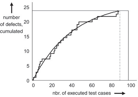
The test manager in the VSR project tracks the progress of the defect detection rate to control the test intensity of the different components. For better visibility, test effort was put on the x-axis and the cumulated number of detected failures was put on the y-axis. Figure 11-8 shows a stable if not slightly rising defect rate during testing (i.e., failure occurrence); in this case, it makes sense to continue or even intensify the test effort. However, figure 11-9 indicates saturation over time, which is a possible indicator to reduce the effort for this component.

Figure 11–8 Component A: stable defect detection percentage

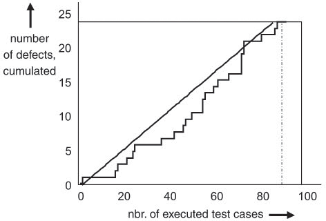
Figure 11–9 Component B: decreasing defect detection percentage

---

Defect-based metrics can also be used for trend analyses and predictions to make quantitative statements about defects still to be found during testing and defects that will remain after testing is completed. Such calculations, mostly based on statistical models, can be used for accompanying test control (see [Grottke 01], see also section 11.6).

Several more defect-based metrics are available:

Number of defects relative to test intensity (defect trend)

Number of defects relative to criticality (defect severity)

Number of defects per status (defect correction progress)

and so on

As time goes on, such metrics allow test management to make increasingly objective statements about the defect density expected in the system under development. Here and in many other test metrics, detected defects are classified and weighted prior to evaluation. IEEE Standard 1044 defines the defect classes and weights shown in table 11-3.

Table 11–3 Defect classes and weights

Defect class	Weight
Fatal	8
Severe	4
Medium	2
Minor	1
Nice to have	0.5

Further interesting indirect defect-based metrics can be created, for instance, by putting defect detection rates of different test levels in relation to each other.

The “defect removal leverage” (DRL), for example, is calculated as follows:

DRL = defect rate in test level X / defect rate in subsequent test level

In [Graham 00], we find a description of the “defect detection percentage” (DDP) metric, dividing all defects found at one test level by the sum of defects found at this and all subsequent test levels and in operation:

DDP metric

DDP = defects at test level X / defects at X and subsequent test levels (including operation)

If, for example, 40 defects were found in component testing, 19 in integration test, 30 in system test, 9 in acceptance test, and another 20 in production, the component test DDP is calculated as

40 / (40 + 19 + 30 + 9 + 20) = 40 / 118 = 0,339

that is, approximately 34%.

For integration test, DDP is calculated as

19 / (19 + 30 + 9 + 20) = 19 / 78 = 0,244

that is, approximately 24%.

For system testing, the DDP is

30 / (30 + 9 + 20) = 30 / 59 = 0,508

that is, approx. 50%.

In this case, effort could be shifted from system test to component and integration test. To be able to truly justify such shifts, the DDP is to be seen in relation to the effort planned for each test level.

Although defect-based test metrics are very important, care should be taken not to evaluate product quality solely on the basis of these metrics. If at some stage, test can only detect few or no defects at all, it depends on the quality of the test cases or the test process whether we are in a position to say that we have good product quality.

Caution: Do not use only defect-based metrics!

In order to get clear about the actual status of the “test quality” regarding particular functions, the “test design verification” metric puts quality (i.e., the number of detected defects) in relation to the quantity or test intensity (i.e., the number of test cases specified for and executed on a function). In addition, information is needed about the complexity or functional volume of the tested functions. Metrics underlying this metric are the number of test cases for a function and the number of failures detected by them, as well as a complexity measure appropriate to the test level—e.g., at the program text (in component testing) or requirements level (in system test).

Test design verification” metric

The “test design verification” metric provides some answers to the following questions:

Which functions show a high and which show a low number of failures?

What is the effort needed? That is, what is the number of required test cases needed to detect the defects?

Have the “right” (i.e., efficient) test cases been specified?

The following example explains the application of this metric.

---

Example: Test design verification chart

Figure 11-10 illustrates the graphical representation of the test design verification in form of a bubble diagram. For each function, the number of associated test cases is put on the x-axis, whereas the number of found failures is put on the y-axis.

The size of the bubbles represents the complexity of the respective function. We may expect in this kind of presentation to see the bubbles align on a straight line in the order of their size, because the more complex a function is

the more test cases are needed to test them, and

the more failures will occur during test execution.

Figure 11–10 Test design verification

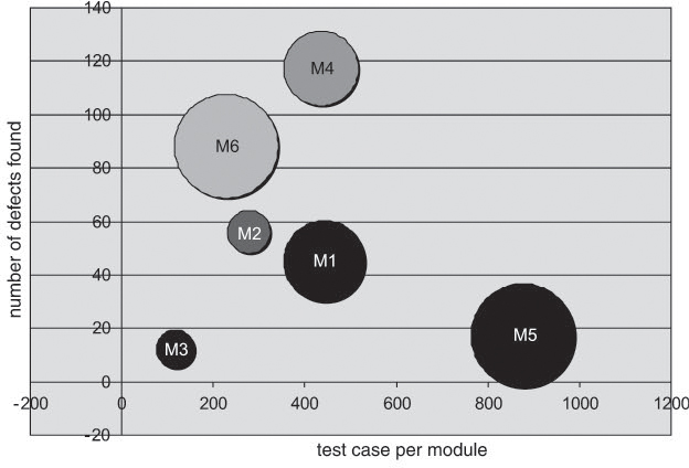
If a bubble is in the lower-right quadrant of the diagram, it means that the corresponding function has a large number of test cases assigned to it. These, however, find few failures. If the bubble is large, defect density is low and one may conclude that the function is obviously stable (see the M5 bubble in the example). If the bubble is small, it may be inferred that test design is inadequate in this area (“overengineering” of test cases).

If a bubble is in the top-left quadrant, the function has only a few test cases assigned to it; these, however, find many defects. Consequently, the defect density is high and the function is obviously unstable.

If we have a large bubble in the bottom-left quadrant (i.e., a small number of test cases and low defect detection), test cases are underengineered; i.e., test coverage of this function is low.

---

To track the defect rate, all detected failures must be reported during test execution. This requires an incident management system in which all reports and (status) changes are stored and historicized; i.e., they are time-stamped. Test completion, for instance, may be reached if the defect rate remains at a very low level over a certain period of time. This is an indication that test efficiency has been exhausted and that further effort spent on additional tests that will hardly find further failures may not be justified.

Keep track of progress!

The defect rate should be tracked separately for the different test levels, and ideally also for the different test techniques being used. The length of time that an actual defect rate stays below the maximum defect rate level and the required difference to the maximum defect rate are very sensitive values for the definition of test completion. A lot of experience and a sure instinct are needed for accurate targeting of theses values.

---

Example: Progression of the defect rate in the VSR system test

Studying the (typical) progression of the defect rate in the VSR system test, as shown in figure 11-11, the test manager notices that the defect rate bottoms out in weeks 6 to 9 only to show (as is often the case in practice) an upswing again in weeks 10 to 11. The first defect rate maximum is exceeded after most of the easily detected defects are found, whereas the renewed upturn marks the point where the more-difficult-to-find defects are uncovered. This rise, for instance, may have been caused by the test team’s better orientation toward the application to be tested.

Figure 11–11 Typical defect rate progression in system test

Figure 11–12 Defect report status

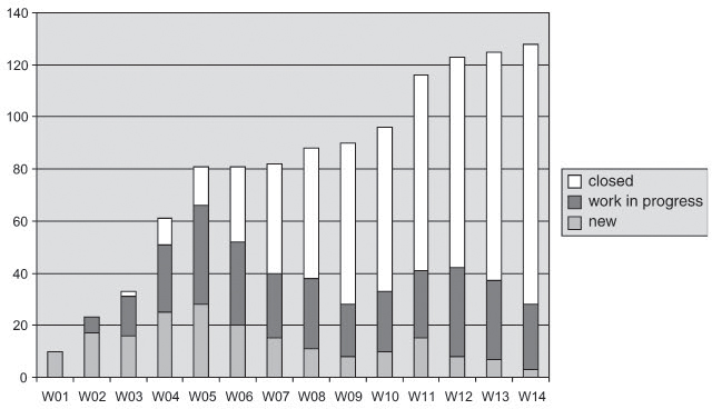
A look at the proportion of defect reports with status open (new), in progress, and closed shows that only very small software changes are to be expected as a result of further defect corrections. The test manager decides to continue testing for another week and then to break it off if the defect rate gets any lower.

---

To allow statistical projections regarding defect rates and residual defect probability, the data must be historicized in the incident database.

---

---

Example: Defect rate progression in the VSR system test

One hundred thirty-seven incidents were reported within one month of VSR acceptance testing, with 39 of them rated as class-1 defects. Out of the total of 524 incident reports held in the incident database at that time, 30% are change requests. Hence, the proportion of “genuine” defect reports is approximately 70%. Three hundred fifty-seven of the reports were written during integration test (internally reported failures), which corresponds to about 68% of the total reports. One hundred sixty-seven incident reports (i.e., 32%) come out of system and acceptance testing (externally reported failures).

Taking a code size of 100,284 new or changed lines and a number of 70% of 524 = 367 “genuine” incident reports, we get a defect density of 3.66 defects per 1,000 lines.

We may estimate the total number of defects in a newly implemented program to be at around 10 to 50 defects per 1,000 instructions; i.e., every 20th to 100th instruction is defective (see also [Hatton 97]). This rough estimate correlates with experiences made with spelling mistakes in newly written texts, and there is no reason to expect that fewer mistakes are made in coding (see also [Ebert 05]). However, at least half of all the defects injected during implementation should be found by the developers themselves during component testing.

New lines of code: Approximately 1-5 defects per 100 instructions!

The remaining 5 to 25 defects per 1,000 instructions should be found at the higher test levels. All in all, the defect rate is below average and testing has to be intensified.

---

11.5.4 Cost- and Effort-Based Metrics

Effort-based metrics provide the context for financial and time-related measurements and can, once they have been collected in some projects, be used in the planning of future test projects. Here are some examples:

Number of person days for test planning or specification

Number of person days for the creation of test procedures

Number of person days per detected defect

Number of person hours per defect removal

Measurement values of that kind are to be anonymized and reported to project members in the form of feedback, including mean values.³ Interpreting values, we must always bear in mind that besides specifying, executing, and documenting test cases, testers require additional time for the planning of their own tests as well as for setting up the test environment and checking in and out version-dependent test cases, etc.

Make metrics anonymous.

In the end, the most important success criterion is that during the introduction of a measurement program, everybody involved or impacted fully understands the purpose of data collection.

11.5.5 Evaluating Test Effectiveness

Software tests are effective if they find defects and increase confidence in the software. To assess test effectiveness, defect rate, test coverage, and test effort are taken into account.

Testing means detecting defects and providing confidence.

In order to calculate the degree of defect detection (DDD), the weighted defect or failure ratio (see the example in table 11-3) detected during test is divided by the total number of detected defects or failures. Thus, we get

DDD = number of weighted defects in test / total number of defects found

Confidence in a system grows in proportion to the used measure (e.g., system use time, CPU time, etc.) if no failures occur. For test, system use is primarily understood to be the number of already executed test cases, and confidence in the system decreases in the same proportion as the number of detected failures increases.

The basic idea behind the following metric is that the defect rate states only the number of weighted defects per test case but does not say anything about the software part that is covered or not covered by test. Let us assume that the first test cycle has detected 0.05 weighted defects per test case and a later cycle with exactly the same test cases comes up with only 0.01 weighted defects per test case. Is this an indication that our confidence in the system can rise by 500%? Of course not, because we can have confidence only in what has truly been tested. Hence, we have to see defect rate relative to the degree of test coverage. The confidence level (CL) is calculated as

CL = 1 – (number of weighted defects/number of executed test cases) × degree of test coverage

Finally, test effectiveness (TE) is the product of the two metrics, degree of defect detection and confidence level:

TE = DDD × CL

Tom DeMarco recommends collecting the following eight metrics for each version of a software product to obtain information about the (financial) effectiveness of the test processes ([DeMarco 86]):

DeMarco’s metrics on test effectiveness

Detected project faults: number of defects found and corrected prior to delivery of the product

Project fault density: detected project defects/KDSI

Project damage: defect correction costs prior to delivery in $/KDSI

Delivered faults: Number of defects found after product delivery

Product fault density: delivered defects/KDSI

Product damage: defect correction costs after delivery in $/KDSI

Total damage: project damage + product damage

Product damage at six months: defect correction costs in the first six months after delivery in $/KDSI

In this connection, it is necessary to use the actual accrued overall diagnosis and repair costs and not merely the defect detection costs. The test process is effective if test costs do not exceed the overall cost of damage.

11.6 Residual Defect Estimations and Reliability

Based on available data about the product and the development and test processes, the techniques described in this section will enable us to use statistical means to make statements about the expected system reliability, which can be estimated based on the residual defects in the system after test completion. In particular, these statements serve as indicators for the product risk (see chapter 9). Principally, this can be done as follows:

Experience-based estimation of the residual defect probability

Statistical analysis of the defect data and reliability growth model

Both experience-based estimation of the residual defect probability and defect data analysis require that test cases adequately reflect the operational profile (see also [Voas 00]); i.e., the expected distribution of the use frequency of the product functions during operation. Considering the test techniques described in Software Testing Foundations on the specification of methodical tests, this only holds true for business-process-based tests. In order to apply the techniques for residual defect estimation described on the following pages, one usually needs to define additional test cases that complement the existing system tests with regard to the operational profile.

Identify the operational profile for reliability analysis.

11.6.1 Residual Defect Probability

There are basically three possibilities to evaluate the test process based on the observed number of detected defects:

Estimate the number of defects inherent in the system prior to test and estimate the number of defects to be found.

Monitor the defect detection percentage.

Inject artificial failures into the program code of which a certain proportion is to be found during testing.

To be able to work with estimated target defect numbers, you must estimate the total number of all system inherent failures. Since these are failures that have remained in the system after code reviews or other quality assurance measures, this process is also called → residual defect estimation.

These estimations are based on data and experience values present in a particular development unit and especially in a well-managed incident database. Subsequently, the effectiveness of future tests is estimated for each test level (as a percentage of the detected defects). Based on these estimations, the number of defects still to be found can be calculated as follows:

target number of defects = residual number of defects × effectiveness (in %)

From this we can see that the effectiveness estimation in fact corresponds with the target number of failures expected to be detected by test.

---

Example

The following sample calculation explains the estimation of defects found by test (effectiveness estimation), which is done based on targets set in table 11-4.

Table 11–4 Test effectiveness targets

Test level	Found coding errors	Found design errors
Component testing	65%	0%
Integration testing	30%	60%
System testing	3%	35%
Sum	98%	95%

All in all, about 98% of all coding errors and 95% of design errors are supposed to be detected during test. These defects have remained in the system despite all the other quality assurance activities.

A number of 5 defects per 100 instructions is assumed as an estimation of the residual defects in a system with more than 10,000 instructions. Thus, a system with approximately 10,000 instructions has a residual defect rate of approximately 500 defects.

As a target for the number of defects still to be found, we also assume that the ratio of coding or design errors among the residual defects is 2:3; i.e., out of the approximately 500 residual defects we get 200 coding and 300 design errors.

Using the above formula, the defect targets for columns “Target coding errors” and “Target design errors” can now be calculated quite easily (table 11-5).

Table 11–5 Calculated defect targets for code and design errors

Test level	Defect target (total)	Target coding errors	Target design errors
Component testing	130	130	0
Integration testing	240	60	180
System testing	111	6	105
Sum	481	196	285

These targets can be used as a test completion criterion with regard to coding and design errors if the detected failures have been classified accordingly. The total defect target is the sum of defects to be found at the respective test level.

11.6.2 Reliability Growth Model

The statistical software reliability calculation tries to make statements about future abnormal software behavior based on existing defect data (times of detection of a failure or defect) of defects found primarily in integration and system test. This may be the number or rate of future expected failures or the supposed number of defects still resident in the software.

Infer reliability from defect data.

Here we need to consider that because statistical software reliability calculations are based on the theory of probability, the quality of prediction will rise with the amount of data that can be used for calculation and with the size of the project and organization. The larger the database, the less impact “outliers” have. Moreover, the earliest time from which we should consider defect data is the beginning of integration test, since in component testing we can not expect representative use of the software. There, only certain individual aspects of the software are tested and tests do certainly not reflect the system’s operational profile.

This section describes two software reliability calculation models and provides some directions concerning the preconditions and application of such models. Basic conditions that must be adequately satisfied before using the statistical software reliability calculation models are as follows:

Software development and test processes are stable; i.e., the software is developed (further) and tested by well-trained engineers following a defined development model with recognized methods and known tools.

Statistics only work if the context is stable.

Test cases and test data reflect the operational conditions of software in production sufficiently well (test profile corresponds to operational profile). Some models, however, are also suitable for predictions in the area of systematic, structured testing (see [Grottke 01]).

Gross simplification

Test cases cover all defects in a particular defect class with the same probability.

Failures can be clearly mapped to defects.

The Jelinski-Moranda model ([Jelinski 72], see also [Lyu 96]) is described as a simple model and based on some further, simplifying preconditions in addition to the ones just mentioned:

The defect rate is in proportion to the total number of defects residing in the software.

The interval between the occurrence of every two defects is constant (constant test intensity).

During fault correction no new defects are injected into the software.

The first supposition concomitantly implies the model’s basic idea: The current defect rate is used to deduce the total number of defects. Take N₀ to be the total number of failures prior to testing, p a constant of proportionality, and λ₀ the defect rate at the beginning of test.

The basic idea of the model is expressed as

λ₀ = p × N₀

At a later point in time i, after N₀ – N_i defects have been corrected, we have

λ_i = p × N_i

Here, N_i constitutes all the failures still residing in the software at the time i. The probability that the software will function without failure for a specific period of time (→survival probability) is calculated as follows (see [Liggesmeyer 02]):

R(t) = e^{-λi · t}

---

Example: VSR system reliability

At the beginning of VSR integration testing, a new failure is detected every 1.25 hours (operational or test execution time); at the end of system test, a new failures is detected only every 20 hours. The test team detected 725 failures in these tests and removed them. The test manager calculates the following equations:

λ₀ = p × (N₀ – 0) = 1 / 1.25 h = 0.8 / h

and

λ_End = p × (N₀ – 752) = 1 / 20 h = 0.05 / h,

i.e.,

λ₀/λ_End = 16

This equation is first solved to give

N₀ = 802

Inserting this value into the first equation gives

p = 0.001

He continues to calculate:

R(10h) = e^-0.05×10h = 0.6065

This means that the probability that the VSR software will function for 10 hours without failure is approximately 61%.

Since this does not seem acceptable to the project team, the test phase is extended. During the extension period, 25 more failures are detected, giving the following picture:

λ_n = 0.001 × (802 – 777) = 0.025 / h

This means that the test manager can expect further failures to be found only every 40 hours.

R (10 h) = e^-0.025×10h = 0.779

As a result of further testing, the system’s probability to last 10 hours without failure has increased by approximately 17%, thus directly quantifying the benefit of further testing.

---

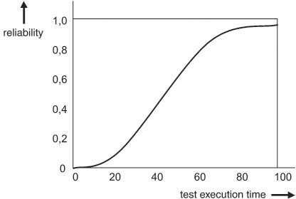
Another model worth looking at is the Musa-Okumoto model ([Musa 84]), which puts particular focus on the fact that at the beginning of the test phase we are more likely to detect the “simple” failures, as a result of which software reliability will only grow slowly. Instead of the inverse-exponential increase of the probability of survival, we get an S-shaped progression.

Figure 11-13 shows the progression of N(t) for a (normalized) number of defects N₀ = 1, β = 0.05 × 1 / h and 100 hours of test execution time.

Figure 11–13 Reliability growth in the Musa-Okumoto model

Many more reliability estimation models can be found in the literature; a general overview is given in [Liggesmeyer 02] (in German), and the standard reference regarding software reliability is still [Lyu 96].

11.7 Summary

For each test level, suitable test metrics need to be defined and collected. Test metrics allow quantitative statements regarding product quality and the quality of the development and test processes and form the basis for transparent, reproducible, and traceable test process planning and control.

Based on the measurement objects, we get test-case-based metrics, test-basis- and test-object-based metrics, defect-based metrics, and and cost- and effort-based metrics.

Complexity metrics such as lines of code (LOC) and cyclomatic complexity (McCabe metric) are required for risk-based testing. Test metrics, too, serve as indicators for project and product risks.

Historicized incident data allows for defect-based metrics as well as statements regarding residual defect probability and system reliability.