
Chapter 4
Statistical Learning
Arthur Charpentier
Université du Québec á Montrél
Montréal, Québec, Canada,
Stéphane Tufféry
ENSAI & Université de Rennes 1
Rennes, France
4.1 Introduction and Motivation
In this chapter, we will describe some techniques to learn from data, and to make a prediction based on a set of features. We will use a training set, where those features were observed, as well as our variable of interest, to build a predictive model. A good model will accurately predict the variable of interest. This is actually a standard procedure in actuarial science, where the variable of interest might be
- Whether an insured will buy additional (optional) coverage, or not
- Whether a claimant will be represented by an attorney, or not (see e.g. the automobile injury insurance claims in Frees (2009))
- Whether an insured will have some specific disease, or not
- Whether a loaner will be considered a good or a bad client (in this chapter)
All the techniques mentioned in this chapter will be used on a binary variable of interest (good or bad client), but one can easily extend most of them to an ordered discrete variable of interest.
4.1.1 The Dataset
The dataset is consumer credit files, called the German Credit dataset in Tufféry (2011) and Nisbet et al. (2011), with 1,000 instances, that can be found in the CASdataset package, under the name credit. New applicants for credit and loans can be evaluated using twenty explanatory variables:
- Att. 1 (qualitative) checking_status, status of existing checking account, A11 : less than 0 euro, A12 : from 0 to 200 euros, A13 : more than 200 euros, and A14 : no checking account (or unknown).
- Att. 2 (numeric) duration, credit duration in months.
- Att. 3 (qualitative) credit_history, credit history A30 : delay in paying off in the past, A31 : critical account, A32 : no credits taken or all credits paid back duly, A33 : existing credits paid back duly till now, A34 : all credits at this bank paid back duly.
- Att. 4 (qualitative) purpose, purpose of credit, A40 : car (new), A41 : car (used), A42 : furniture/equipment, A43 : radio/television, A44 : domestic appliances, A45 : repairs, A46 : education, A47 : (vacation—does not exist in the study sample), A48 : retraining, A49 : business, A410 : others.
- Att. 5 (numerical) credit_amount, credit amount
- Att. 6 (qualitative) savings, savings account A61 : less than 100 euros, A62 : from 100 to 500 euros, A63 : from 500 to 1,000, A64 : more than 1,000, A65 : no savings account (or unknown).
- Att. 7 (qualitative) employment, Present employment since, A71 : unemployed, A72 : less than 1 year, A73 : from 1 to 4 years, A74 : from 4 to 7 years, A75 : more than 7 years.
- Att. 8 (numerical) installment_rate, Installment rate (in percentage of disposable income)
- Att. 9 (qualitative) personal_status, Personal status and sex, A91 : male : divorced/separated, A92 : female : divorced/separated/married, A93 : male : single, A94 : male : married/widowed, A95 : female : single.
- Att. 10 (qualitative) other_parties, Other debtors or guarantors, A101 : none, A102 : co-applicant, A103 : guarantor.
- Att. 11 (numerical) residence_since, Present residence since, 1 : < 1 year, 2 : < ... < 4 years, 3:4 < ... < 7 years, 4 : > 7 years
- Att. 12 (qualitative) property_magnitude, Property (most valuable) , A121 : real estate, A122 : if not A121 : building society savings agreement/life insurance, A123 : if not A121/A122 : car or other, not in attribute 6, A124 : unknown / no property.
- Att. 13 (numerical) age, Age (in years)
- Att. 14 (qualitative) other_payment_plans, Other installment plans, A141 : bank, A142 : stores, A143 : none.
- Att. 15 (qualitative) housing, Housing, A151 : rent, A152 : own, A153 : for free
- Att. 16 (numerical) existing_credits, Number of existing credits at this bank (including the running one)
- Att. 17 (qualitative) job, Job, A171 : unemployed/ unskilled - non-resident, A172 : unskilled - resident, A173 : skilled employee / official, A174 : management/ selfemployed/highly qualified employee/officer.
- Att. 18 (numerical) num_dependents, Number of people being liable to provide maintenance for.
- Att. 19 (qualitative) telephone, Telephone, A191 : none, A192 : yes, registered under the customers name.
- Att. 20 (qualitative) foreign_worker, foreign worker, A201 : yes, A202 : no.
We will remove the latter variable in the study.
> credit <- credit[,-which(myVariableNames == "foreign_worker")]
In the previous description, variables are characterized as either quantitative (numerical) or qualitative (called factors in the first chapter).
In this chapter, we will see how to develop a credit scoring rule that can be used to determine if a new applicant is more likely to be either a good credit risk, or a bad credit risk, based on values for one, or more, of the explanatory variables:
- Att. 21 (qualitative) class, binary variable 0 stands for good and 1 bad (or creditworthy against not credit-worthy, or no non-payments against existing nonpayments)
In order to have a 0/1 variable, use
> credit$class <- credit$class-1
> table(credit$class)
0 1
700 300
This dataset can be found in library caret using data(GermanCredit) (see Kuhn (2008)).
4.1.2 Description of the Data
Most of the variates are factor variables. It is also possible to cut continuous variates to define factor ones:
> credit.f <- credit
> credit.f$age <- cut(credit.f$age,c(0,25,Inf))
> credit.f$credit_amount <- cut(credit.f$credit_amount,c(0,4000,Inf))
> credit.f$duration <- cut(credit.f$duration,c(0,15,36,Inf))
A natural tool to quantify correlation between categorical variates is Cramer's V (from Cramer (1946)), defined as
where X2 is the statistics associated to Pearson's chi-squared test of independence, n is the number of observations, and k denotes the number of factors, for the two variates, whichever is less (here, k — 1 will always be 1 because the variable of interest takes only two values).
> library(rgrs)
> k <- ncol(credit.f)-1
> cramer = function(i) cramer.v(table(credit.f[,i],credit.f$class))
It is also possible to use
> cramer = function(i) sqrt(chisq.test(
+ table(credit.f[,i],credit.f$class))$statistic/(length(credit.f[,i])))
Then,
> pv <- function(i) chisq.test(table(credit.f[,i],credit.f$class))$p.value
> CRAMER <- data.frame(variable=names(credit)[1:k],
> cramerv <- Vectorize(cramer)(1:k),
> p.value <- Vectorize(pv)(1:k))
> vCRAMER <- CRAMER[order(CRAMER[,2], decreasing=TRUE),]
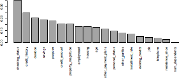
It is possible to plot the variates, sorted by correlation level:
> par(mar=c(10,4,4,0))
> barplot(vCRAMER[,2],names.arg=vCRAMER[,1],las=3)
For continuous variates X (and categorical variable Y), it is possible to compare the conditional distribution of X given Y:
> aggregate(credit[,c("age","duration")],by=list(class="credit$class),mean)
class Group.1 age duration
1 0 36.22429 19.20714
2 1 33.96333 24.86000
It is possible also to visualize the probability that Y = 1 for some value x of X, or for some partition of the X variable,
> Q <- quantile(credit$age,seq(0,1,by=.1))
> Q[1] <- Q[1]-1
> cut.age <- cut(credit$age,Q)
> (prop <- prop.table(table(cut.age,credit$class),1))
cut.age 1 2
(18,23] 0.6000000 0.4000000
(23,26] 0.6148148 0.3851852
(26,28] 0.7021277 0.2978723
(28,30] 0.6623377 0.3376623
(30,33] 0.6857143 0.3142857
(33,36] 0.7927928 0.2072072
(36,39] 0.7567568 0.2432432
(39,45] 0.7256637 0.2743363
(45,52] 0.8000000 0.2000000
(52,75] 0.6979167 0.3020833
that can be visualized (Figure 4.2) using
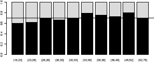
> barplot(t(prop))
> abline(h=mean(credit$class="=0),lty=2)
4.1.3 Scoring Tools
The variable of interest here is a 0/1 variate Y. The goal here is to use explanatory variables X to predict Y, based on a continuous score function (as introduced by Fisher (1940)). The prediction will then be
for some threshold . From a decision theory perspective, it will be interesting to compare the true value, and the predicted one, as in Table 4.1.
Decision and errors in credit scoring.
True value of Y |
|||
Y=0 |
Y=1 |
||
(negative) |
(positive) |
||
Y = 0 |
(negative) |
Correct decision |
Type II error |
Y = 1 |
(positive) |
Type I error |
Correct decision |
Type I errors are also called false positive, while type II error are false negative. In a perfect world, we would like those two errors to be as small as possible. The choice of the threshold will be used to make a tradeoff between the two kinds of errors, but we will have to spend some time to have both errors as small as possible.
A standard tool to visualize the fit is the ROC curve (Receiver operating characteristic, From communication theory) created by plotting the fraction of true positives out of the positives (the true positive rate) versus the fraction of false positives out of the negatives (false positive rate), at various threshold settings. Consider a simple latent-based model, where we assume that Y = 1 when some credit indicator (unobservable) Y* is too high, where Y* is assumed to be continuous and a function of some covariates. With a linear model, , where ε is a centered Gaussian noise. Thus, here
This is the so-called probit model. The code to construct the score function is
> Y <- credit$class
> reg <- glm(class~age+duration,data=credit,family=binomial(link="probit"))
> summary(reg)
Call:
glm(formula = class ~ age + duration, family = binomial(link = "probit"),
   data = credit)
Deviance Residuals:
Min 1Q Median 3Q Max
-1.5364 -0.8400 -0.7084 1.2452 2.1074
Coefficients:
Estimate Std. Error z value Pr(>|z|)
(Intercept) -0.645078 0.161121 -4.004 6.24e-05 ***
age -0.010685 0.003888 -2.748 0.00599 **
duration 0.022887 0.003467 6.602 4.05e-11 ***
---
Signif. codes: 0 *** 0.001 ** 0.01 * 0.05 . 0.1 1
(Dispersion parameter for binomial family taken to be 1)
Null deviance: 1221.7 on 999 degrees of freedom
Residual deviance: 1169.0 on 997 degrees of freedom
AIC: 1175
Number of Fisher Scoring iterations: 4
> S <- pnorm(predict(reg))
For that score, it is possible to plot the ROC curve using
> FP <- function(s) sum((S>s)*(Y==0))/sum(Y==0)*100
> TP <- function(s) sum((S>s)*(Y==1))/sum(Y==1)*100
> u <- seq(0,1,length=251)
> plot(Vectorize(FP)(u),Vectorize(TP)(u),type="s",
+ xlab="False Positive Rate (%)",ylab="True Positive Rate (%)")
> abline(a=0,b=1,col="grey")
This function can be obtained using functions performance and prediction from the library(ROCR):
> library(ROCR)
> pred <- prediction(S,Y)
> perf <- performance(pred,"tpr", "fpr")
> plot(perf)
It is also possible to plot confidence bands, using either library(verification) or library(pROC):
> library(verification)
> roc.plot(Y,S, xlab = "False Positive Rate",
+ ylab = "True Positive Rate", main = "", CI = TRUE,
+ n.boot = 100, plot = "both", binormal = TRUE)
> library(pROC)
> roc <- plot.roc(Y,S,main="", percent=TRUE, ci=TRUE)
> roc.se <- ci.se(roc,specificities=seq(0, 100, 5))
> plot(roc.se, type="shape", col="grey")
Those four graphs can be visualized on Figure 4.3.
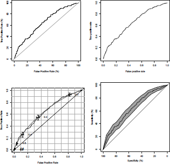
ROC curve (true positive rate versus false positive rate) from a probit model on the age and the duration of the loan, using our own codes, ROCR, verification and pROC packages.
The performance curve of the scoring function S is the graph , where
The selection curve of the scoring function S is the function
.
Practitioners also use those functionals to derive indicators (see Hand (2005) for a discussion). According to May (2004), Kolmogorov-Smirnov statistics (called the K-S statistic) “is the most widely used statistic within the United States for measuring the predictive power of rating systems,” but “this does not seem to be the case in other environments, where the Gini seem to be more prevalent” (see also Anderson (2007)). The code to compute the K-S statistic, using outputs from the ROCR package, is
> max(attr(perf,'y.values')[[1]]-attr(perf,'x.values')[[1]])
[1] 0.1966667
which is the largest difference between the cumulative true positive and cumulative false positive rate. This statistic can be visualized on Figure 4.4.
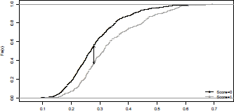
> plot(ecdf(S[credit$class="=0]),main="",xlab="", pch=19,cex=.2)
> plot(ecdf(S[credit$class="=1]),, pch=19,cex=.2, col="grey",add=TRUE)
> legend("bottomright",c("Score=0","Score=1"), pch=19,col=c("black","grey"),lwd=1,bty="n")
> perf <- performance(pred,"tpr", "fpr")
> ks <- [email protected][[1]][email protected][[1]]
> (seuil <- pred@cutoffs[[1]][which.max(ks)])
827
0.279034
> arrows(seuil,[email protected][[1]][which.max(ks)],seuil,
+ [email protected][[1]][which.max(ks)],col=,black',length = 0.1,code=3)
The AUC (area under the ROC curve) statistic is another way to measure predictive power of models, and the code is
> performance(pred,"auc")
Note that here we obtain 0.6405:
Slot "y.values":
[[1]]
[1] 0.6405286
This area is included between 0 and 1, and the more it is close to 1, the more predictive is the model. In that case, the ROC curve will hug the top left corner (indicating a high true positive rate and a low false positive rate).
4.1.4 Recoding the Variables
There is here a large number of factors, and all of them have a large number of modalities. Using the recode function, it is possible to recode the variables, and to merge modalities.
> library(car)
> credit.rcd <- credit.f
> credit.rcd$checking_status <- recode(credit.rcd$checking_status,
"'A14'='No checking account';'A11'='CA < 0 euros';'A12'=
+ 'CA in [0-200 euros[';'A13'='CA > 200 euros' ")
> credit.rcd$credit_history <- recode(
+ credit.rcd$credit_history,
+ "c('A30','A31')= 'critical account';
+ c('A32','A33')='existing credits paid back duly till now';
+ 'A34'='all credits paid back duly'")
> credit.rcd$purpose <- recode(
+ credit.rcd$purpose,"'A40'='Car (new)';
+ 'A41'='Car (used)';c('A42','A43','A44','A45')='Domestic equipment';c('A46','A48'
+ ,'A49')='Studies-Business';
+ 'A47'='Holidays';else='Else'")
> credit.rcd$savings <- recode(credit.rcd$savings,"c('A65','A63','A64')=
+ 'No savings or > 500 euros';c('A62','A61')='< 500 euros'")
> credit.rcd$employment <-
+ recode(credit.rcd$employment,"c('A71','A72')='unemployed or < 1 year';'A73'=
+ 'E [1-4[years';c('A74','A75')='> 4 years'")
> credit.rcd$personal_status <-
+ recode(credit.rcd$personal_status ,
+ "'A91'=' male divorced/separated';'A92'='female divorced/separated/married';
+ c('A93','A94')='male single/married/widowed';'A95'='female : single'")
> credit.rcd$other_parties <- recode(credit.rcd$other_parties,"'A103'='guarantor';else='none'")
> credit.rcd$property_magnitude <-
+ recode(credit.rcd$property_magnitude,"'A121'='Real estate';'A124'='No property';
+ else='Else'")
> credit.rcd$other_payment_plans <-
+ recode(credit.rcd$other_payment_plans,"'A143'='None';else='Banks-Stores'")
> credit.rcd$housing <-
+ recode(credit.rcd$housing,"'A152'='Owner';else='Else'")
Using those labels will help in the interpretation of our models.
4.1.5 Training and Testing Samples
The natural technique to generate a sub-sample is to use the sample function:
> set.seed(123)
> index <- sort(sample(nrow(credit), 644, replace=FALSE))
> table(credit$class[index])
1 2
447 197
In order to reproduce some outputs obtained in Tufféry (2011), using SAS®, we have to use another random number generator, based on Fishman & Moore (1982):
> library(randtoolbox)
> set.generator(name="congruRand", mod=2~(31)-1,mult=397204094, incr=0, seed=123)
> U=runif(1000)
> index <- sort(which(rank(U)<=644))
> table(credit$class[index])
0 1
451 193
The training sample will be based on the 644 observations, and the remaining 356 will be used as the validation sample:
> train.db <- credit.rcd[index,]
> valid.db <- credit.rcd[-index,]
4.2 Logistic Regression
The first model that we will consider is logistic regression (see Hosmer & Lemeshow (2000) or Hilbe (2009)). As mentioned in Thomas (2000), logistic regression is now the most widely used method in credit scoring.
From a computational point of view, logistic regression is a Generalized Linear Model where the distribution of the endogenous variate is binary. Thus, in R, the code to run a logistic regression is
> reg <- glm(Y~X1+X2+X3,data=df,family=binomial(link='logit'))
4.2.1 Inference in the Logistic Model
Let Yi denote random variables taking values , with probability and (respectively), that is,
with Here while
If we assume that are identical (denoted ) and Y are independent, then—see Chapter 2— π can be estimated using maximum likelihood techniques. Here, the likelihood is
and the log-likelihood becomes
The first-order condition is
Assume now that are different, and a function of some covariates, , so that . To be more specific, using the standard matrix notation,
> Y <- credit[index,"class"]> X <- as.matrix(cbind(1,credit[index,c("age","duration")]))
A linear model, will not be suitable, because can be negative, or larger than 1. Parametrization with the probability yields too many constraints, so a natural idea is to model the odds, or the logarithm of the odds ratio:
or equivalently,
In that case, the log-likelihood becomes
The gradient is
since, from the expression of
Because there is no analyticaslolution for this expression, it is natural to use Newton- Raphson's algorithm:
- Start from some initial value
- Set
a loop, where is the gradient of the log-likelihood, and H(β) the Hessian matrix, with generic term
Here,
and We do recognize a weighted regression, with weights Ω.
Our starting points can be estimators from a standard linear regression:
> beta <- as.vector(lm(Y~0+X[,1]+X[,2]+X[,3])$coefficients)
> BETA <- NULL
> for(s in 1:6){
+ pi <- exp(X%*%)/(1+exp(X%*%beta))
+ gradient <- t(X)%*%(Y-pi)
+ omega <- matrix(0,nrow(X),nrow(X));diag(omega)=(pi*(1-pi))
+ hessian <- -t(X)%*%omega%*%X
+ beta <- beta-solve(hessian)%*%gradient
+ BETA <- cbind(BETA,beta)
+}
Observe that, actually, four iterations would be sufficient:
> BETA
[,1] [,2] [,3] [,4] [,5] [,6]
1 -1.08304581 -1.10983815 -1.10665019 -1.10663432 -1.10663432 -1.10663432
age -0.01281867 -0.01754473 -0.01786453 -0.01786550 -0.01786550 -0.01786550
duration 0.03395857 0.03968785 0.03991297 0.03991347 0.03991347 0.03991347
Under mild regularity conditions
where I(β) = —H(β), thus the asymptotic variance-covariance matrix is hessian:
> (SD <- sqrt(diag(solve(-hessian))))
1 age duration
0.342223292 0.008673299 0.007171971
A coefficient is said to be significant if the p-value associated to the Student test is smaller than 5%. That p-value is computed as follows:
> cbind(BETA[,6],SD,BETA[,6]/SD,2*(1-pnorm(abs(BETA[,6]/SD))))
SD
1 -1.10663432 0.342223292 -3.233662 1.222142e-03
age -0.01786550 0.008673299 -2.059828 3.941499e-02
duration 0.03991347 0.007171971 5.565202 2.618487e-08
Those values can be obtained using summary of a glm object:
> reg <- glm(class~age+duration,data=credit[index,],
+ family=binomial(link="logit"))
> summary(reg)
Call:
glm(formula = class ~ age + duration, family = binomial(link = "logit"),
data = credit[index,])
Deviance Residuals:
Min 1Q Median 3Q Max
-1.5814 -0.8382 -0.7007 1.2380 2.0974
Coefficients:
Estimate Std. Error z value Pr(>|z|)
(Intercept) -1.106634 0.342223 -3.234 0.00122 **
age -0.017866 0.008673 -2.060 0.03941 *
duration 0.039913 0.007172 5.565 2.62e-08 ***
---
Signif. codes: 0 *** 0.001 ** 0.01 * 0.05 . 0.1 1
(Dispersion parameter for binomial family taken to be 1)
Null deviance: 786.45 on 643 degrees of freedom
Residual deviance: 750.43 on 641 degrees of freedom
AIC: 756.43
Number of Fisher Scoring iterations: 4
We do recognize the estimators and their standard errors obtained above (with only four iterations).
4.2.2 Logistic Regression on Categorical Variates
Consider, first, a model with one categorical regressor, for instance credit_history, with five modalities in the original credit database:
> reg <- glm(class~credit_history,data=credit,family=binomial(link="logit"))
> summary(reg)
Call:
glm(formula = class ~ credit_history, family = binomial(link = "logit"),
 data = credit)
Deviance Residuals:
Min 1Q Median 3Q Max
-1.4006 -0.8764 -0.6117 1.0579 1.8805
Coefficients:
Estimate Std. Error z value Pr(>|z|)
(Intercept) 0.5108 0.3266 1.564 0.117799
credit_historyA31 -0.2231 0.4359 -0.512 0.608703
credit_historyA32 -1.2698 0.3396 -3.739 0.000185 ***
credit_historyA33 -1.2730 0.3988 -3.192 0.001413 **
credit_historyA34 -2.0919 0.3616 -5.784 7.28e-09 ***
---
(Dispersion parameter for binomial family taken to be 1)
Null deviance: 1221.7 on 999 degrees of freedom
Residual deviance: 1161.3 on 995 degrees of freedom
AIC: 1171.3
Number of Fisher Scoring iterations: 4
In that case, the value predicted per category is exactly the empirical one:
> cbind(prop.table(table(credit$credit_history,credit$class),1),
+ logit=predict(reg,newdata=data.frame(credit_history=
+ levels(credit$credit_history)), type="response"))
0 1 logit
A30 0.3750000 0.6250000 0.6250000
A31 0.4285714 0.5714286 0.5714286
A32 0.6811321 0.3188679 0.3188679
A33 0.6818182 0.3181818 0.3181818
A34 0.8293515 0.1706485 0.1706485
In the case of two categorical regressors, the interpretation is rather different. In the credit.rcd database (in order to have less modalities), consider the credit_history variable (three modalities) and the purpose variable (five modalities).
> reg <- glm(class~credit_history*purpose,data=credit.rcd,
+ family=binomial(link="logit"))
> p.class="matrix(predict(reg,newdata=data.frame(
+ credit_history=rep(levels(credit_history),each=length(levels(purpose))),
+ purpose=rep(levels(purpose),length(levels(credit_history)))),type="response"),
+ ncol=length(levels(credit_history)),
+ nrow=length(levels(purpose)))
> rownames(p.class) <- levels(purpose)
> colnames(p.class) <- levels(credit_history)
> p.class
all credits paid back duly critical account paid back duly
Car (new) 0.2435897 0.7368421 0.4087591
Car (used) 0.1111111 0.3750000 0.1694915
Domestic equipment 0.1313869 0.5161290 0.2996942
Else 0.3333333 0.9999995 0.1666667
Studies-Business 0.2051282 0.6071429 0.3595506
Here, a product of the two regressors was considered. But in the context of standard linear models, the prediction will not be equal to the empirical average value:
> reg <- lm(class~credit_history*purpose,data=credit.rcd)
> p.class.linear=matrix(predict(reg,newdata=data.frame(
+ credit_history=rep(levels(credit_history),each=length(levels(purpose))),
+ purpose=rep(levels(purpose),length(levels(credit_history)))),type="response"),
+ ncol=length(levels(credit_history)),
+ nrow=length(levels(purpose)))
> rownames(p.class.linear) <- levels(purpose)
> colnames(p.class.linear) <- levels(credit_history)
> p.class.linear
all credits paid back duly critical account paid back duly
Car (new) 0.23626428 0.6872147 0.4198125
Car (used) 0.08633173 0.4015839 0.1810066
Domestic equipment 0.14817277 0.5526530 0.2891990
Else 0.21699668 0.6631013 0.3932843
Studies-Business 0.19263547 0.6288823 0.3581855
If instead of modelling probabilities, we compute odds ratios,
> p.class.linear/(1-p.class.linear)
all credits paid back duly critical account paid back duly
Car (new) 0.30935346 2.197081 0.7235806
Car (used) 0.09448914 0.671078 0.2210110
Domestic equipment 0.17394698 1.235401 0.4068636
Else 0.27713380 1.968251 0.6482185
Studies-Business 0.23859789 1.694563 0.5580827
we observe that rows and columns, here, are proportionals, which is a consequence of the logistic regression, as odds ratios is a multiplicative model.
4.2.3 Step-by-Step Variable Selection
In stepwise selection, the choice of predictive variables is carried out by an automatic procedure, based on some specified criterion. As with the regression tree (and the CART algorithm), with a lot of covariates, the number of possible models can become too large extremely fast: with np covariates, there are 2np possible models. With twenty covariates, there will be more than a million models to compare. Two approaches are usually considered:
- ● A forward selection, which involves starting with no variables in the model. Then the addition of each variable is tested (based on the criterion considered); we then add the variable (if any) that improves the model the most, and repeat this process until none improves the model significantly.
- ● A backward selection, which involves starting with all variables in the model. Then the deletion of each variable is tested (based on the criterion considered); we then remove the variable (if any) that improves the model the most by removing, and repeat this process until none improves the model significantly.
The most common criteria are based on penalization of the log-likelihood. One might think of the adjusted R2 in the context of linear regression. For instance, if np denotes the number of parameters in the fitted model, — log L + k.np is the usual AIC (Akaike Information Criterion) when k = 2, while it is Schwarz's Bayesian Criterion (BIC) when k = log(n). The generic function to compute those values is
> AIC(model,k=2)
> AIC(model,k=log(nobs(model)))
for some fitted model. In the context of linear models, those criteria are equal (up to an additive constant) to n times the logarithm of the sum of squares of the residuals. For example, the AIC is
AIC = constant + n log(sum of squares of the residuals) + 2np.
Another popular criterion is Mallows' defined as
where is the estimated error variance for the largest model that can be considered. Again, this statistic adds a penalty to the (logarithm of the) sum of squares of the residuals. As earlier, the penalty increases as the number of predictors in the model increases. Interesting models should have a small .
4.2.3.1 Forward Algorithm
The procedure here is rather simple. We start with no covariate, which is obtained using glm(class~1). The variables are added, one by one, until we cannot decrease the AIC or BIC criterion by adding new variables:
> predictors <- names(credit.rcd) [-grep('class', names(credit.rcd))]
> formula <- as.formula(paste("y ~ ",
+ paste(names(credit.rcd[,predictors]),collapse="+")))
> logit <- glm(class~1,data=train.db,family=binomial)
> selection <- step(logit,direction='forward',trace=TRUE,k=log(nrow(train.db)),
scope=list(upper=formula))
Variables are entered in the order in which they most improve the fit, viz they most decrease AIC (actually BIC here, with k = log(n)). The first step was
Start: AIC=792.92
class ~ 1
Df Deviance AIC
+ Checking_Status 3 691.54 717.41
+ Duration 2 748.47 767.88
+ Credit_History 2 760.26 779.66
+ Savings 1 767.59 780.53
+ Housing 1 775.25 788.18
+ Credit_Amount 1 775.33 788.26
+ Age 1 775.39 788.33
+ Other_Payment_Plans 1 778.54 791.48
+ Purpose 4 759.81 792.15
<None> 786.45 792.92
+ Employment 2 773.94 793.34
+ Installment_Rate 1 780.41 793.34
+ Other_Parties 1 782.74 795.68
+ Telephone 1 784.39 797.33
+ Personal_Status 2 779.58 798.99
+ Num_Dependents 1 786.39 799.32
+ Residence_Since 1 786.45 799.39
+ Property_Magnitude 2 780.23 799.63
+ Existing_Credits 3 784.70 810.57
+ Job 3 785.54 811.41
and we ended with
Step: AIC=684.09
class ~ checking_status + duration + purpose + credit_history +
savings + other_parties + age
Df Deviance AIC
<none> 587.08 684.09
+ other_payment_plans 1 582.23 685.71
+ installment_rate 1 582.61 686.09
+ housing 1 583.90 687.38
+ credit_amount 1 584.31 687.79
+ telephone 1 586.67 690.15
+ num_dependents 1 587.08 690.56
+ residence_since 1 587.08 690.56
+ employment 2 582.23 692.19
+ property_magnitude 2 584.12 694.07
+ personal_status 2 585.10 695.05
+ existing_credits 3 585.34 701.76
+ job 3 586.84 703.26
Predictions for this model are the following, respectively on the training dataset, and also and the validation dataset:
> train.db$forward.bic <- predict(selection,newdata=train.db,type='response')
> valid.db$forward.bic <- predict(selection,newdata=valid.db,type='response')
4.2.3.2 Backward Algorithm
This time, the procedure is the exact opposite of the previous one. We start with all covariates, which is obtained using glm(class~.). The variables are dropped, one by one, until we cannot decrease the AIC criterion by dropping variables:
> logit <- glm(class~.,data=train.db[,c("class",predictors)],family=binomial)
> selection <- step(logit,direction='backward',trace=TRUE,k=log(nrow(train.db)))
The first step is
Start: AIC=775.85
class ~ checking_status + duration + credit_history + purpose +
 credit_amount + savings + employment + installment_rate +
 personal_status + other_parties + residence_since + property_magnitude +
 age + other_payment_plans + housing + existing_credits +
 job + num_dependents + telephone
Df Deviance AIC
- job 3 556.81 757.31
- existing_credits 3 557.88 758.38
- property_magnitude 2 557.24 764.20
- personal_status 2 558.69 765.66
- employment 2 559.56 766.53
- residence_since 1 555.96 769.39
- num_dependents 1 555.98 769.41
- telephone 1 556.59 770.02
- housing 1 557.23 770.66
- age 1 559.36 772.79
- credit_history 2 566.59 773.55
- other_payment_plans 1 561.62 775.05
- credit_amount 1 562.30 775.73
<none> 555.95 775.85
- other_parties 1 563.23 776.67
- savings 1 564.50 777.94
- installment_rate 1 565.29 778.72
- duration 2 575.42 782.39
- purpose 4 593.71 787.75
- checking_status 3 610.23 810.73
and the last step was (the same model as with forward selection)
Step: AIC=684.09
class ~ checking_status + duration + credit_history + purpose +
 savings + other_parties + age
Df Deviance AIC
<none> 587.08 684.09
- age 1 593.74 684.29
- credit_history 2 601.55 685.63
- other_parties 1 595.16 685.71
- savings 1 596.18 686.73
- purpose 4 624.16 695.31
- duration 2 628.37 712.45
- checking_status 3 646.53 724.14
Forward selection here gives the same model as backward selection, but it is not always true. Again,
train.db$backward.bic <- predict(selection,newdata=train.db,type='response')
valid.db$backward.bic <- predict(selection,newdata=valid.db,type='response')
It is possible to visualize the accuracy of these two techniques in Figure 4.5,
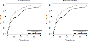
ROC curve (true positive rate versus false positive rate) from a logit model, using forward (on the left) and backward (on the right) stepwise selection.
> pred.train <- prediction(train.db$forward.bic,train.db$class)
> pred.valid <- prediction(valid.db$forward.bic,valid.db$class)
> perf.train <- performance(pred.train,"tpr", "fpr")
> perf.valid <- performance(pred.valid,"tpr", "fpr")
> plot(perf.train,col="grey",lty=2,main="Forward selection")
> plot(perf.valid,add=TRUE)
> legend("bottomright",c("Training dataset","Validation dataset"),
+ lty=c(2,1),col=c("grey","black"),lwd=1)
4.2.4 Leaps and Bounds
The leaps() function (from the eponym library) will search for the best subsets of our predictors using whichever criterion (e.g. Mallows' Cp), according to the leaps and bounds algorithm of Furnival & Wilson (1974). For each p ≥ 1, we are looking for the nbest (here = 1) subset(s) of p predictors, giving the model(s) with the least Mallows' Cp (method = "Cp"). The difference with forward and backward selection is in the search without the constraint that the models are nested. Conversely, the limitation of the leaps() function is that it only applies on numeric variables, so that qualitative variables must be replaced by the indicators of their modalities.
> train.db <- credit.ffindex,]
> y <- as.numeric(train.db[,"class"])
> x <- data.frame(model.matrix(~.,data=train.db[,-which(names(train.db)=="class")]))
> library(leaps)
> selec <- leaps(x,y,method="Cp",nbest=1,strictly.compatible=FALSE)
$label
[1] "(Intercept)" "X.Intercept." "checking_statusA12"
[4] "checking_statusA13" "checking_statusA14" "duration.15.36."
[7] "duration.36.Inf." "credit_historyA31" "credit_historyA32"
[10] "credit_historyA33" "credit_historyA34" "purposeA41"
[13] "purposeA410" "purposeA42" "purposeA43"
[16] "purposeA44" "purposeA45" "purposeA46"
[19] "purposeA48" "purposeA49" "credit_amount.4e.03.Inf.
[22] "savingsA62" "savingsA63" "savingsA64"
[25] "savingsA65" "employmentA72" "employmentA73"
[28] "employmentA74" "employmentA75" "installment_rate"
[31] "personal_statusA92" "personal_statusA93" "personal_statusA94"
[34] "other_partiesA102" "other_partiesA103" "residence_since"
[37] "property_magnitudeA122" "property_magnitudeA123" "property_magnitudeA124"
[40] "age.25.Inf." "other_payment_plansA142" "other_payment_plansA143"
[43] "housingA152" "housingA153" "existing_credits"
[46] "jobA172" "jobA173" "jobA174"
[49] "num_dependents" "telephoneA192"
$size
[1] 2 3 4 5 6 7 8 9 10 11 12 13 14 15 16 17 18 19 20 21 22 23 24 25 26 27
[27] 28 29 30 31 32 33 34 35 36 37 38 39 40 41 42 43 44 45 46 47 48 49
$Cp
[1] 137.62062 123.29162 99.42835 91.94227 83.88375 75.48833 68.37060 62.53615
[9] 56.87359 50.73275 45.06511 40.25486 35.35416 31.38907 27.05092 23.97690
[17] 22.20806 18.48098 16.26368 15.07004 14.41763 13.70477 12.71125 12.30494
[25] 12.50403 12.90835 13.54865 14.52072 15.62970 16.92261 18.08451 19.45329
[33] 20.94871 22.35779 23.81829 25.37059 26.99681 28.71035 30.51637 32.34840
[41] 34.23233 36.14711 38.08677 40.03967 42.01328 44.00346 46.00022 48.00000
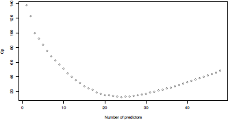
> plot(selec$size-1,selec$Cp, xlab="Number of predictors",ylab="Cp")
The 'best model' is the one that minimized Mallows's Cp (achieved with twenty-four predictors)
> best.model <- selec$which[which((selec$Cp == min(selec$Cp))),]
> z <- cbind(x,y)
> formula <- as.formula(paste("y ~",paste(colnames(x)[best.model],
collapse="+")))
> logit <- glm(formula,data=z,family=binomial(link ="logit"))
> summary(logit)
Call:
glm(formula = formula, family = binomial(link = "logit"), data = z)
Deviance Residuals:
Min 1Q Median 3Q Max
-2.3227 -0.6496 -0.3258 0.6392 2.7946
Coefficients:
Estimate Std. Error z value Pr(>|z|)
(Intercept) 1.5531 0.6064 2.561 0.010425 *
checking_statusA12 -0.5222 0.2731 -1.912 0.055842 .
checking_statusA13 -0.8492 0.4417 -1.922 0.054572 .
checking_statusA14 -2.0301 0.2944 -6.896 5.35e-12 ***
duration.15.36. 1.1469 0.2579 4.447 8.70e-06 ***
duration.36.Inf. 1.2799 0.4501 2.843 0.004463 **
credit_historyA32 -0.5860 0.3772 -1.553 0.120308
credit_historyA33 -0.7710 0.5008 -1.540 0.123667
credit_historyA34 -1.3136 0.4092 -3.210 0.001327 **
purposeA41 -2.1981 0.4774 -4.605 4.13e-06 ***
purposeA410 -16.7122 622.6691 -0.027 0.978588
purposeA42 -1.2116 0.3175 -3.817 0.000135 ***
purposeA43 -1.3125 0.3067 -4.280 1.87e-05 ***
purposeA48 -2.0075 1.2321 -1.629 0.103236
purposeA49 -1.0524 0.3815 -2.758 0.005808 **
credit_amount.4e.03.Inf. 0.9020 0.3153 2.861 0.004227 **
savingsA64 -1.0801 0.5886 -1.835 0.066531 .
savingsA65 -1.1594 0.3185 -3.640 0.000273 ***
employmentA72 0.4903 0.2718 1.804 0.071253 .
installment_rate 0.3088 0.1073 2.878 0.004008 **
other_partiesA103 -1.6873 0.6111 -2.761 0.005760 **
age.25.Inf. -0.7495 0.2793 -2.683 0.007286 **
other_payment_plansA142 -1.1945 0.5500 -2.172 0.029868 *
other_payment_plansA143 -0.9798 0.2973 -3.296 0.000981 ***
housingA152 -0.3106 0.2462 -1.262 0.207072
---
Signif. codes: 0 *** 0.001 ** 0.01 * 0.05 . 0.1 1
(Dispersion parameter for binomial family taken to be 1)
Null deviance: 786.45 on 643 degrees of freedom
Residual deviance: 546.44 on 619 degrees of freedom
AIC: 596.44
Number of Fisher Scoring iterations: 14
We can compute the performance of this model on the validation sample using the AUC criterion:
> xp <- data.frame(model.matrix(~.,data=valid.db[,-which(names(valid.db)=="class")]))
> predclass <- predict(logit,newdata=xp,type="response")
> pred <- prediction(predclass,valid.db$class,label.ordering=c(0,1))
> performance(pred,"auc")@y.values[[1]]
[1] 0.7249934
or by plotting the ROC curve, in Figure 4.7,
> pred.train=prediction(predict(logit,newdata=x,type="response"),train.db$class)
> pred.valid=prediction(predict(logit,newdata=xp,type="response"),valid.db$class)
> perf.train=performance(pred.train,"tpr", "fpr")
> perf.valid=performance(pred.valid,"tpr", "fpr")
> plot(perf.train,col="grey",lty=2,main="Logit model selected with leaps")
> plot(perf.valid,add=TRUE)
> legend("bottomright",c("Training dataset","Validation dataset"),
+ lty=c(2,1),col=c("grey","black"),lwd=1)
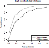
ROC curve obtained using the leaps() procedure, for the model that minimizes Mallows's Cp.
We notice that the model minimizing Mallows' Cp on the training sample is not that one maximizing AUC on the validation sample.
4.2.5 Smoothing Continuous Covariates
So far, we have seen how to model credit applications using categorical variables. But instead of categorizing continuous variables, it could be interesting to keep them as continuous. Categorizing probably makes the model simpler to estimate, and interpret. But there might be serious drawbacks, as discussed in Royston et al. (2006), the main reason being that cutpoints are arbitrary and manipulable (and can result in both positive and negative associations, as mentioned in Wainer (2006)), unless we specify the cutpoints based on the proportion of data in each category of the predictor. As claimed in Harrell (2006), “a better approach that maximizes power and that only assumes a smooth relationship is to use a restricted cubic spline function for predictors that are not known to predict linearly.” Nevertheless, one has to admit that having, at the same time, a large number of categorical and continuous variables might yield complex and unstable models. So, smoothing continuous covariates will mainly be discussed to introduce some statistical techniques.
Consider a logistic regression on two continuous variates: the duration D and the age A. Then with a logistic regression,
This is a linear model because a linear combination of explanatory variates is considered
> regglm <- glm(class~age+duration,data=credit[index,],family=binomial(link="logit"))
> summary(regglm)
Call:
glm(formula = class ~ age + duration, family = binomial(link = "logit"),
data = credit[index,])
Deviance Residuals:
Min 1Q Median 3Q Max
-1.5814 -0.8382 -0.7007 1.2380 2.0974
Coefficients:
Estimate Std. Error z value Pr(>|z|)
(Intercept) -1.106634 0.342223 -3.234 0.00122 **
age -0.017866 0.008673 -2.060 0.03941 *
duration 0.039913 0.007172 5.565 2.62e-08 ***
---
Signif. codes: 0 *** 0.001 ** 0.01 * 0.05 . 0.1 1
(Dispersion parameter for binomial family taken to be 1)
Null deviance: 786.45 on 643 degrees of freedom
Residual deviance: 750.43 on 641 degrees of freedom
AIC: 756.43
Number of Fisher Scoring iterations: 4
In those Generalized Linear Models, we considered the following (linear) relationship, based on link function g:
The idea now is to use non-parametric techniques to estimate h : where
Generalized Additive Models consider restricted a class of functions, namely those that have an additive form:
As described in Wood (2006), the gam function of package mgcv can be used to estimate function h, using the Lanczos algorithm. The generic code is
> library(mgcv)
> reggam <- gam(Y~s(X1),data=db,family=binomial(link="logit"))
> reggam <- gam(Y~s(X1,by=F1),data=db,family=binomial(link="logit"))
> reggam <- gam(Y~s(X1)+s(X2),data=db,family=binomial(link="logit"))
> reggam <- gam(Y~s(X1,X2),data=db,family=binomial(link="logit"))
where X1 and X2 are continuous covariates, while F1 denotes some factor. Some arguments can be added to the s() function, but the default option is to use a cubic spline basis and to automatically choose the smoothing parameter via generalized cross validation. The idea of a cubic spline regression (see Wood (2006) for more details), with k knots {ξ1, ...,ξk} is to start with a cubic polynomial regression, on X1, X21 and X13, and then to add a truncated power basis function for each knot, is equal to x if , and 0 otherwise. A cubic spline regression is a standard regression on k + 3 regressors (and the intercept).
Here, consider a bivariate spline smoothing function on the two (continuous) covariates,
> reggam <- gam(class~s(age,duration),data=credit[index,],family=binomial(link="logit"))
In order to compare the two models, regglm and reggam, it is possible to plot the predicted value of ?(Y|A, D):
> pglm <- function(x1,x2){return(predict(regglm,newdata=
+ data.frame(duration=x1,age=x2),type="response"))}
> pgam <- function(x1,x2){return(predict(reggam,newdata=
+ data.frame(duration=x1,age=x2),type="response"))}
> M <- 31
> cx1 <- seq(from=min(credit$duration), to=max(credit$duration), length=M)
> cx2 <- seq(from=min(credit$age), to=max(credit$age), length=M)
> Pgam <- outer(cx1,cx2,pgam)
> persp(cx1,cx2,Pgam)
> contour(cx1,cx2,Pgam)
The output for these two models can be visualized in Figure 4.8.

Linear (on top, with glm) versus nonlinear (below, with gam) logistic regression, on the duration and the age.
4.2.6 Nearest-Neighbor Method
Another popular tool to classify with a non-parametric model is to use the k-th nearest- neighbor method. The use of this classifier in credit scoring was discussed, for instance, in Henley & Hand (1996).
Given our two covariates X = (A, D), the idea is to obtain a prediction for some x to consider the average of Y over the k-nearest neighbors Xi close to x, for some distance d (such as the Euclidean distance). More precisely, if
denote the k closest points Xi to x in the training sample, then
> pkmeans <- function(x1,x2,k=25){
Linear (on top, with glm) versus nonlinear (below, with gam) logistic regression, on the duration and the age.
> D <- as.matrix(dist(rbind(credit[index,c("duration","age")],
+ c(x1,x2))))[length(index)+1,1:length(index)]
> i <- as.vector(which(D<=sort(D)[k]))
> return(mean((credit[index,"class"])[i]))}
4.3 Penalized Logistic Regression: From Ridge to Lasso
In the previous section, we have seen that β's in the logistic regression were obtained by maximizing the log-likelihood. But is it possible to add some penalty function, as discussed in Fu (1998) for instance,
for some parameter and where p is the so-called penalty function. Penalizing the log-likelihood is common when the number of explanatory variable is large, or when those variables are correlated. The general form is, for
where we obtain a ridge model when α = 0 (L2 norm) and a lasso model when α = 1 (L1 norm); see Fu (1998). This penalized logistic regression function can found in package glmnet (and also penalized , lasso2 or logistf, even if those packages will not be used in this section).
4.3.1 Ridge Model
The generic code to run a ridge regression, introduced in Hoerl & Kennard (1970), is obtained when α is null, obtained setting alpha=0,
> library(glmnet)
> ridge <- glmnet(x,y,alpha=0,family ="binomial",lambda=c(0,1,2),standardize = TRUE)
Parameter λ can be estimated using cross-validation techniques, after having created indicators as glmnet function applies to numeric variables.
> train.db <- credit.rcd[index,]
> yt <- as.numeric(train.db[,"class"])
> xt <- model.matrix(~ .,data=train.db[,-which(names(train.db)=="class")])
>set.seed(235)
> cvfit <- cv.glmnet(xt,yt,alpha=0, family = "binomial",type="auc",nlambda=100)
>cvfit$lambda.min
[1]0.03983943
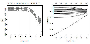
cvfit$lambda.min is the value of lambda giving the minimal error, viz here the maximal area below the ROC curve. On Figure 4.10 is represented the area below the ROC curve, for varying λ. The code is

Nearest-neighbor method used to predict the probability that class will be equal to 1, on the duration and the age.

> plot(cvfit)
> abline(v=log(cvfit$lambda.min),col='blue',lty=2)
It is also possible to visualize the evolution of parameters estimates as a function of λ.
> fits <- glmnet(xt,yt,alpha=0,family = "binomial",lambda=seq(cvfit$lambda[1],
+ cvfit$lambda[100],length=10000),standardize = TRUE)
> plot(fits,xvar="lambda",label="T")
So far, we have use only the training sample. But it is also possible to see on the validation sample how those models actually perform:
> valid.db <- credit.rcd[-index,]
> yv <- as.numeric(valid.db[,"class"])
> xv <- model.matrix(~ .,data=valid.db[,-which(names(train.db)=="class")])
> yvpred <- predict(fits,newx=xv,type="response")
> library(ROCR)
> roc <- function(x) {performance(prediction(yvpred[,x],yv),"auc")@y.values[[1]]}
> vauc <- Vectorize(roc)(1:ncol(yvpred))
> fits$lambda[which.max(vauc)]
[1] 2.137035
It is possible to visualize the AUC as a function of λ (Figure 4.11):

> plot(fit$lambda,vauc,type="l")
and we can get the maximal AUC obtained on the validation sample:
> vauc[which.max(vauc)]
4.3.2 Lasso Regression
The lasso regression, introduced in Tibshirani (1996), is obtained when α is one:
> lasso <- glmnet(x,y,alpha=1,family ="binomial",lambda=c(0,1,2),standardize = TRUE)
Again, parameter can be estimated using cross-validation techniques:
> set.seed(235)
> cvfit <- cv.glmnet(xt,yt,alpha=1, family = "binomial",type="auc",nlambda=100)
> cvfit$lambda.min
[1] 0.00217614
which can be visualized on Figure 4.12, representing the area below the ROC curve, for varying λ, using
> plot(cvfit)
> abline(v=log(cvfit$lambda.min),col=''grey'',lty=2)
It is also possible to visualize the evolution of parameters estimates as a function of λ:
> fits <- glmnet(xt,yt,alpha=0,family = "binomial",lambda=seq(cvfit$lambda[1],
+ cvfit$lambda[71],length=10000),standardize = TRUE)
> plot(fits,xvar="lambda",label="T")
Ridge regression has a major disadvantage: Unlike stepwise selection (which will generally suggest to consider only a subset of the covariables), ridge regression will include all predictors in the final model. Prediction will be good, but it might be a challenge to interpret values, and signs, when the number of regressors is large. Even if a model with three variables is relevant, with ridge regression, all variables will be considered. Increasing the value of λ will tend to reduce the magnitudes and the importance of the coefficients, but will not result in the exclusion of any of the variables. On the other hand, lasso performs variable selection, so models generated from the lasso are generally much easier to interpret than those produced by ridge regression. As claimed in Hastie et al. (2009), lasso yields sparse models.
4.4 Classification and Regression Trees
In the first part, we have used a logistic regression to compute the probability P(Y|X), given some covariates. Another class of popular predictive models is the class of regression trees and classification trees, introduced by Breiman et al. (1984). The latter technique will be described in this section (regression trees are used when the variable of interest is continuous, while classification trees are used for binary response); and in the next section, we will mention some so-called ensemble methods, that construct more than one decision tree:
- Bagged trees, which build multiple classification or regression trees, by repeatedly resampling training data with replacement;
- The random forest classifier, which uses multiple classification or regression trees, in order to minimize the error, by repeatedly resampling both training data (as in bagging) and predictors in building the trees,
- Boosted trees, which build multiple classification or regression trees on repeatedly modified versions of the data, before combining these trees through a weighted majority vote or weighted mean to produce the final prediction; the data modifications consist of applying weights to each of the training observations, with increased weights for misclassified observations and decreased weights otherwise.
4.4.1 Partitioning
In order to illustrate the use of trees, consider as in Sections 4.2.5 and 4.2.6, two continuous variates: the duration and the age, denoted (with very general notations) X1 and X2 respectively.
> X1 <- credit[,"age"]
> X2 <- credit[,"duration"]
> Y <- credit[,"class"]
Starting with all the data, consider a splitting variable j (here in {1, 2}), and a split point s (within the range of variable ). Define then the pair of half-planes
and
where Xj,i is the i-th value of variable Xj. If we adopt as a criterion minimization of the sum of squares (the choice of the criterion will be discussed in the next section), we seek the splitting variable j and split point s that solve
Note that computation here is easy because for any choice j and s, the inner minimization is solved with
and
where n±(j, s) denotes the cardinal of partition P±(j, s). Thus, for each variable, the splitting point is obtained by scanning through possible outputs.
> criteria1 <- function(s){
+ sum((Y[X1<=s]-mean(Y[X1<=s]))"2)+sum((Y[X1>s]-mean(Y[X1>s]))"2)}
> criteria2<- function(s){
+ sum((Y[X2<=s]-mean(Y[X2<=s]))"2)+sum((Y[X2>s]-mean(Y[X2>s]))"2)}
It is possible to visualize those sums using
> S <- seq(0,100,length=501)
> plot(S,Vectorize(criteria2)(S),type="l",ylab="Sum of squares",xlab="Splitting point")
> lines(S,Vectorize(criteria1)(S),type="l",lty=2)
> legend(70,205,c("Variable X1","Variable X2"),lty=2:1)
Here, the best partition is obtained when the split is done according to the second variate (the duration of the credit), and where s is in [33, 36) (here, the minimum is not unique as age and duration are discrete variables).
> S[which(Vectorize(criteria2)(S)==min(Vectorize(criteria2)(S)))]
[1] 33.0 33.2 33.4 33.6 33.8 34.0 34.2 34.4
[9] 34.6 34.8 35.0 35.2 35.4 35.6 35.8
Thus, it might be optimal to consider the midpoint of this interval, s* = 34.5, on variable X2.
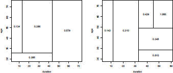
Having found the best split (at least for this specific criterion, that yields the partition on the left of Figure 4.14), we partition the data into the two resulting regions, and repeat this splitting process on each of the two regions. And then, the process is repeated (again and again) on all of the resulting regions. For the second split, four cases should be considered, that can be visualized on the right of Figure 4.14
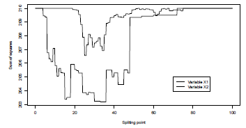
Evolution of the sum of squares, when the population is split into two groups, either age<=s and age>s, or duration<=s and duration>s.
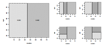
Regions obtained at the first splitting point, on the left, and possible regions obtained after the second splitting, on the right.
The following code can be used:
> s.star <- 34.5
> criteria1.lower <- function(s){
+ sum((Y[(X1<=s)&(X2<=s.star)]-meanY[((X1<=s)&(X2<=s.star)]))"2)+
+ sum((Y[(X1>s)&(X2<=s.star)]-meanY[((X1>s)&(X2<=s.star)]))"2) +
+ sum((Y[(X2>s.star)]-mean Y[((X2>s.star)]))"2)}
> criteria1.upper <- function(s){
+ sum((Y[(X1<=s)&(X2>s.star)]-mean((Y[X1<=s)&(X2>s.star)]))"2)+
+ sum((Y[(X1>s)&(X2>s.star)]-mean((Y[X1>s)&(X2>s.star)]))"2) +
+ sum((Y[(X2<=s.star)]-mean(Y[(X2<=s.star)]))"2)}
> criteria2 <- function(s){
+ sum((Y[(X2<=s)&(X2<=s.star)]-mean(Y[(X2<=s)&(X2<=s.star)]))"2)+
+ sum((Y[(X2>s)&(X2<=s.star)] -mean(Y[(X2>s)&(X2<=s.star)]))"2)+
+ sum((Y[(X2<=s)&(X2>s.star)]-mean(Y[(X2<=s)&(X2>s.star)]))"2)+
+ sum((Y[(X2>s)&(X2>s.star)] -mean(Y[(X2>s)&(X2>s.star)]))"2)}
Here, the minimum of those three functions is again obtained when splitting is done according to the duration, and the splitting value is
> S[which(Vectorize(criteria2)(S)==min(Vectorize(criteria2)(S)))]
[1] 11.0 11.2 11.4 11.6 11.8
Thus, it might be optimal to cut at the midpoint, s* = 11.5. Etc.
This splitting procedure can be done using function tree of library tree,
> library(tree)
> Tree <- tree(class~age+duration,data=credit)
> Tree
node), split, n, deviance, yval * denotes terminal node
1) root 1000 210.00 0.3000
2) duration <34.5 830 160.70 0.2627
4) duration < 11.5 180 22.95 0.1500 *
5) duration > 11.5 650 134.90 0.2938 *
3) duration > 34.5 170 42.45 0.4824
6) age < 29.5 58 12.78 0.6724 *
7) age > 29.5 112 26.49 0.3839 *
The first node is here based on the duration, and the splitting value is 34.5. For the second one, we can either
- Consider the half-space with low durations, and then the optimal partition is based (again) on duration, with a splitting value equal to 11.5, or
- Consider the half-space with large durations, and then the optimal partition is based on age, with a splitting value equal to 29.5
This tree can be visualized on Figure 4.15 using
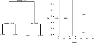
> plot(Tree)
> text(Tree)
while the partition (and the empirical probability that Y is 1) can be visualized using
> partition.tree(Tree)
Consider a loan of 20 months. On the right of Figure 4.15, we can see that the probability that class is equal to 1 is here 29.4%. On the tree (graph on the left of Figure 4.15) it is obtained going first on the left, as yes duration<34.5, and then on the right as no duration<11.5. The probability is then the second value at the bottom, 29.38%.
Those four regions (denoted 4, 5, 6 and 7 in the output) are called terminal nodes, or, if we keep a tree analogy, leaves of the tree. And decision trees are usually drawn upside down, with leaves at the bottom of the tree.
4.4.2 Criteria and Impurity
Assume that we have reached a node P, and we wonder if we should split it, or not. In a perfect world, all the population in the leaf will be identical, that is, either people where Y = 0 or Y = 1. In that case, p = ℙ(Y = 1 |P) will be either 0 or 1. The node will be be said to be pure. Conversely, the worst case scenario would be when half of the population is 0 and half is 1. In that case, p =1/2 and the node would be said to be highly impure. Formally, impurity of a node is a function of ℙ(Y = 1|P). Natural assumptions on are that is positive, symmetric, and minimal when the probability is either 0 or 1. Standard functions are
- Bayes error
- cross-entropy function
- Gini index
These three functions are concave; they have minimums at 0 and 1, and maximum at 1/2.
As explained in Breiman et al. (1984), the Gini index is extremely popular to partition the data.
To illustrate the use of these functions, consider the very first partition. As mentioned earlier, if we split according to variable j, at splitting point s, two samples are obtained, in two half-spaces:
and
In each region, define where
and
The entropy impurity is then the sum of
while the Gini index is the sum of
.
These indices can be computed on contingency tables, as described in Table 4.2.
Contingency table and tree partitioning (first step), based on variable Xj.
Value of Y |
||
Y=1 |
Y=0 |
|
The code to produce this table (on the second variable, and with splitting value s = 35) is simply
> s <- 35
> X0 <- (X2<=s)
> (T <- table(X0,Y))
Y
X0 0 1
FALSE 88 82
TRUE 612 218
The Gini index is then computed using the following code:
> Nx <- apply(T,1,sum)
> (Pxy <- T/matrix(rep(Nx,2),2,nrow(T)))
Y
X0 0 1
FALSE 0.5176471 0.4823529
TRUE 0.7373494 0.2626506
> Vxy <- Pxy*(1-Pxy)
> sum(Nx/sum(T)*apply(Vxy,1,sum))
[1] 0.4063785
This criterion can be used also to see how to split the population:
> gini <- function(X0){
+ T <- table(X0,Y)
+ Nx <- apply(T,1,sum)
+ Pxy <- T/matrix(rep(Nx,2),2,nrow(T))
+ Vxy <- Pxy*(1-Pxy)
+ return(sum(Nx/sum(T)*apply(Vxy,1,sum)))}
> criteria1=function(s){gini(X1<s)}
> criteria2=function(s){gini(X2<s)}
and as previously, it is possible to plot these indices for all s:
> S <- seq(0,80,length=501)
> plot(S,Vectorize(criteria2)(S),type="l,ylab=Gini index",xlab="Spliting point")
> lines(S,Vectorize(criteria1)(S),type="l",lty=2)
> legend(55,.408,c("Variable X1","Variable X2"),lty=2:1)
Again, we can see that the minimum is obtained when splitting variable X2 is at some splitting point s ∈ [33, 36), as on Figure 4.13
Based on a set of predictors, for instance
> predictors <- names(credit)[-20]
run
> cart <- rpart(class ~ . ,data = credit[index,c("class",predictors)],
+ method="class",parms=list(split="gini"),cp=0)
> printcp(cart)
Classification tree:
rpart(formula = class ~ ., data = credit[index, c("class", predictors)],
method = "class", parms = list(split = "gini"), cp = 0)
Variables actually used in tree construction:
[1] age checking_status credit_amount
[4] credit_history duration employment
[7] job other_payment_plans property_magnitude
[10] purpose residence_since savings
Root node error: 193/644 = 0.29969
n= 644
CP nsplit rel error xerror xstd
1 0.0595855 0 1.00000 1.00000 0.060237
2 0.0518135 2 0.88083 1.00000 0.060237
3 0.0328152 3 0.82902 0.97409 0.059781
4 0.0310881 6 0.73057 0.96373 0.059592
5 0.0155440 8 0.66839 0.95337 0.059400
6 0.0138169 11 0.62176 0.99482 0.060148
7 0.0129534 14 0.58031 0.99482 0.060148
8 0.0103627 17 0.53886 0.99482 0.060148
9 0.0069085 18 0.52850 1.02591 0.060674
10 0.0051813 21 0.50777 1.02591 0.060674
11 0.0025907 26 0.48187 1.04663 0.061008
12 0.0000000 28 0.47668 1.05181 0.061090
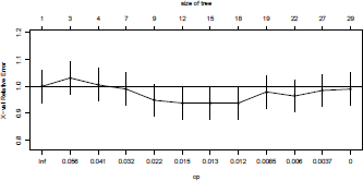
It is possible to visualize the Complexity Parameter Table (Figure 4.16) using
> plotcp(cart)
Finally, in order to assess the quality of the model, it is possible to plot the ROC for the tree obtained using library rpart (on the left) and library party (on the right) on Figure 4.18:
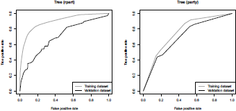
ROC curve (true positive rate versus false positive rate) from two classification trees, obtained using packages rpart and party.
> train.db$pred.tree <- predict(cart,type='prob',newdata=train.db)[,"1"]
> valid.db$pred.tree <- predict(cart,type='prob',newdata=valid.db)[,"1"]
> library(ROCR)
> pred.train=prediction(train.db$pred.tree,train.db$class)
> pred.valid=prediction(valid.db$pred.tree,valid.db$class)
> perf.train=performance(pred.train,"tpr", "fpr")
> perf.valid=performance(pred.valid,"tpr", "fpr")
> plot(perf.train,col="grey",lty=2,main="Tree (rpart)")
> plot(perf.valid,add=TRUE)
> library(party)
> ct.arbre <- ctree_control(mincriterion =0.95,
+ minbucket=10,minsplit=10*2,maxdepth=0)
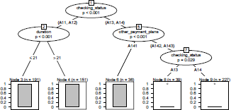
> ctree <- ctree(class ~ .,data = credit[index,c("class",predictors)],control=ct.arbre)
> plot(ctree)
> train.db$pred.tree <- unlist(predict(ctree,type='prob',newdata=train.db))
> valid.db$pred.tree <- unlist(predict(ctree,type='prob',newdata=valid.db))
> pred.train=prediction(train.db$pred.tree,train.db$class)
> pred.valid=prediction(valid.db$pred.tree,valid.db$class)
> perf.train=performance(pred.train,"tpr", "fpr")
> perf.valid=performance(pred.valid,"tpr", "fpr")
> plot(perf.train,col="grey",lty=2,main="Tree (party)")
> plot(perf.valid,add=TRUE)
Finally, note that it is also possible to use prune trees, to avoid overfitting the data, using a tree size that minimizes the cross-validated error (the xerror column printed by printcp), here
> prunecart <- prune(cart,cp=.015)
Nice graphs can be produced using functions of the rpart.plot package, such as prp()
> plot(prunecart,branch=.2, uniform=TRUE, compress=TRUE,margin=.1)
> text(prunecart, use.n=TRUE,pretty=0,all=TRUE,cex=.5)
> library(rpart.plot)
> prp(prunecart,type=2,extra=1)
Several other functions can be used on rpart objects; see Galimberti et al. (2012), Archer (2010).
4.5 From Classification Trees to Random Forests
Trees are nice, as they are extremely easy to understand. Unfortunately, trees are extremely volatile: If we split the training data into two parts (randomly) and fit decision trees to both halves, the output could be quite different (see Figure 4.20).

> library(tree)
> set.seed(l)
> indextree <- sample(1:1000,size=500,replace=FALSE)
> t1 <- tree(class~age+duration,data=credit[indextree,])
> t2 <- tree(class~age+duration,data=credit[-indextree,])
> partition.tree(t1)
> partition.tree(t2)
A natural idea is then to use bootstrap aggregation (called bagging) to reduce variance.
4.5.1 Bagging
The idea of bagging (from bootstrap aggregating) was proposed in Breiman (1996). This bagging procedure involves the following steps:
- Create multiple copies of the original training dataset using bootstrap procedures.
- Fit classification trees to each copy.
- Aggregate (or combine) all of the trees in order to create a single predictive model.
> library(ipred)
> set.seed(123)
> bag1 <- bagging(class ~ .,data=credit[index,c("class",predictors)],nbagg=200,coob=TRUE,
+ control= rpart.control(minbucket=5))
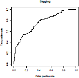
> pred=prediction(predict(bagi, test, type="prob",
+ aggregation="average"),credit[-index,"class"])
> perf=performance(pred,"tpr", "fpr")
4.5.2 Boosting
When bagging trees, boostrap techniques were considered, meaning that all copies were independent, so trees were built independently of the others. Boosting will work in a similar way, except that trees are grown sequentially: Each tree is grown using information obtained from previously grown trees. Thus, boosting does not involve bootstrap sampling, and each tree is obtained from a modified version of the original dataset.
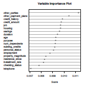
Variable importance can be visualized using functions ada from the eponym library for boosting, and then varplot (see e.g. Culp et al. (2006) for more details). Boosting will be interesting only in the case where several predictors are important.
> library(ada)
> set.seed(123)
> boost <- ada(class ~ data=credit[index,c("class",predictors)],
+ type="discrete", loss="exponential", control =
+ rpart.control(cp=0), iter = 5000, nu = 1,
+ test.y=test[,"class"], test.x=test[,1:19])
> varplot(boost,type="scores")
other_parties other_payment_plans credit_history credit_amount job
0.011265924 0.010419375 0.009860286 0.009756094 0.009687740
housing savings duration age
0.009686706 0.009603497 0.009422427 0.009276642
purpose num_dependents existing_credits personal_status employment
0.009250920 0.009223420 0.009177000 0.009072014 0.008770979
property_magnitude residence_since installment_rate checking_status telephone
0.008407637 0.008280839 0.008194080 0.007814246 0.007088610
4.5.3 Random Forests
The drawback of the bagging technique is that variance reduction is usually small. The intuitive idea behind this is simple: Assume that we have in our model one very strong predictor, and a couple of moderately strong ones. Using bagging technique will grow trees quite similar. Therefore, predictions will be extremely correlated. And averaging extremely correlated variables does not lead to a significant reduction in the variance.
The last method we will discuss provides an improvement over bagged trees that decorrelates the trees. In building a random forest, at each split in the tree, the algorithm is not allowed to consider all the available predictors.
In order to avoid this problem, random forest algorithms force us to consider only a subset of predictors. Then predictions will have more variability, and aggregation will then be extremely efficient. Resulting trees are then usually less variable, and hence more reliable.
The package randomForest (see Liaw & Wiener (2002)) can be used to build a predictive model.
> library(randomForest)
> set.seed(123)
> rf <- randomForest(class ~ ., data=credit[index,c("class",predictors)],
+ importance=TRUE, ntree=500, mtry=3, replace=TRUE, keep.forest=TRUE,
+ nodesize=5, ytest=test[,"class"], xtest=test[,1:19])
Message d'avis :
In randomForest.default(m, y, ...) :
The response has five or fewer unique values.
Are you sure you want to do regression?
> rf
Type of random forest: regression
Number of trees: 500
No. of variables tried at each split: 3
Mean of squared residuals: 0.1638417
% Var explained: 21.93
Test set MSE: 0.17 %
% Var explained: 19.74
Then, the extractor function for variable importance measures as produced by the previous function can be obtained using either type=1 for mean decrease in accuracy,
> importance(rf,type=1)
%IncMSE
checking_status 26.8158301
duration 17.2268269
credit_history 6.8096722
purpose 8.4606150
credit_amount 6.4029995
savings 6.7660725
employment 2.9760754
installment_rate 4.6122336
personal_status 2.2104102
other_parties 4.2947555
residence_since 1.5007471
property_magnitude 0.8281632
age 5.5388709
other_payment_plans 8.0462958
housing 4.1083429
existing_credits 2.1720201
job -0.4039036
num_dependents -0.1864291
telephone 1.0709050
or type=2 for mean decrease in node impurity,
> importance(rf,type=2)
NodePurity
checking_status 14.712959
duration 11.359640
credit_history 6.876229
purpose 11.722564
credit_amount 12.257516
savings 6.135412
employment 6.780975
installment_rate 4.467483
personal_status 4.371698
other_parties 1.960203
residence_since 3.710073
property_magnitude 5.003570
age 10.680848
other_payment_plans 3.843822
housing 3.374496
existing_credits 2.307880
job 3.392985
num_dependents 1.067552
telephone 1.798760