
Chapter 2
Standard Statistical Inference
Christophe Dutang
Université de Strasbourg and Université du Maine, Le Mans, France
Strasbourg, France
2.1 Probability Distributions in Actuarial Science
Let X be our quantity of interest. Actuarial models rely on particular assumptions on the probability distribution of X. When X represents the claim amount or the life length of an individual, one expects X to have a distribution ℝ+, whereas when X represents the claim number, we deal with distribution on ℕ. But, characterizing the support of the random variable X is a necessary but not a sufficient step to characterize our quantity of interest.
In the discrete case, probability distributions are generally characterized by the mass probability function px or the “elementary” probabilities: px(x)=ℙ(X=x) for x∈ℕ In the continuous case, we define the probability distribution by its density fx(x), being the infinitesimal version px such that fx(x)dx=ℙ(X∈[x,x+dx]). A third case is when the random variable has both continuous and discrete parts, for which there is no proper density. In such a case, we define the distribution with the cumulative distribution function FX(x)=ℙ(X≤x). We recall that for a discrete distribution on ℕ FX(x)=Σ[x]n=0pX(n) while for a continuous distribution, FX(x)=∫X−∞fx(y)dy.
The purpose of this section is to present the most common distributions used in actuarial sciences, being continuous, discrete or mixed-type. As always in this book, a special emphasis is put on how this topic is implemented and can be extended in R.
2.1.1 Continuous Distributions
There are a lot of ways to classify and to distinguish distributions. We present here the Pearson system and the exponential family, the latter being used, for instance, in generalized linear models (GLM, see Chapter 14). Pearson (1895) considers the family of continuous distributions such that the density function fX verifies the following ordinary differential equation:
1fx(x)dfx(x)dx=−a+xc0+c1x+c2x2
where a,c0,c1,c2 are constants. Let p(x) = c0 + c1x + c2 x2. The solution is defined up to a constant K which is derived by the constraint ∫ℝfX(x)dx=1. Type 0 is obtained when c1 = c2 = 0: we get fX(x)=Ke−(2a+∞)∞/(2c0) fX(x)=Ke−(2a+∞)∞/(2c0). , which is the the normal distribution. Type 1 is the case where the polynomial function c0 + c1x + c2 x2 has two distinct real roots a1 and a2 such that a1 < 0 < a2: we get fX(x)=K(x−a1)m1(a2−x)m2. We recognize the beta distribution. Type 2 corresponds to the case where m1 = m2 = m.
Type 3 is obtained when c2 =0 leading a first-order polynomial function c0 + c1x. In this case, we get the gamma distribution with fX(x)=K(c0+c1x)me∞+c1 fX(x)=K(c0+c1x)mex+c1. . Type 4 corresponds to the case where the polynomial function p(x) = c0 + c1x + c2x2 has no real roots, in which case p(x) = C0 + c2(x + C1)2. We get fX(x)=K(c0+c2(x+c1)2)ektan−1((x+c1)/√c0/c2), which is closely linked to the generalized inverse Gaussian distribution of Barndoff-Nielsen.
We get type 5 when p is a perfect square, that is, p(x) = (x + C1)2. The associated density is fX(x)=K(x+C1)−1/c2ek/(x+C1). Two special cases are obtained when k = 0, c2 > 0 for type 8 and c2 < 0 for type 9.
Type 6 is obtained when p has two real roots a1, a2 of the same sign for which we get fX(x)=K(x−a1)m1(x−a2)m2, a generalized Beta distribution. Finally, type 7 is obtained when a = c1 =0, leading to fX(x)K(c0+c2x2)−1/(2c2).
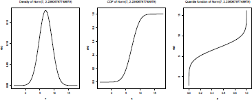
Those distributions are implemented in the package PearsonDS. In Figure 2.1, we plot the densities for the first seven types in order to compare the different possible shapes.

> library(PearsonDS)
> x <- seq(-1, 6, by=1e-3)
> y0 <- dpearson0(x, 2, 1/2)
> y1 <- dpearsonI(x, 1.5, 2, 0, 2)
> y2 <- dpearsonII(x, 2, 0, 1)
> y3 <- dpearsonIII(x, 3, 0, 1/2)
> y4 <- dpearsonIV(x, 2.5, 1/3, 1, 2/3)
> y5 <- dpearsonV(x, 2.5, -1, 1)
> y6 <- dpearsonVI(x, 1/2, 2/3, 2, 1)
> y7 <- dpearsonVII(x, 3, 4, 1/2)
> plot(x, y0, type="l", ylim=range(y0, y1, y2, y3, y4, y5, y7),
+ ylab="f(x)", main="The Pearson distribution system")
> lines(x[y1 != 0], y1[y1 != 0], lty=2)
> lines(x[y2 != 0], y2[y2 != 0], lty=3)
> lines(x[y3 != 0], y3[y3 != 0], lty=4)
> lines(x, y4, col="grey")
> lines(x, y5, col="grey", lty=2)
> lines(x[y6 != 0], y6[y6 != 0], col="grey", lty=3)
> lines(x[y7 != 0], y7[y7 != 0], col="grey", lty=4)
> legend("topright", leg=paste("Pearson", 0:7), lty=1:4,
+ col=c(rep("black", 4), rep("grey", 4)))
Another important class of distribution is the exponential family, that Andersen (1970) traces back to the work of Pitman, Darmois and Koopman in the mid-1930s. This family contains distributions where the density function can be written as
fX(x)=exp(d∑j=1aj(x)αj(θ)+b(x)+β(θ))
where θ∈ℝd is the d-dimensional parameter vector, and aj,αj,bandβ are known functions (see Bickel & Doksum (2001) for more details). The exponential family includes many familiar distributions. We recover the exponential distribution fx(x)=λe−λx with d=1,a(x)=x,α(x)=λ,b(x)=0 and β(λ)=log(λ),or the normal distribution, fX(x)=e−(x−μ)2/(2σ2)/√2πσ2 with d=2,a1(x)=x2,α1(m,σ2)=−1/(2σ2),a2(x)=x, α2(m,σ2)=m/σ2,b(x) and β(m,σ2)=−m/(2σ2)−log√2πσ2. In the exponential family, the gamma and the inverse Gaussian distributions are also examples of particular interest in actuarial science.
In R, each probability distribution is implemented by a set of four functions and a particular root name foo: dfoo computes the density function fx (x) or the mass probability functionpx(x), pfoo the cumulative distribution function Fx(x), qfoo the quantile function F-1xand rfoo a random number generator. For instance, the gamma distribution with density is implemented in dgamma, pgamma, qgamma and rgamma; see example below.
> dgamma(1:2, shape=2, rate=3/2)
[1] 0.5020429 0.2240418
> pgamma(1:2, shape=2, rate=3/2)
[1] 0.4421746 0.8008517
> qgamma(1/2, shape=2, rate=3/2)
[1] 1.118898
> set.seed(1)
> rgamma(5, shape=2, rate=3/2)
[1] 0.553910 2.380504 2.308780 1.367208 2.590273
In Table 2.1, the continuous distributions implemented in Rare listed. This set of distributions is rather limited, and in practice, other distributions such as Pareto are particularly relevant in actuarial science. Most of distributions are generally implemented in a dedicated package. The full list of non R-base distributions are listed on the corresponding task view http://cran.r-project.org/web/views/Distributions.html. Among the numerous packages, two packages focus on distributions relevant to actuarial science : actuar and ActuDistns. Note that actuar provides the raw moment , the limited expected values and the moment generating functions for many distributions in three dedicated functions mfoo, levfoo and mgffoo.
Continuous distributions in R.
Probability Distribution |
Root |
Probability Distribution |
Root |
|---|---|---|---|
Beta |
beta |
Logistic |
logis |
Cauchy |
cauchy |
Lognormal |
lnorm |
Chi-2 |
chisq |
Normal |
norm |
Exponential |
exp |
Student t |
t |
Fisher F |
f |
Uniform |
unif |
Gamma |
gamma |
Weibull |
weibull |
When on a particular problem all classical distributions have been exhausted, it is sometimes appropriate to create new probability distributions. Typical transformations of a random variable X are listed:
- (i) Translation X + c (e.g. the shifted lognormal distribution),
- (ii) Scaling X,
- (iii) Power Xα (e.g. the generalized beta type 1 distribution),
- (iv) Inverse 1/X (e.g. the inverse gamma distribution),
- (v)The logarithm log(X) (e.g. the loglogistic distribution),
- (vi)Exponential exp(X) and
- (vii)The odds ratio X/(1 — X) (e.g. the beta type 2 distribution).
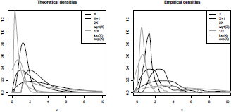
With the small code below, we can visualize all those transformations (except the last one) on gamma-distributed variables, using
g being a monotonic transformation.
> f <- function(x) dgamma(x,2)
> f1 <- function(x) f(x-1)
> f2 <- function(x) f(x/2)/2
> f3 <- function(x) 2*x*f(x"2)
> f4 <- function(x) f(1/x)/x"2
> f5 <- function(x) f(exp(x))*exp(x)
> f6 <- function(x) f(log(x))/x
> x=seq(0,10,by=.025)
> plot(x,f(x), ylim=c(0, 1.3), xlim=c(0, 10), main="Theoretial densities",
+ lwd=2, type="l", xlab="x", ylab="")
> lines(x,f1(x), lty=2, lwd=2)
> lines(x,f2(x), lty=3, lwd=2)
> lines(x,f3(x), lty=4, lwd=2)
> lines(x,f4(x), lty=1, col="grey", lwd=2)
> lines(x,f5(x), lty=2, col="grey", lwd=2)
> lines(x,f6(x), lty=3, col="grey", lwd=2)
> legend("topright", lty=1:4, col=c(rep("black", 4), rep("grey", 3)),
+ leg=c("X","X+1","2X", "sqrt(X)", "1/X", "log(X)", "exp(X)"))
We can also run simulations and visualize kernel-based densities:
> set.seed(123)
> x <- rgamma(100, 2)
> x1 <- x+1
> x2 <- 2*x
> x3 <- sqrt(x)
> x4 <- 1/x
> x5 <- log(x)
> x6 <- exp(x)
> plot(density(x), ylim=c(0, 1), xlim=c(0, 10), main="Empirical densities", + lwd=2, xlab="x", ylab="f_X(x)")
> lines(density(x1), lty=2, lwd=2)
> lines(density(x2), lty=3, lwd=2)
> lines(density(x3), lty=4, lwd=2)
> lines(density(x4), lty=1, col="grey", lwd=2)
> lines(density(x5), lty=2, col="grey", lwd=2)
> lines(density(x6), lty=3, col="grey", lwd=2)
In Figure 2.2, we plot the empirical densities (as estimated by the density() function, using a kernel approach). Note that the exponential transformation has a heavy-tailed distribution and only the right-tail is shown on the graphic. With these transformations in mind, we can now list the set of distributions generally used in actuarial science.
The most important distribution with finite-support is the uniform distribution with a density . The uniform distribution is always used for non-uniform random generation as the random variable with U a uniform variable has distribution Fx.
Another popular distribution is the beta distribution, defined as
where is the beta function and is the incomplete lower beta function; see Olver et al. (2010). When a = b = 1, we get back to the uniform distribution, that is, fx is constant. When a,b < 1, the density fx is U-shaped, whereas for a,b > 1, the density is unimodal. A monotone density is obtained when a and b have opposite signs. Both of these distributions are implemented in R; see ?dunif and ?dbeta. By appropriate scaling and shifting, that is, c + (d — c)X, a distribution on any interval [c, d] can be obtained. Finally, another important distribution Tr(a, b, c) is the triangular distribution given by
which as its name suggests has a triangular-shaped density. When b = (a + c)/2, the triangular is the sum of two uniform variates on interval [a, b]. The triangular distribution is available in triangle.
As presented in Klugman et al. (2009), the two main families of (unbounded) positive continuous distributions are the gamma-transformed family and the beta-transformed family. Let X follow a gamma distribution G(α, 1). The gamma-transformed family is the distribution of , which has the following density and distribution functions
where denotes the incomplete lower gamma function, see, for example, Olver et al. (2010). When we get the inverse gamma-transformed family. Let . The density and the distribution function of are given by
On Figure 2.3, we list the different special cases of the transformed gamma distribution and their relationships.

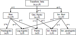
The beta-transformed family is based on the beta distribution of the second kind (or type II), that is, the distribution of X/(1—X) when X follows a beta distribution of type I, see the previous subsection. The beta distribution of type II has a density Renaming , the transformed beta is the distribution of and has the following density and distribution function :
where and denotes the incomplete lower beta function. These two families are available in actuar.
2.1.2 Discrete Distributions
The Sundt (a, b, 0) family of distributions is the set of distributions verifying
for and positive parameters. This recurrence equation can be seen a simplied discrete equation of the Pearson system (see Johnson et al. (2005)). We get back to the binomial distribution B(n, p) with ,and the Poisson distribution with and the negative binomial distribution N B(m, p) with . A generalization of the (a, b, 0) family is obtained by truncating the values smaller than n. Thus, the (a, b, n) family verifies
Furthermore, the exponential family also models discrete distributions by considering the mass probability function that verifies
It includes many familiar distributions: the Bernoulli distribution with d =1, a(x) = x, a(p) = log(p/(1 — p)), b(x) = 0 and , and the Poisson distribution with . See Chapter 14 for a discussion of the negative binomial distribution and the exponential family.
As for continuous distributions, discrete distributions are implemented in four functions: dfoo computes the mass probability function pxpfoo the cumulative distribution function Fx, qfoo the quantile function and rfoo the random number generator. For instance, the Poisson distribution is implemented in dpois, etc. Here is a standard call:
> dpois(0:2, lambda=3)
[1] 0.04978707 0.14936121 0.22404181
> ppois(1:2, lambda=3)
[1] 0.1991483 0.4231901
> qpois(1/2, lambda=3)
[1] 3
> rpois(5, lambda=3)
[1] 2 2 3 5 2
Typical transformations of an integer-valued random variable X are listed: (i) translation X + m for a non-null interger m (e.g. the shifted Poisson distribution), (ii) scaling mX, (iii) zero-inflation (1 — B)X where B follows a Bernoulli distribution B(q) and (iv) zero- modification (1 — B)(X + 1) where B follows a Bernoulli distribution. The resulting mass probability function for the transformed variable Y is
The zero-modification and the zero-inflation are useful to add a parameter to standard discrete distributions, for example, the Poisson distribution. A particular of the zero- modification is the zero-truncation when the variable B equals almost surely 0. Those transformations will be considered in Chapter 14, in the context of modeling claims frequency in motor insurance.
Such transformations are implemented in special packages, see the task view, but can be easily implemented.
> dpoisZM <- function(x, prob, lambda)
+ prob*(x == 0) + (1-prob)*(x > 0)*dpois(x-1, lambda)
> ppoisZM <- function(q, prob, lambda)
+ prob*(q >= 0) + (1-prob)*(q > 0)*ppois(q-1, lambda)
> qpoisZM <- function(p, prob, lambda)
+ ifelse(p <= prob, 0, 1+qpois((p-prob)/(1-prob), lambda))
> rpoisZM <- function(n, prob, lambda)
+ (1-rbinom(n, 1, prob))*(rpois(n, lambda)+1)
> x <- rpoisZM(100, 1/2, 3)
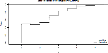
> plot(ecdf(x), main="Zero-modified Poisson(prob=1/2, lam=3)")
> lines(z <- sort(c(0:12, 0:12-1e-6)),
+ ppoisZM(z, 1/2, 3), col="grey", lty=4, lwd=2)
> legend("bottomright", lty=c(1,4), lwd=1:2,
+ col=c("black","grey"), leg=c("empir.","theo."))
In Figure 2.5, we plot the empirical cumulative distribution function of a zero-modified Poisson distribution.
The main discrete distributions are the binomial B(n,p), the Poisson P() and the negative binomial N B(m,p) distributions, for which we recall the mass probability function
for (the Bernoulli distribution is obtained with n =1).
for and
for . The discrete analog of the Pareto distribution is the Zipf distribution whose mass probability function is given by
where ζ(.) is the zeta’s Rieman function; see Olver et al. (2010).
2.1.3 Mixed-Type Distributions
Mixed-type distributions are distributions of random variables that are neither continuous nor discrete, that is, the set of discontinuities where the lower bound corresponds to continuous distributions and the upper bound discrete distributions. Thus, the distribution function has discontinuities and continuous parts. A first example of mixed-type distribution is the zero-modified gamma distribution which has the distribution function
where denotes the incomplete gamma function. X has an improper density function . In a similar way, zero-modified Pareto or zero-modified lognormal distributions can be defined.
An application of mixed-type distributions to destruction rate models is now presented. Destruction rate models focus on the distribution X = L/d where L is the loss amount and d the maximum possible loss (as defined in the insurance terms). By definition, X is bounded to the interval [0,1], and may have a mass at 1 when the object insured is entirely destroyed. In the application that will follow, we will consider the one-modified beta and the MBBEFD distributions. The one-modified beta is the distribution of X = BY where Y follows a beta distribution B(a, b) and B follows a Bernoulli distribution B(q). The distribution function is given by
for which the improper density is In R, we define it as
> dbetaOM <- function(x, prob, a, b)
+ dbeta(x, a, b)*(1-prob)*(x != 1) + prob*(x == 1)
> pbetaOM <- function(q, prob, a, b)
+ pbeta(q, a, b)*(1-prob) + prob*(q >= 1)
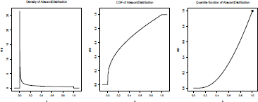
The Maxwell-Boltzmann Bore-Einstein Fermi-Dirac (MBBEFD) distribution was introduced and popularized by Bernegger (1997) in the context of reinsurance treaties. The distribution function is given by
where Note that there is a probability
mass at 1, since ℙ(X=1)=(a+1)b/(a+b)=qThe improper density function is
At the time this book is written, there is no package implementing the MBBEFD distribution,
but this can be remedied by the following lines:
> dMBBEFD <- function(x, a, b)
+ -a*(a+1)*b"x*log(b)/(a + b"x)"2 + (a+1)*b/(a+b)*(x == 1)
> pMBBEFD <- function(x, a, b)
+ a*((a+1)/(a+b"x)-1)*(x<1)+1*(x>=1)
Those two distributions will be used in the subsequent section on destruction rate data.
Mixing distributions consists of randomly drawing a distribution among a finite set of distributions. Consider a set of distribution functions and a set of weights . The choice of a distribution is such that . The random generation process given by (i) draw according to and (ii) draw according to Fc knowing is the mixture distribution among according to . This is characterized by the following distribution function
for all . If distributions are differentiable, then the density function of the mixture variable X is simply
A first simple example is the mixture of two normal distributions with the following density:
with a proportion This distribution is implemented in the package mixtools and norm1mix. A second example of more interest in actuarial science is the mixture of a light-tailed and heavy-tailed claim distribution. Say, for example, the mixture of a gamma distribution and a Pareto distribution . The density is given by
with a proportion . In R, we implement it as
> library(actuar)
> dmixgampar <- function(x, prob, nu, lambda, alpha, theta)
+ prob*dgamma(x, nu, lambda) + (1-prob)*dpareto(x, alpha, theta)
> pmixgampar <- function(q, prob, nu, lambda, alpha, theta)
+ prob*pgamma(q, nu, lambda) + (1-prob)*ppareto(q, alpha, theta)
where dpareto is implemented in the actuar package.
Another important family obtained using mixtures are the so-called phase-type distributions, obtained as mixtures of exponential distributions. Given p a vector of probabilities of length k, and matrix, X is said to be phase-type distributed, with parameters p and M if
where exp denotes here the matrix exponential; see Moler & Van Loan (1978) for a recent survey. The phase-type distribution can be seen as the distribution of the time to absorption (in the state 0) of a Markov jump process on the set {0,1,... ,n} with initial probability (0, p) and intensity matrix
![]()
where the vector . Observe that X has density
In package actuar, phtype distributions do exist, prob being vector p and rates being matrix M. One particular case is the Erlang distribution: Erlang (k, ) distribution, with density
is obtained when p = (1,0,..., 0) (of length k), and M is the matrix with — on the diagonal, A above, and elsewhere (seeO’Cinneide (1990) and Bladt (2005) for more details). To generate an Erlang distribution with k = 3 and = 2, one can use
> M <- matrix(0,3,3)
> diag(M) <- -2
2
> diag(M[1:(nrow(M)-1),2:ncol(M)])
> M
[,1] [,2] [,3]
[1,] -2 2 0
[2,] 0 -2 2
[3,] 0 0 -2
> set.seed(123)
> rphtype(5, prob=c(1,0,0), rates=M)
[1] 0.3311529 2.3017693 0.5631011 2.7375481 2.0612129
Other distributions such as mixture of generalized Erlang distributions are phase-type, but it is shown that a phase-type distribution does have Laplace transform . Therefore, the phase-type family does not include heavy-tailed distribution.
2.1.4 S3 versus S4 Types for Distribution
In the previous chapter, the distinction between S3 and S4 objects was introduced. Some packages allow one to use S4 objects to deal with distributions. For instance, using
> library(distr)
> library(distrEx)
we define an object, which is a distribution, and then various functions can be used to get the density, the quantile function or a random number generator, based on that distribution. Consider, for instance, the N(5, 22) distribution:
> X <- Norm(mean=5,sd=2)
> X
Distribution Object of Class: Norm
 mean: 5
 sd: 2
If we want to compute quantiles associated to that distribution, we use the quantile q() function: q(X) is then the function ,
> q(X)
function (p, lower.tail = TRUE, log.p = FALSE)
{
qnorm(p, mean =5, sd = 2, lower.tail = lower.tail, log.p = log.p)
}
<environment: 0x10d796c98>
And if we want to evaluate that function, for instance to get the value of , we use
> q(X)(0.25)
[1] 3.65102
(which is the same as the standard qnorm(0.25,mean=5,sd=2)). Various functions can also be used to derive simple quantities associated to that distribution, such as moments
> mean(X)
[1] 5
We can also create discrete distributions, such as
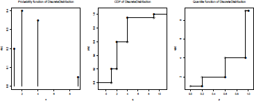
> N <- DiscreteDistribution(supp=c(1,2,4,9) , prob=c(.2,.4,.35,.05))
where the support supp and the associate probabilities prob are mentioned. One can then use r() to generate random numbers, d() to compute the density function, p() to compute the cumulative distribution function, and q() to compute the quantile function. We can also visualize that distribution using
> plot(N)
An interesting feature of this S4 class is that simple arithmetics on distributions can be performed. Consider two distributions X1 and X2:
> X1 <- Norm(mean=5,sd=2)
> X2 <- Norm(mean=2,sd=1)
then operator + can be used to define a distribution which will be the sum of two independent Gaussian random variables,
> S <- X1+X2
> plot(S)
If we look at the titles on Figure 2.7, we can see that S is recognized as a Gaussian distribution (the sum of two independent Gaussian distributions being also a Gaussian distribution).
Other operators can be used, such as -, * or /, even ^,
> U <- Unif(Min=0,Max=1)
> N <- DiscreteDistribution(supp=c(1,2,4,9), prob=c(.2,.4,.35,.05))
> Z <- U"N
> plot(Z)
Such a function is (absolutely continuous), and is recognized as an AbscontDistribution object. A more complex object is obtained if N can take value 0. Then, the distribution is no longer absolutely continuous:
> N <- DiscreteDistribution(supp=c(0,1,2,4) , prob=c(.2,.4,.35,.05))
> Z <- U~N
> Z
An object of class "UnivarLebDecDistribution"
--- a Lebesgue decomposed distribution:
Its discrete part (with weight 0.200000) is a Distribution Object of Class: Dirac location: 1
This part is accessible with ’discretePart(<obj>)’.
Its absolutely continuous part (with weight 0.800000) is a Distribution Object of Class: AbscontDistribution This part is accessible with ’acPart(<obj>)’.
Using plot(Z), we can see that this distribution has two components: a (absolutely) continuous one, and a Dirac mass, in 1.
Observe finally that compound distributions can also be generated easily. The standard compound Poisson distribution is obtained using
> CP <- CompoundDistribution(Pois(), Gammad())
> CP
An object of class "CompoundDistribution"
The frequency distribution is:
Distribution Object of Class: Pois lambda: 1
The summands distribution is/are:
Distribution Object of Class: Gammad
shape: 1
scale: 1
2.2 Parametric Inference
Parametric inference deals with the estimation of an unknown parameter of a chosen distribution. The experimenter assumes that are realizations of a random sample such that X are independent and identically distributed randoms variables according to a generic random variable X (this is the blanket assumption). The random variable X has a distribution function F(.; )for . For example, when considering an exponential distribution . In the following subsequent sections, classical estimation methods are presented and provide criteria to establish an estimator of . Once a model is fitted, the experimenter can derive its quantities of interest (mean, variance, quantiles, survival probabilities,. . .), derived from the fitted distribution . In most applications, X has either a continuous or a discrete distribution. Therefore, we work either the density function or the mass probability function . For a general introduction to statistical inference, we refer to Casella & Berger (2002).
2.2.1 Maximum Likelihood Estimation
As its name suggests, maximum likelihood estimation consists of maximizing the likelihood with respect to , which is defined as
depending on the type of the random variable X. For many reasons, it is more convenient to maximize the log-likelihood log L with respect to A school example is to consider the exponential distribution , that is, . The maximizer is leading to the estimator . In practice, closed-form formulas of the maximizers may not exist, thus we use a numeric optimization. The fitdistrplus package provides routines to compute the maximum likelihood estimator for most standard distributions.
We consider a claim dataset itamtplcost which contains large losses (in excess of 500,00 euros) of an Italian Motor-TPL company since 1997. For pedagogical purposes (despite that the distribution is not really appropriate), we choose to fit a gamma distribution defined as , with parameter
> data(itamtplcost)
> library(fitdistrplus)
> x <- itamtplcost$UltimateCost / 10"6
> summary(x)
Min. 1st Qu. Median Mean 3rd Qu. Max.
0.002161 0.627700 0.844000 1.015000 1.224000 6.639000
> fgamMLE <- fitdist(x, "gamma", method="mle")
> fgamMLE
Fitting of the distribution ' gamma ' by maximum likelihood Parameters:
estimate Std. Error
shape 2.398655 0.1489696
rate 2.362486 0.1631542
> summary(fgamMLE)
Fitting of the distribution ' gamma ' by maximum likelihood
Parameters :
estimate Std. Error
shape 2.398655 0.1489696
rate 2.362486 0.1631542
Loglikelihood: -385.1474 AIC: 774.2947 BIC: 782.5441
Correlation matrix:
shap rate
shape 1.0000000 0.8992915
rate 0.8992915 1.0000000
Without a scaling of cost from euros to millions of euros, the call to fitdist raises an error, thus we divide the ultimate cost by 106. In this example, is estimated as (2.398655, 2.362486). Note that the fitdist function returns an S3-object of class fitdist, for which print, summary and plot methods have been defined. In addition to the estimation of standard errors of , the summary method gives an estimation of the asymptotic correlation matrix as well as the (optimal) log-likelihood. This is based on the asymptotic normality of the maximum likelihood estimators (under the hypotheses of the Cramer-Rao model; see Casella & Berger (2002)).
2.2.2 Moment Matching Estimation
The moment matching estimation is also commonly used to fit parametric distributions. This consists of finding the value of the parameter that matches the first theoretical raw moments of the parametric distribution to the corresponding empirical raw moments as
for k = 1,... ,d, with d the number of parameters to estimate and the n observations of variable X. For moments of order greater than or equal to 2, it may be relevant to match centered moments defined as
where denotes the empirical centered moments. For instance, consider the gamma distribution . The moment matching estimation solves
In general, there are no closed-form formulas for this estimator and use a numerical method. Still considering the gamma distribution fit on the MTPL dataset, we use the fitdistrplus package.
> fgamMME <- fitdist(x, "gamma", method="mme")
> cbind(MLE=fgamMLE$estimate, MME=fgamMME$estimate)
MLE MME
shape 2.398655 2.229563
rate 2.362486 2.195851
2.2.3 Quantile Matching Estimation
Fitting of a parametric distribution may also be done by matching theoretical quantiles of the parametric distribution (for some specified probabilities) against the empirical quantiles (see Tse (2009) among others). The equation below is very similar to the previous equations for matching moments
for the empirical quantiles for specified probabilities pk. Empirical quantiles are computed on observations using the quantile function of the stats package. When is an integer, the empirical quantile is uniquely defined as , where is the sorted sample. Otherwise, the empirical quantile is the convex combination of see ?quantile and Hyndman & Fan (1996). The theoretical quantile F-1(.; ) can have a closed-form formula. For example, when considering the exponential distribution , the quantile function is
Solving the d equations is achieved by a numeric optimization in the fitdist function.
Continuing the MTPL example, we fit a gamma distribution against the probabilities
> fgamQME <- fitdist(x, "gamma", method="qme", probs=c(1/3, 2/3))
> cbind(MLE=fgamMLE$estimate, MME=fgamMME$estimate,
+ QME=fgamQME$estimate)
MLE MME QME
shape 2.398655 2.229563 4.64246
rate 2.362486 2.195851 4.95115
Note that compared to the method of moments and the maximum likelihood estimation, the estimate paramater differs significantly when using the quantile matching estimation, despite considering probabilities in the heart of the distribution.
2.2.4 Maximum Goodness-of-Fit Estimation
A last method of estimation called maximum goodness-of-fit estimation or (minimum distance estimation) is presented here; see D’Agostino & Stephens (1986) or Dutang et al. (2008) for more details. In this section, we focus on the Cramer-von Mises distance and refer to Delignette-Muller & Dutang (2013) for other distances (i.e. Kolmogorov-Smirnov and Anderson-Darling). The Cramer-von Mises looks at the squared difference between the candidate distribution and the empirical distribution function Fn, the latter being defined as the percentage of observations below x: . The Cramer-von Mises distance is defined as
and is estimated in practice by
The maximum goodness-of-fit estimation consists of finding the value of minimizing . The name comes from the fact that the Cramer-von Mises distance measures the goodness- of-fit of F(.; ) against . There is no closed-form formula for argmin , and a numerical optimization is used in the fitdist function.
Finally, we fit a gamma distribution by maximum goodness-of-fit estimation:
> fgamMGE <- fitdist(x, "gamma", method="mge", gof="CvM")
> cbind(MLE=fgamMLE$estimate, MME=fgamMME$estimate,
+ QME=fgamQME$estimate, MGE=fgamMGE$estimate)
MLE MME QME MGE
shape 2.398655 2.229563 4.64246 3.720546
rate 2.362486 2.195851 4.95115 3.875971
As for quantile matching estimation, the value of differs widely. A practitioner approach could be take the average by component irrespectively of the methods tested. This leads to the question of how to choose between fitted parameters and between fitted distributions.
2.3 Measures of Adequacy
This section focuses on measures of adequacy either graphical methods or numerical methods.
2.3.1 Histogram and Empirical Densities
A typical plot to assess the adequacy of a distribution is the histogram. We recall that for plotting a histogram, observed data are divided into k classes (generally k is proportional to log(n)); the number of observation in each class is computed, that is, frequencies ; finally rectangles are drawn such that the basis is a class and the height is the absolute or the relative frequencies. Thus, the histogram is an estimator of the empirical density, as the area of a rectangle is proportional to . This graph is generically provided in the plot function of a fitdist object, but does not allow multiple fitted distributions. So in the example of a gamma fit to the MTPL dataset, we use the denscomp function:
> txt <- c("MLE","MME","QME(1/3, 2/3)", "MGE-CvM")
> denscomp(list(fgamMLE, fgamMME, fgamQME, fgamMGE), legendtext=txt,
+ fitcol="black", main="Histogram and fitted gamma densities")
Alternatively, we can estimate directly the density function by the popular kernel density estimation. This is implemented in the density function as shown below
> hist(x, prob=TRUE, ylim=c(0, 1))
> lines(density(x), lty=5)
In order to better assess the fitted gamma densities, the two above graphs are plotted on separate graphics. We observe that the MLE and the MME fits best approximates the density between , while the QME and the MGE fit best assess the density between . However, it is clear that the gamma distribution cannot appropriately fit the whole distribution, mainly due to its light-tailedness.
2.3.2 Distribution Function Plot
Another typical graph is to plot the fitted distribution and the empirical cumulative distribution function . As already given, the computation of is simpler than for the empirical density . A new claim dataset is considered to illustrate this type of plot: we use the popular Danish dataset, used in McNeil (1997). The dataset is stored in danishuni for the univariate version and contains fire loss amounts collected at Copenhagen Reinsurance between 1980 and 1990. We consider three distributions: a gamma distribution
a Pareto distribution a Pareto-gamma mixture defined in Section 2.1.3 and a Burr distribution
> data(danishuni)
> x <- danishuni$Loss
> fgam <- fitdist(x, "gamma", lower=0)
> fpar <- fitdist(x, "pareto", start=list(shape=2, scale=2), lower=0)
> fmixgampar <- fitdist(x, "mixgampar", start=
+ list(prob=1/2, nu=1, lambda=1, alpha=2, theta=2), lower=0)
> cbind(SINGLE= c(NA, fgam$estimate, fpar$estimate),
+ MIXTURE=fmixgampar$estimate)
SINGLE MIXTURE
NA 0.6849568
shape 1.2976150 10.8706430
rate 0.3833335 6.5436349
shape 5.3689277 5.4182746
scale 13.8413207 30.0700544
When fitted alone, the parameters of the gamma distribution are estimated as (1.2976, 0.3833) and the parameters of the Pareto distribution are estimated as (5.3689,13.8413). When used in the mixture, we get
As only the shape parameter is of similar amplitude, only heavy-tailed distributions (like the Pareto) are appropriate for this dataset. Finally, we fit a Burr distribution:
> fburr <- fitdist(x, "burr", start=list(shape1=2, shape2=2,
+ scale=2), lower=c(0.1,1/2, 0))
> fburr$estimate
shape1 shape2 scale
0.10000 14.44286 1.08527
Comparing the fitted densities is then carried out using the cdfcomp function:
> cdfcomp(list(fgam, fpar, fmixgampar, fburr), xlogscale=TRUE,
+ datapch=".", datacol="grey", fitcol="black", fitlty=2:5,
+ legendtext=c("gamma","Pareto","Par-gam","Burr"),
+ main="Fitted CDFs on danish")
We also plot the tail of the distribution function on Figure 2.10 When using the maximum likelihood estimation, the best fit is provided by the Burr distribution, yet the first shape parameter hits the lower bound of 0.1.


2.3.3 QQ-Plot, PP-Plot
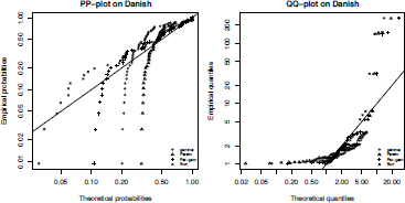
On the two previous graphs, we consider the plot of the empirical density (respectively the empirical distribution function) and the fitted density (respectively the fitted distribution function). The PP-plot (respectively the QQ-plot) consists of plotting (directly) the empirical distribution function against the fitted distribution function (respectively the empirical quantile function against the fitted quantile function Those quantities are computed at the observations, which leads to further simplifications This is illustrated on the Danish fire dataset danishuni and the four distributions considered by using the ppcomp and qqcomp functions:
> qmixgampar <- function(p, prob, nu, lambda, alpha, theta)
+ {
+ L2 <- function(q, p)
+ (p - pmixgampar(q, prob, nu, lambda, alpha, theta))"2 + sapply(p, function(p) optimize(L2, c(0, 10"3), p=p)$minimum)
+}
> ppcomp(list(fgam, fpar, fmixgampar, fburr), xlogscale=TRUE,
+ ylogscale=TRUE, fitcol="black", main="PP-plot on danish",
+ legendtext=c("gamma","Pareto","Par-gam","Burr"), fitpch=1:4)
> qqcomp(list(fgam, fpar, fmixgampar, fburr), xlogscale=TRUE,
+ ylogscale=TRUE, fitcol="black", main="QQ-plot on danish",
+ legendtext=c("gamma","Pareto","Par-gam","Burr"), fitpch=1:4)
As there is no closed-form formula for the quantile function of the mixture distribution (i.e. inverse of a numerical optimization is carried out using the Golden line-search (implemented in optimize). On Figure 2.11, quantiles and probabilities are plotted as a point, while the straight line corresponds to the identity function. The more points that are close to the line, the better fit the distribution. The pp-plot reveals that only the Burr distribution sufficiently fits the data, whereas the qq-plot shows that both the Pareto-gamma mixture and the Burr distributions best approximate the data.
The plot method of a fitdist object provides the four above graphs (for the fitted distribution) in the following order: a histogram with the fitted density, an ecdf-plot with the fitted distribution function, a (theoretical) quantile—(empirical) quantile plot and a (theoretical) probability—(empirical) probability plot.
2.3.4 Goodness-of-Fit Statistics and Tests
We turn our attention to goodness-of-fit statistics to complement the four previous goodness- of-fit graphs. For continuous distributions, the three statistics presented in Section 2.2.4 can be computed, that is, Cramer-von Mises, Kolmogorov-Smirnov and Anderson-Darling statistics. For discrete distributions, the more common statistic is the chi-square statistic defined as
where is the empirical frequency count for the level i, n is the total number of observations, the theoretical probability (i.e. the theoretical frequency count), and m is the number of cells. In practice, the number of cells is either fixed by the experimenter or chosen so that empirical frequencies are greater than five and is replaced by . The chi-square statistic is linked to the Pearson’s hypothesis test of goodness- of-fit, for which under the null hypothesis, converges in law to a chi-square distribution (m — d — 1) (where d is the number of parameters). For all distributions, we consider also the information criteria (AIC and BIC) proportional to the opposite of the log-likelihood. All of this is provided in the gofstat function (of the fitdistrplus package). A numerical illustration is proposed on a TPL claim number dataset, for which a Poisson, a negative binomial and a zero-modified Poisson distribution are fitted using maximum likelihood techniques.
> data(tplclaimnumber)
> x <- tplclaimnumber$claim.number
> fpois <- fitdist(x, "pois")
> fnbinom <- fitdist(x, "nbinom")
> fpoisZM <- fitdist(x, "poisZM", start=list(
+ prob=sum(x == 0)/length(x), lambda=mean(x)),
+ lower=c(0,0), upper=c(1, Inf))
> gofstat(list(fpois, fnbinom, fpoisZM), chisqbreaks=c(0:4, 9),
+ discrete=TRUE, fitnames=c("Poisson","NegBinomial","ZM-Poisson"))
Chi-squared statistic: Inf 11765679 Inf
Degree of freedom of the Chi-squared distribution: 5 4 4
Chi-squared p-value: 0 0 0
the p-value may be wrong with some theoretical counts < 5
Chi-squared table:
obscounts theo Poisson theo NegBinomial theo ZM-Poisson
<=0 653047 6.520559e+05 6.530606e+05 6.530411e+05
<= 1 23592 2.545374e+04 2.353633e+04 2.351466e+04
<= 2 1299 4.968076e+02 1.326372e+03 1.413873e+03
<= 3 62 6.464481e+00 8.372804e+01 4.250619e+01
<= 4 5 6.308707e-02 5.568862e+00 8.519276e-01
<= 9 5 4.957574e-04 4.104209e-01 1.296158e-02
> 9 3 0.000000e+00 7.649401e-07 0.000000e+00
Goodness-of-fit criteria
Poisson NegBinomial ZM-Poisson
Aikake's Information Criterion 226880.4 225375.1 225585.7
Bayesian Information Criterion 226891.8 225398.0 225608.5
From the chi-square statistic and the chi-square table the negative binomial distribution is clearly the best distribution. This is also confirmed by the AIC and the BIC criteria.
2.3.5 Skewness—Kurtosis Graph
When selecting a distribution, depending on the type of applications, the experimenter may give particular attention to the tail, some quantiles or the body of the distribution for which a natural way of choosing the “best” distribution emerges. In actuarial science, a great care is given to the tail of distribution, and also on first moments. The code below provide values of quantiles (plotted before) as well as the first two raw moments.
> p <- c(.9, .95, .975, .99)
> rbind(
+ empirical= quantile(danishuni$Loss, prob=p),
+ gamma= quantile(fgam, prob=p)$quantiles,
+ Pareto= quantile(fpar, prob=p)$quantiles,
+ Pareto_gamma= quantile(fmixgampar, prob=p)$quantiles,
+ Burr= quantile(fburr, prob=p)$quantiles)
p=0.9 p=0.95 p=0.975 p=0.99
empirical 5.541526 9.972647 16.26821 26.04253
gamma 7.308954 9.261227 11.18907 13.71207
Pareto 7.412375 10.341301 13.67386 18.79426
Pareto_gamma 7.093200 12.164896 17.92871 26.77259
Burr 5.344677 8.636739 13.95655 26.32118
> compmom <- function(order)
+ c(empirical= sum(danishuni$Loss"order)/length(x),
+ gamma=mgamma(order, fgam[[1]][1], fgam[[1]][2]),
+ Pareto=mpareto(order, fpar[[1]][1], fpar[[1]][2]),
+ Pareto_gamma= as.numeric(fmixgampar[[1]][1]*
+ mgamma(order, fmixgampar[[1]][2], fmixgampar[[1]][3]) +
+ (1-fmixgampar[[1]][1])*
+ mpareto(order, fmixgampar[[1]][4], fmixgampar$estimate[5])),
+ Burr=mburr(order, fburr[[1]][1], fburr[[1]][2], fburr[[1]][3]))
> rbind(Mean=compmom(1), Mom2nd= compmom(2))
empirical gamma Pareto Pareto_gamma Burr
Mean 0.01081909 3.385081 3.168128 3.28202 2.98562
Mom2nd 0.26784042 20.289412 26.032657 39.78745 Inf
For higher moments, it is typical to look at the skewness and the kurtosis coefficients defined as
for a random variable X. For heavy-tailed distributions, such coefficients may not exist, yet empirically they always exist. The descdist function provides the so-called Cullen and Frey graph, which plots the empirical estimates of sk(X) and kr(X) as well as the possible values for some classic distributions (including the gamma family for continuous distributions and the Poisson distribution for discrete distributions) This is illustrated on the danishuni and the tplcaimnumber datasets on Figure 2.12, using so-called Cullen and Frey graphs, from Cullen & Frey (1999). The fit analysis can also be completed by looking at the uncertainty of parameter estimate with a bootstrap analysis. This is possible with the bootdist function of fitdistrplus.

Cullen and Frey graph for danish and tplclaimnumber, on the left and on the right, respectively.
2.4 Linear Regression: Introducing Covariates in Statistical Inference
In the first part of this chapter, we did mention the normal distribution. If it is still a popular distribution in financial models (see Chapter 11), it is also frequently used in actuarial science because of its connection with linear regression.
2.4.1 Using Covariates in the Statistical Framework
So far, we have assumed that observations were i.i.d., for example, with distribution . But in most assumptions, it can yield a very restrictive model. For instance, consider dataset Davis and let X denote the height of a person (in centimeter):
> X <- Davis$height
We can fit a Gaussian distribution to the weight
> (param <- fitdistr(X,"normal")$estimate)
mean sd
170.56500 8.90987
If we plot the distribution (see Figure 2.13), we can see that using a mixture of two Gaussian distributions is much better than using only a single model,
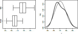
Distribution of the height, using a normal distribution, and mixtures of normal distributions: One with a non-observable latent factor, one where mixture is related to the sex.
(where the + sign should be understood in the context of mixtures, as described in Section 2.1.3). This model can be estimated using maximum likelihood techniques. Let us define the log-density as
> logdf <- function(x,parameter){
+ p <- parameter[1]
+ ml <- parameter[2]
+ sl <- parameter[4]
+ m2 <- parameter[3]
+ s2 <- parameter[5]
+ return(log(p*dnorm(x,m1,s1)+(1-p)*dnorm(x,m2,s2)))
+}
and in order to take into account various constraints, namely that can be written
Function constrOptim will seek the minimum of a function, so we will consider here the opposite of the log-likelihood:
> logL <- function(parameter) -sum(logdf(X,parameter))
> Amat <- matrix(c(1,-1,0,0,0,0,
+ 0,0,0,0,1,0,0,0,0,0,0,0,0,1), 4, 5)
> bvec <- c(0,-1,0,0)
> constr0ptim(c(.5,160,180,10,10), logL, NULL, ui = Amat, ci = bvec)$par [1] 0.5996263 165.2690084 178.4991624 5.9447675 6.3564746
Because we use a (finite) normal mixture here, it is also possible to use the EM algorithm, from the mixtools package,
> library(mixtools)
> mix <- normalmixEM(X) number of iterations= 391
> (param12 <- c(mix$lambda[1],mix$mu,mix$sigma))
[1] 0.5995197 165.2676186 178.4951348 5.9448806 6.3579494
The two methods yield rather similar outputs.
If previously we assumed that the mixing variable 0 was a latent unobservable random variable, here it would make sense to assume that a good proxy of this variable can be the sex of the individuals. And here,
Here, and are known, and are, respectively, the proportion of males and females in the population.
> sex <- Davis$sex
> (pM <- mean(sex=="M"))
[1] 0.44
> (paramF <- fitdistr(X[sex=="F"],"normal")$estimate)
mean sd
164.714286 5.633808
> (paramM <- fitdistr(X[sex=="M"],"normal")$estimate)
mean sd
178.011364 6.404001
If we compare the three models, including a kernel-based estimator, we obtain the graph of Figure 2.13.
> f1 <- function(x) dnorm(x,param[1],param[2])
> f2 <- function(x) param12[1]*dnorm(x,param12[2],param12[4]) +
+ (1-param12[1])*dnorm(x,param12[3],param12[5])
> f3 <- function(x) pM*dnorm(x,paramM[1],paramM[2]) + (1-pM)*dnorm(x,paramF[1],paramF[2])
> boxplot(X~sex,horizontal=TRUE,names=c("Female","Male"))
> x <- seq(min(X),max(X),by=.1)
> plot(x,f1(x),lty=2,type="l")
> lines(x,f2(x),col="grey",lwd=2)
> lines(x,f3(x),col="black",lwd=2)
> lines(density(X))
Actually, this factor-based mixture is a particular case of what is known as the linear model.
2.4.2 Linear Regression Model
To use standard notions in regression modeling, let Y denote the variable of interest. And assume that some additional variables can be used, denoted . This means that for each observation , we observe also . As discussed in Chapter 14, ’s can be either numeric (also called continuous) or categorical (also called factor) variables.
In the Davis dataset, the varible of interest is the height of a person, denoted height (our variable Y), and two additional variables can be used, sex (variable ) and weight (variable ).
> Y <- Davis$height
> X1 <- Davis$sex
> X2 <- Davis$weight
> df <- data.frame(Y,X1,X2)
Instead of assuming that
,
we will assume, in a regression model, that
where is now a function of the explanatory variables. Consider here the case where we observe two covariates, the sex and the weight (in kilograms) of the individuals. If we restrict ourselves to linear models, then
From properties of the Gaussian distribution, it is also possible to write this model as
where ε is an error term, usually called residuals, centered, and normally distributed,
The unknown parameters (that should be estimated) are now
2.4.3 Inference in a Linear Model
Recall, first of all, that the previous model cannot be identified: We cannot have the intercept and the two factors (M and F) at the same time. The standard procedure is to keep the intercept and to remove one of the two factors. The factor that was dropped will become the reference.
The maximum likelihood estimator is obtained by maximizing
where here is the density of the distribution.
Here, the maximum likelihood estimators of the set of parameters can be written explicitly. When writing the problem using the logarithm of the likelihood, we can observe that the optimal value of = should satisfy
Thus, using maximum likelihood techniques in a Gaussian linear model is the same as minimizing the sum of squares of residuals (known as Ordinary Least Squares estimation).
Fitting a linear model is done using function lm(). Using symbolic notions (introduced in Chapter 1), we write here
> lin.mod <- lm(Y~X1+X2,data=df)
As mentioned in Chapter 1, lin.mod is a S3 object, and many functions can be used to extract information from that object. To visualize the standard output of a linear regression, use
> summary(lin.mod)
Call:
lm(formula = Y ~ X1 + X2, data = df)
Residuals:
Min 1Q Median 3Q Max
-85.204 -4.183 0.446 5.224 19.009
Coefficients:
Estimate Std. Error t value Pr(>|t|)
(Intercept) 175.26607 3.30681 53.002 < 2e-16 ***
X1M 17.86160 1.66941 10.699 < 2e-16 ***
X2 -0.19917 0.05503 -3.619 0.000376 ***
---
Signif. codes: 0 *** 0.001 ** 0.01 * 0.05 . 0.1 1
Residual standard error: 9.424 on 197 degrees of freedom
Multiple R-squared: 0.3903, Adjusted R-squared: 0.3841
F-statistic: 63.05 on 2 and 197 DF, p-value: < 2.2e-16
It is also possible to get predictions, using predict. Keep in mind that we should have the same input format as in the lm call: The regression was run on a dataframe, so predict should also be called on a dataframe (with the same variable names),
> new.obs <- data.frame(X1=c("M","M","F"),X2=c(100,70,65))
> predict(lin.mod,newdata=new.obs)
1 2 3
173.2110 179.1860 162.3202
which will return for any observation x.
Linear models with R have been intensively described, so we refer to Venables & Ripley (2002), Fox & Weisberg (2011) or Kleiber & Zeileis (2008) for more details. Extensions of this model will be given in the next chapters (the logistic regression of binary responses in Chapter 4, and GLMs in Chapter 14, among others) as well as a Bayesian interpretation of this model (in Chapter 3).
2.5 Aggregate Loss Distribution
This section deals with the aggregate loss amount distribution, which is the distribution of the compound sum
where N is the claim number and ()’s are the claim severities (which are assumed to be strictly positive). Firstly, the computation of the distribution function of S is studied. Then, an application to a TPL motor dataset is carried out. Finally, a continuous-time version of this problem is analyzed via the ruin theory framework.
2.5.1 Computation of the Aggregate Loss Distribution
A classical assumption on the aggregate amount S is to require that N is independent of claim amounts . Another common assumption is that . Therefore, the distribution function simplifies to
where is the n-order convolution product of . In a small number of distributions of X, the distribution of the sum is easy. For instance, when X follows a gamma distribution, then the sum follows a gamma distribution . This can be implemented as
> pgamsum <- function(x, dfreq, argfreq, shape, rate, Nmax=10)
+ {
+ tol <- 1e-10; maxit <- 10 + nbclaim <- 0:Nmax
+ dnbclaim <- do.call(dfreq, c(list(x=nbclaim), argfreq))
+ psumfornbclaim <- sapply(nbclaim, function(n)
+ pgamma(x, shape=shape*n, rate=rate))
+ psumtot <- psumfornbclaim dnbclaim + dnbclaimtot <- dnbclaim + iter <- 0
+ while(abs(sum(dnbclaimtot)-1) > tol && iter < maxit)
+ {
+ nbclaim <- nbclaim+Nmax
+ dnbclaim <- do.call(dfreq, c(list(x=nbclaim), argfreq))
+ psumfornbclaim <- sapply(nbclaim, function(n)
+ pgamma(x, shape=shape*n, rate=rate))
+ psumtot <- psumtot + psumfornbclaim dnbclaim
+ dnbclaimtot <- c(dnbclaimtot, dnbclaim)
+ iter <- iter+1
+}
+ as.numeric(psumtot)
+}
In general, the distribution of the sum does not necessarily have the same distribution as X. Alternative computations are possible. The Panjer recursion provides a recursive method to compute the mass probability function of S in the case that X has a discrete distribution and N belongs to the (a, b, n) family; see Panjer (1981). The recursion formula for the mass probability function is
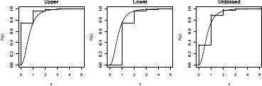
Where has a discrete distribution on {0,1,…,m} with a mass probability function , N belongs to (a, b, 0) family and starting at the probability generating function. The recursion is stopped when the sum of elementary probabilities P(S = 0,1,...) is arbitrarily close to 1. In practice, the distribution of the claim amount is not discrete but can be discretized. The upper discretization is the forward difference
, the lower discretization is the backward difference and the unbiased discretization is , where h is the step of discretization; see Figure 2.14 and Dutang et al. (2008) for further details.
Approximations based on the normal distribution are also available: (i) the normal approximation is given by
(ii) the normal-power approximation is given by
,
where is the standard deviation of S and sk(S) is the skewness coefficient of S. The skewness coefficient can be written as
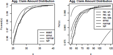
An approximation based on the gamma distribution is also possible; see Gendron & Crepeau (1989). These approximations are reasonably correct at the heart of the distribution but not at the tails of the distribution. A last alternative to exact computation is the simulation procedure. It consists of simulating n claim numbers , ’s claim severities in order to get n realizations . All these alternative methods are available in the aggregateDist function of the actuar package. We consider two examples: the gamma case (N follows a Poisson distribution P(10) and X follows a gamma distribution G(3, 2)) and the Pareto case (N follows a Poisson distribution P(10) and X follows a Pareto distribution P(3.1, 4.2)). The following code computes the gamma case:
> parsev <- c(3, 2); parfreq <- 10
> meansev <- mgamma(1, parsev[1], parsev[2])
> varsev <- mgamma(2, parsev[1], parsev[2]) - meansev"2
> skewsev <- (mgamma(3, parsev[1], parsev[2]) -
+ 3*meansev*varsev - meansev"3)/varsev"(3/2)
> meanfreq <- varfreq <- parfreq[1]; skewfreq <- 1/sqrt(parfreq[1])
> meanagg <- meanfreq * meansev
> varagg <- varfreq * (varsev + meansev"2)
> skewagg <- (skewfreq*varfreq"(3/2)*meansev"3 + 3*varfreq*meansev*
+ varsev + meanfreq*skewsev*varsev"(3/2))/varagg"(3/2)
> Fs.s <- aggregateDist("simulation", model.freq = expression(y =
+ rpois(parfreq)), model.sev = expression(y =
+ rgamma(parsev[1], parsev[2])), nb.simul = 1000)
> Fs.n <- aggregateDist("normal", moments = c(meanagg, varagg))
> Fs.np <- aggregateDist("npower", moments = c(meanagg, varagg, skewagg))
> Fs.exact <- function(x) pgamsum(x, dpois, list(lambda=parfreq),
+ parsev[1], parsev[2], Nmax=100)
> x <- seq(25, 40, length=101)
> plot(x, Fs.exact(x), type="l",
+ main="Agg. Claim Amount Distribution", ylab="F_S(x)")
> lines(x, Fs.s(x), lty=2)
> lines(x, Fs.n(x), lty=3)
> lines(x, Fs.np(x), lty=4)
> legend("bottomright", leg=c("exact", "simulation",
+ "normal approx.", "NP approx."), col = "black",
+ lty = 1:4, text.col = "black")
Similarly, we have the Pareto case. We show here only the recursive computation calls.
> parsev <- c(3.1, 2*2.1) ; parfreq <- 10
> xmax <- qpareto(1-1e-9, parsev[1], parsev[2])
> fx2 <- discretize(ppareto(x, parsev[1], parsev[2]), from = 0,
+ to = xmax, step = 0.5, method = "unbiased",
+ lev = levpareto(x, parsev[1], parsev[2]))
> Fs2 <- aggregateDist("recursive", model.freq = "poisson",
+ model.sev = fx2, lambda = parfreq, x.scale = 0.5, maxit=2000)
> fx.u2 <- discretize(ppareto(x, parsev[1], parsev[2]), from = 0,
+ to = xmax, step = 0.5, method = "upper")
> Fs.u2 <- aggregateDist("recursive", model.freq = "poisson",
+ model.sev = fx.u2, lambda = parfreq, x.scale = 0.5, maxit=2000)
> fx.l2 <- discretize(ppareto(x, parsev[1], parsev[2]), from = 0,
+ to = xmax, step = 0.5, method = "lower")
> Fs.l2 <- aggregateDist("recursive", model.freq = "poisson",
+ model.sev = fx.l2, lambda = parfreq, x.scale = 0.5, maxit=2000)
The two graphs are displayed on Figure 2.15. Despite the expectation that E(X) is identical in both cases, high-level quantiles of the aggregate claim distribution are significantly different. For the gamma case, the normal-power approximation suitably fits the exact distribution function, while for the Pareto case, the normal-power approximation overestimates as the skewness sk(S) is very high and not representative of the shape of the distribution. As their name suggests, the upper and the lower recursive computations surround the true distribution function. The simulation number is voluntarily chosen low (1,000), but can be set to a much larger number. If convergence is achieved for a high number of simulations, paral- lelization, GPU computation and quasi-Monte Carlo sampling methods can be used to fasten the process; see Chapter 1, http://cran.r-project.org/web/views/HighPerformanceComputing.html and http://cran.r-project.org/web/views/Distributions.html for more details.
2.5.2 Poisson Process
The Poisson process is probably the most important stochastic process in general insurance. It is used to describe the number of claims that occurred in a time interval. In its basic form, the homogeneous Poisson process is a counting process (), with independent and stationary increments. At time t, , the number of claims that occurred from time 0 until time t, has a Poisson distribution, and the distribution of waiting time until the next claim is an exponential distribution. Let () denote the ith arrival time, so that { = 0} can equivalently be represented by and more generally
In the case where interarrival times are i.i.d. random variables, then is called a renewal process, and it is fully characterized by the distribution of inter-arrival times, . The Poisson process is obtained when F is the distribution of an exponential random variable. The code to generate a renewal process up to time T, or more precisely an arrival time sequence, is
> rate <- 1
> rFexp <- function!) rexp(1,rate)
> rRenewal <- function(Tmax=1,rF=rFexp){
+ t <-0
+ vect.W<- NULL
+ while(t<Tmax){
+ W<-rF()
+ t<-t+W
+ if(t<T) vect.W=c(vect.W,W)}
+ return(list(T=cumsum(vect.W),W=vect.W,N=length(vW)))}
> set.seed(1)
> rRenewal(Tmax=2)
$T
[1] 0.7551818 1.9368246 $W
[1] 0.7551818 1.1816428
$N [1] 2
An interesting alternative, in the case of the Poisson process with intensity , is to use a uniform property of the process: For all , given {}, the joint distribution of the n arrival time is the same as the joint distribution of , the order statistics of n i.i.d. random variables uniformly distributed on [0,t]. Thus, a natural algorithm to generate the Poisson process is the following:
> rPoissonProc <- function(Tmax=1,lambda=rate){
+ N <- rpois(n=1,lambda*Tmax)
+ vect.T <- NULL
+ if(N>0) vect.T=sort(runif(N))*lambda*Tmax
+ return(list(T=vect.T,W=diff(c(0,vect.T)),N=N))}
> set.seed(1)
> rPoissonProc(T=5)
$T
[1] 1.008410 1.860619 2.864267 4.541039
$W
[1] 1.0084097 0.8522098 1.0036473 1.6767721
$N
[1] 4
An homogeneous Poisson process, with intensity satisfies
It is possible to consider a non-homogeneous Poisson process with intensity . Then
.
See Rolski et al. (1999) for more details.
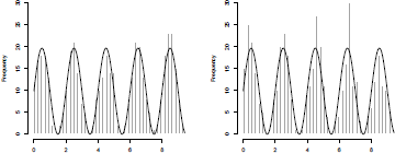
To generate a Poisson process, several algorithms can be considered. In order to illustrate, consider a cyclical Poisson process with intensity
> lambda <- function(t) 100*(sin(t*pi)+1)
so that the cumulated intensity is
> Lambda <- function(t) integrate(f=lambda,lower=0,upper=t)$value
Given that the last claim occurred at time t, let be the conditional distribution function of the waiting time before the next claim. Then
From a computational aspect, we just have to invert this function and use a rejection technique algorithm,
> Tmax <- 3*pi
> set.seed(l)
> t <- 0; X <— numeric(0)
> while(X[length(X)] <= Tmax){
+ Ft <- function(x) 1-exp(-Lambda(t+x)+Lambda(t))
+ x <- uniroot(function(x) Ft(x)-runif(1),interval=c(0,Tmax))$root + t <- t+x + X <- c(X,t)}
> X <- X[-which.max(X)]
To visualize the cycle of occurrences, let us consider the following histogram:
> hist(X,breaks=seq(0,3*pi,by=pi/32),col="grey",
+ border="white",xlab="",main="")
> lines(seq(0,3*pi,by=.02),lambda(seq(0,
+ 3*pi,by=.02))*pi/32,lwd=2)
See Figure 2.16. Pasupathy (2010) suggested also to use a rejection technique as an alternative. What we need is an upper bound for the intensity process. A natural upper bound is a constant one, obtained using max ,
> lambda.up <- 200
The code to generate a Poisson process is
> set.seed(1)
> t <- 0; X <- t
> while(X[length(X)]<=Tmax){
+ u <- runif(1)
+ t <- t-log(u)/lambda.up
+ if(runif(1)<=lambda(t)/lambda.up) X <- c(X,t)}
> X <- X[-c(1,which.max(X))]
The two algorithms can be visualized in Figure 2.16.
Consider a Poisson process with intensity . If we keep each point according to some Bernoulli distribution B(p), then the new point process is also a Poisson process, with intensity . A standard application is obtained when we consider some deductible d. If the occurrence of claims, for some reinsurer is driven by a Poisson process, with intensity. , and if individual losses have distribution F, then the process of claims above the deductible is a Poisson process with intensity This property will be extremely important in compound Poisson processes (introduced in the next section).
2.5.3 From Poisson Processes to Levy Processes
A natural extension to the Poisson process is the compound Poisson process, extremely useful to model a surplus process of an insurance company. Given a Poisson process () and a collection of i.i.d. random variables define
To generate such a process on time interval [0, Tmax], we need to generate a collection of variables, for claims arrival, and claim sizes given a function randX that generates independent variables ’s, such as
> randX <- function(n) rexp(n,1)
The code can be the following:
> rCompPoissonProc <- function(Tmax=1,lambda=rate,rand){
+ N <- rpois(n=1,lambda*Tmax)
+ X <- randX(N)
+ vect.T <- NULL
+ if(N>0) vect.T=sort(runif(N))*lambda*T
+ return(list(T=vect.T,W=diff(c(0,vect.T)),X=X,N=N))}
> set.seed(1)
> rCompPoissonProc(Tmax=5,rand=randX)
$T
[1] 0.3089314 0.8827838 1.0298729 3.4351142
$W
[1] 0.3089314 0.5738524 0.1470891 2.4052414
$X
[1] 1.1816428 0.1457067 0.1397953 0.4360686
$N
[1] 4
Based on such a simulation, it is possible to define a function :
> set.seed(1)
> compois <- rCompPoissonProc(Tmax=5,rand=randX)
> St <- function(t){sum(compois$X[compois$T<=t])}
and we can visualize this trajectory (left part of Figure 2.17) using

Sample path of a compound Poisson process on the left, and a Brownian motion on the right.
> time <- seq(0,5,length=501)
> plot(time,Vectorize(St)(time),type="s")
> abline(v=compois$T,lty=2,col="grey")
To generalize to Lévy processes, we simply have to have a random part, corresponding to a Brownian motion,
The Brownian () motion satisfies, for all n
where increments are i.i.d. Gaussian random variables, centered, with variance T/n. Thus, to generate a trajectory of the Brownian motion on [0, Tmax], we have to discretize, and given n, use the function above,
> n <- 1000
> h <- Tmax/n
> set.seed(1)
> B <- c(0,cumsum(rnorm(n,sd=sqrt(h))))
The analogous function St would be, here,
> Bt <- function(t){B[trunc(n*t/Tmax)+1])}
and we can visualize this trajectory (right part of Figure 2.17) using
> time <- seq(0,5,length=501)
> plot(time,Vectorize(Bt)(time),type="s")
(where level curves related to quantiles of Gaussian random variables were added).
Based on these two functions, it is then possible to generate a trajectory for the Lévy process,
> mu <- lambda*rate
> L <- function(t) -mu*t+St(t)+Bt(t)
but one should keep in mind that if we can generate the first continuous time process (compound Poisson), then we can only generate an approximation of the second one (Brownian motion); first, we have to specify the grid (choosing n), and then, on that grid, we generate a path.
2.5.4 Ruin Models
Ruin theory deals with the study of stochastic processes linked to the wealth of an insurer; see Asmussen & Albrecher (2010) or Dickson (2010) for a recent survey. A reserve risk process is considered. The initial model of Cramer-Lundberg assumes that the surplus of an insurance company at time t is represented by
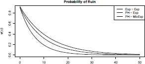
where u is the initial surplus, c is the premium rate, are i.i.d. successive claim amounts and is the claim arrival process assumed to be a Poisson process of intensity (see Rolski et al. (1999) for more details on the Poisson process). Andersen (1957) generalized this model by proposing a renewal process for the claim arrival process (the claim waiting times are denoted by . When claim severities and claim waiting times follow a phase-type distribution, closed-form formulas exist for the ruin probability,
see Asmussen & Rolski (1991). We provide below examples of that article.
> psi <- ruin(claims = "e", par.claims = list(rate = 1/0.6),
+ wait = "e", par.wait = list(rate = 1/0.6616858))
Consider Phase-type claims, exponential inter-arrival times:
> p <- c(0.5614, 0.4386)
> r <- matrix(c(-8.64, 0.101, 1.997, -1.095), 2, 2)
> lambda <- 1/(1.1 * mphtype(1, p, r))
> psi2 <- ruin(claims = "p", par.claims = list(prob = p, rates = r),
+ wait = "e", par.wait = list(rate = lambda))
Consider Phase-type claims, a mixture of two exponentials for inter-arrival times:
> a <- (0.4/5 +0.6) * lambda
> psi3 <- ruin(claims = "p", par.claims = list(prob = p, rates = r),
+ wait = "e", par.wait = list(rate = c(5 * a, a), weights =
+ c(0.4, 0.6)), maxit = 225)
> plot(psi, from =0, to = 50)
> plot(psi2, add=TRUE, lty=2)
> plot(psi3, add=TRUE, lty=3)
> legend("topright", leg=c("Exp - Exp", "PH - Exp",
+ "PH - MixExp"), lty=1:3, col="black")
2.6 Copulas and Multivariate Distributions
This final section deals with distributions of multivariate random vectors . Due to the growing literature (see Frees & Valdez (1998), Embrechts et al. (2001), Frees & Wang (2006), among others) on copulas during the past decade (defined as multivariate distribution functions of random vector with uniform marginals), we focus on copulas in this section.
2.6.1 Definition of Copulas
Let be the distribution function of X with marginals that is,
As has the same distribution as for U a uniform variate, it is easily checked that . A copula function C is a multivariate distribution function such that The C function is bounded by the so-called Fréchet bound as
generally denoted by W(u) and M(u); see Nelsen (2006) for a recent introduction. By the Sklar theorem (from Sklar (1959)) for any random vectors X with marginals , there exists a copula function C such that
for all . Note that the copula C is unique on the support of X, and not otherwise. Let us note that in the independent case, the copula function is simply . As described below, classical multivariate distributions such as the multivariate Gaussian distribution and the multivariate Pareto distribution can be represented using a copula function. Note further that there exists a copula function C* such that
for all . This copula C* will be called survival or dual of C. If U has distribution function C, then 1 — U has distribution function C*.
2.6.2 Archimedean Copulas
A wide class of copulas is given by the family of Archimedean copulas. An Archimedean copula is characterized by a generator function such that
where and is infinitely differentiable, completely monotone and invertible (weaker conditions can be required for specific dimensions d). We refer to Theorem 2.1 of Marshall & Olkin (1988) for the construction of Archimedean copulas. In this family, the three most classical copulas are the Gumbel copula , the Frank copula and the Clayton copula for a parameter .
We get the following copula function:
- Gumbel:
- Frank:
- Clayton: dimesions
The survival Clayton defined as is linked to the multivariate Pareto distribution. According to Arnold (1983), the multivariate Pareto distribution is characterized by the following survival function:
The marginal distribution of is also Pareto distributed, as . It is easy to check that .
2.6.3 Elliptical Copulas
Before introducing elliptic copulas, we define elliptical distributions. A random variable X has an elliptical distribution if its characteristic function satisfies
for some parameters and some function . Generally a random vector X follows an elliptical distribution if its characteristic function verifies
for some vector , some positive definite matrix , and some function . For such a distribution, the density function is given by
some function such that and some normalizing constant . We get the multivariate normal distribution when with mean vector and covariance matrix , the multivariate Student distribution with m degrees of freedom when See Fang et al. (1990) or Genton (2004) for more details on elliptical distributions.
An elliptical copula is defined as
where H is a multivariate distribution with marginals belonging to the elliptical family. In particular for a symmetric positive definite matrix , the Gaussian and the student copulas are defined as
-
Gaussian
where is the quantile function of the standard normal distribution.
-
Student
Where is the quantile of a Student distribution with m > 0 degrees of freedoms.s
2.6.4 Properties and Extreme Copulas
Copulas presented in the previous subsections have a density function because the copula function is differentiable with respect to all variables on the unit hypercube. The dependence induced by a particular copula can be quantified through the theory of concordance measures introduced by Scarsini (1984). The two main measures of concordance are Kendall’s tau and Spearman’s rho. Kendall’s tau for a bivariate vector (X, Y) is defined as
where is an independent replicate of (X, Y). Similarly, Spearman’s rho for (X, Y) is defined as
where and are independent replicates of (X, Y). As these two measures satisfy the criteria of concordance measures, means that the copula of (X, Y) is the upper Frechet bound, and τ(X, Y) = 0 means that the copula of (X, Y) is the independent copula (the same holds for p(X, Y)). In the bivariate case, closed-form formulas are available for the copulas previously presented; see, for example, Nelsen (2006) and Joe (1997).
A desirable feature of copulas lies in the fact that they can model dependence between two or more variables with or without a tail dependency. This is characterized by the tail dependance coefficients. The upper tail coefficient of (X, Y) is defined as
while the lower tail coefficient is obtained considering
When X, Y have a continuous distribution with a dependency given by a copula , those coefficients can be rewritten as
For the copulas presented here, we have except for the Gumbel copula and the Student copula except for the Clayton copula and the Student copula .In other words, copulas with cannot model dependence at the right-hand tail.
Another desirable property of copulas can be the max-stability. A copula function C is max-stable if
for all k > 0. This property is linked to the extreme value theory because the right-hand side is the copula of component-wise maxima of a random vector sample , where the ’s have copula C. Copulas verifying this property are called extreme copulas: The Gumbel and the Hiisler-Reiss copulas belong to this family. The Hiisler-Reiss copula is defined as follows in the bivariate case,
where is the distribution function of the standard normal distribution.
2.6.5 Copula Fitting Methods
There are four main methods to calibrate copulas which differ on how the marginals are considered in the fitting process. Consider a sample of random vectors and corresponding observations
where the ith marginal has a density and a distribution function . A (full) maximum likelihood estimation is the first option, which consists of maximizing the likelihood
α being the parameter of the copula C and being the parameter for the ith marginal distribution. The optimization is carried out over the whole parameter space.
The second estimation method is the method of moments which consists, as in the univariate, of matching theoretical moments and empirical moments. Marginal parameters θ i are set by equalizing the empirical moments of the sample , while the copula parameters a are determined by matching Kendall’s tau or Spearman’s rho.
The third estimation, called inference for margins, is a two-step procedure. First, marginal distributions are fitted by maximum likelihood, and then a pseudo sample is defined as
for i = 1,..., n. Then the copula is fitted on by maximizing the likelihood
The inference for margins method takes advantage of the two steps to reduce the dimension of the likelihood from to α. Finally, the canonical maximum likelihood method is similar to the inference for margins and consists of replacing the parametric estimate by the non-parametric estimates in the pseudo data. That is to say, which further simplifies to . In the following section, we only consider the inference for margins method.
2.6.6 Application and Copula Selection
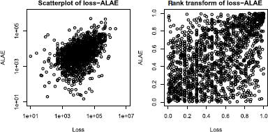
Numerical illustrations of copulas and their estimation are carried out on the loss-ALAE dataset used in Frees & Valdez (1998) and Klugman & Parsa (1999). The dataset consists of 1,500 general liability claims (expressed in USD) where each claim is a two-component vector: an indemnity payment (loss) and an allocated loss adjustment expense (ALAE).
> data(lossalae)
> par(mfrow=c(1,2))
> plot(lossalae, log="xy", main="Scatterplot of loss-ALAE")
> plot(apply(lossalae, 2, rank)/NROW(lossalae),
+ main="rank transform of loss-ALAE")
In Figure 2.19, we plot the scatterplots of the data (xi,yi) and the empirical distributions evaluated at (xj,yj), that is,
On this dataset, we choose to fit the following bivariate copulas:
- (i) Gaussian copula CGa(.,.; p),
- (ii) Student copula CSt(.,.; p, m),
- (iii) Gumbel copula CGu(.,.; α),
- (iv) Frank copula CF(.,.; α)
- (v) Hiisler-Reiss copula CHR(.,.; a).
We use the implementation done in the fCopulae package (part of the Rmetrics project, see https://www.rmetrics.org/; see also Chapter 11 and chapter 13). For convenience, we define the following functions
> dnormcop <- function(U, param)
+ as.numeric(dellipticalCopula(U, rho=param[1], type="norm"))
> dtcop <- function(U, param)
+ as.numeric(dellipticalCopula(U, rho=param[1], type="t",
+ param=param[2]))
> dgumcop <- function(U, param)
+ as.numeric(devCopula(U, type="gumbel", param=param[1]))
> dHRcop <- function(U, param)
+ as.numeric(devCopula(U, type="husler.reiss", param=param[1]))
> dfrankcop <- function(U, param)
+ as.numeric(darchmCopula(U, type="5", alpha=param[1]))
In addition to finding an appropriate copula, a choice of distribution must be done for marginals. A Pareto chart on both marginals shows that they follow heavy-tailed distributions.
> paretochart <- function(x, ...)
+ plot(-log((1:length(x))/(length(x)+1)), log(sort(x)), ...)
> paretochart(lossalae$Loss)
> paretochart(lossalae$ALAE)
Therefore, we choose a Pareto type II distribution and a lognormal distribution for candidate distributions of marginals. As there is no package fitting copulas for any kind of copula, we implement the inference for margins method in the following function:
> fit.cop.IFM.2 <- function(obs, copula, marg, arg.margin=list(),
+ method.margin="mle", arg.cop=list(), initpar, ...)
+ {
+ Obs1 <- obs[,1]
+ Obs2 <- obs[,2]
+ if(marg %in% c("exp","gamma","lnorm","pareto","burr")){
+ Obs1 <- Obs1[Obs1 > 0]
+ Obs2 <- Obs2[Obs2 > 0]}
+ marg1 <- do.call(fitdist, c(list(data= Obs1, distr=marg,
+ method=method.margin), arg.margin))
+ marg2 <- do.call(fitdist, c(list(data= Obs2, distr=marg,
+ method=method.margin), arg.margin))
+ comput.cdf <- function(fit, obs) {
+ para <- c(as.list(fit$estimate), as.list(fit$fix.arg))
+ distname <- fit$distname
+ pdistname <- paste("p", distname, sep = "")
+ do.call(pdistname, c(list(q = obs), as.list(para)))}
+ pseudomarg1 <- comput.cdf(marg1, Obs1)
+ pseudomarg2 <- comput.cdf(marg2, Obs2)
+ U <- cbind(pseudomarg1, pseudomarg2)
+ copLogL <- function(x) {
+ if(arg.cop$lower <= x && arg.cop$upper >= x) + res <- -sum(remove.naninf(log(copula(U, param=x))))
+ else res <- Inf + return(res)}
+ resopt <- optim(par=initpar, fn=copLogL, method="L-BFGS-B",
+ lower=arg.cop$lower, upper=arg.cop$upper, ...)
+ list(marg1=marg1, marg2=marg2, copula=
+ list(id="arg.cop$name, alpha=resopt$par))}
> remove.naninf <- function(x)
+ x[!is.nan(x) & is.finite(x)]
The copulas are now fitted using the function fit.cop.IFM.2 by defining the corresponding arg.cop argument. Note that the marginal distributions are fitted using fitdist.
> library(fCopulae)
> argnorm <- list(length=1, lower=0, upper=1, id=""Gaussian")
> argt <- list(length=2, lower=c(0,0), upper=c(1,1000),
+ id=""Student")
> arggum <- list(length=1, lower=1, upper=100, id=""Gumbel")
> argHR <- list(length=1, lower=0, upper=1000, id=""Husler-Reiss")
> argfrank <- list(length=1, lower=-1000, upper=1000, id=""Frank")
> fgausspareto <- fit.cop.IFM.2(lossalae, copula= dnormcop,
+ marg="pareto", arg.margin=list(start=list(shape=10, scale=100),
+ lower=c(1, 1/2)), arg.cop= argnorm, initpar=1/2)
> ftpareto <- fit.cop.IFM.2(lossalae, copula= dtcop,
+ marg="pareto", arg.margin=list(start=list(shape=10, scale=100),
+ lower=c(1, 1/2)), arg.cop= argt, initpar=c(1/2, 4))
> fgumbelpareto <- fit.cop.IFM.2(lossalae, copula= dgumcop,
+ marg="pareto", arg.margin=list(start=list(shape=10, scale=100),
+ lower=c(1, 1/2)), arg.cop= arggum, initpar=10)
> fHRpareto <- fit.cop.IFM.2(lossalae, copula= dHRcop,
+ marg="pareto", arg.margin=list(start=list(shape=10, scale=100),
+ lower=c(1, 1/2)), arg.cop= argHR, initpar=10)
> ffrankpareto <- fit.cop.IFM.2(lossalae, copula= dfrankcop,
+ marg="pareto", arg.margin=list(start=list(shape=10, scale=100),
+ lower=c(1, 1/2)), arg.cop= argfrank, initpar=10)
> recap <- function(x){
+ res <- c(alpha=x$copula$alpha, x$marg1$estimate, x$marg2$estimate) + if(length(res) < 6)
+ res <- c(res[1], NA, res[2:5])
+ res <- as.matrix(res)
+ colnames(res) <- x$copula$name
+ res}
> round(cbind(recap(fgausspareto), recap(ftpareto), + recap(fHRpareto), recap(fgumbelpareto),
+ recap(ffrankpareto) ), 4)
Gaussian Student Husler-Reiss Gumbel Frank
alpha 0.4783 0.4816 1.1133 1.4444 3.1140
NA 9.6475 NA NA NA
shape 1.2377 1.2377 1.2377 1.2377 1.2377
scale 16228.2572 16228.2572 16228.257 16228.2572 16228.2572
shape 2.2230 2.2230 2.2230 2.2230 2.2230
scale 15133.3463 15133.3463 15133.3463 15133.3463 15133.3463
The level of dependency seems low as the value of the first parameter is either close to 1 (for non-elliptic copulas) or close to 0 for elliptic copulas. Unsurprisingly, the fitted parameters of the marginal distributions are identical. In order to assess the quality of the fit, we look at the tail coefficients and which are computable given a copula. They can be estimated on data by using a non-parametric estimate of C(t,t), that is, the empirical bivariate distribution function This is done by the following function:
> Lemp <- function(u, obs)
+ sapply(1:length(u), function(i)
+ 1/NROW(obs)*sum(obs[,1] <= u[i] & obs[,2] <= u[i]))/u
> Uemp <- function(u, obs)
+ (1-2*u+sapply(1:length(u), function(i)
+ 1/NROW(obs)*sum(obs[,1] <= u[i] & obs[,2] <= u[i])))/(1-u)
> Lcop <- function(u, pcop, param=param)
+ pcop(cbind(u, u), param=param)/u
> Ucop <- function(u, pcop, param=param)
+ (1-2*u+pcop(cbind(u, u), param=param))/(1-u)
The plot of the two tail coefficients is now possible.
> u <- seq(0, 0.4, length=101)
> rklossalae <- apply(lossalae, 2, rank)/NROW(lossalae)
> plot(u, Lemp(u, rklossalae), type="l", main="Lower coefficient",
+ ylim=c(0,.6), xlab="u", ylab="L(u)")
> lines(u, Lcop(u, pgumcop, fgumbelpareto$copula$alpha), lty=2)
> lines(u, Lcop(u, pHRcop, fHRpareto$copula$alpha), lty=3)
> lines(u, Lcop(u, ptcop, ftpareto$copula$alpha), lty=4, col="grey25")
> lines(u, Lcop(u, pnormcop, fgausspareto$copula$alpha), lty=5, col="grey25")
> lines(u, Lcop(u, pfrankcop, ffrankpareto$copula$alpha), lty=6, col="grey25")
> legend("bottomright", lty=1:6, col=c(rep("black", 3), rep("grey25", 3)),
+ leg=c("emp.", "Gumbel","Husler-Reiss","Student","Gaussian","Frank"))
As shown on Figure 2.20, the tail coefficients are best approximated by the extreme copulas: Gumbel and Husler-Reiss. When considering Kendall’s tau or Spearman’s rho, these two copulas are also reasonably good. Kendall’s tau is here:

> cbind(emp=cor(lossalae, method="kendall")[1,2],
+ Frank=taufrankcop(ffrankpareto$copula$alpha),
+ Gumbel= taugumcop(fgumbelpareto$copula$alpha),
+ HR= tauHRcop(fHRpareto$copula$alpha),
+ Gauss = taunormcop(fgausspareto$copula$alpha),
+ Student = tautcop(ftpareto$copula$alpha))
emp Frank Gumbel HR Gauss Student
Tau 0.3154175 0.3171107 0.3076705 0.3008525 0.3174771 0.3198691
while Spearman’s rho is
> cbind(emp=cor(lossalae, method="spearman")[1,2],
+ Frank=rhofrankcop(ffrankpareto$copula$alpha),
+ Gumbel= rhogumcop(fgumbelpareto$copula$alpha),
+ HR= rhoHRcop(fHRpareto$copula$alpha),
+ Gauss = rhonormcop(fgausspareto$copula$alpha),
+ Student = rhotcop(ftpareto$copula$alpha))
emp Frank Gumbel HR Gauss Student
Rho 0.451872 0.4622724 0.4424486 0.4360027 0.4500000 0.4500000
Therefore, we continue the analysis only with the Gumbel and Husler-Reiss copulas.
Given a copula, quantities of interest can be estimated by a Monte-Carlo method. Focusing on the distribution of the total expense, that is, the sum of loss and ALAE, we simulate this sum with the following template function:
> simul.cop.2 <- function(n, rcopula, fit){
+ U <- rcopula(n, fit$copula$alpha)
+ qmarg1 <- paste("q", fit$marg1$distname, sep="")
+ qmarg2 <- paste("q", fit$marg2$distname, sep="")
+ cbind(
+ X1=do.call(qmarg1, c(list(p=U[,1]), fit$marg1$estimate)),
+ X2=do.call(qmarg2, c(list(p=U[,2]), fit$marg2$estimate))
+)}
where rcopula() is the copula random generator defined as
> rgumcop <- function(n, param)
+ revCopula(n, type="gumbel", param=param[1])
> rHRcop <- function(n, param)
+ revCopula(n, type="husler.reiss", param=param[1])
> rindep <- function(n,param)
+ cbind(runif(n), runif(n))
Choosing a sample size of n = 1e4, we plot the empirical distribution functions of the sum for the Gumbel, the Husler-Reiss and the independent copulas.
> sumlossalae <- rowSums(lossalae)
> n <- 10"4
> sumgumpareto <- rowSums(simul.cop.2(n, rgumcop, fgumbelpareto))
> sumHRpareto <- rowSums(simul.cop.2(n, rHRcop, fHRpareto))
> sumindeppareto <- rowSums(simul.cop.2(n, rindep, fgumbelpareto))
> plot(ecdf(sumlossalae), log="x", main="", xlim=range(sumlossalae))
> z <- 10"seq(1, log(max(sumlossalae)), length=201)
> lines(z, ecdf(sumgumpareto)(z), lty=2)
> lines(z, ecdf(sumHRpareto)(z), lty=3)
> lines(z, ecdf(sumindeppareto)(z), lty=4)
> legend("bottomright", lty=1:4, col="black",
+ leg=c("emp.", "Gumbel", "Husler-Reiss", "indep."))
On Figure 2.21, we observe that both extreme copulas are particularly adapted for the lossalae dataset, irrespective of the choice of the marginal distribution. Yet, we notice that the choice of the lognormal distribution better suits the tail of the empirical distribution. However, as extreme claims above 1 million dollars are less observed (by definition) than large claims (between 100 thousand and 1 million), the experimenter must take a prudential view of the right-hand tail without overfitting data. The independent copula seems to be a reasonable approximation of the tail of the distribution (yet not of the rest of the distribution).
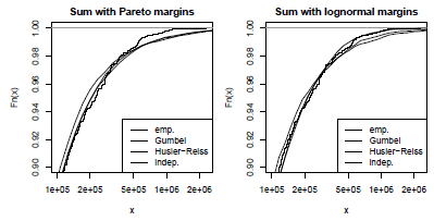
2.7 Exercises
- For these exercises, consider the following vectors,
> set.seed(123)> X1 <- trunc(rlnorm(n=753,5))> X2 <- rgamma(n=267,1.2,.25) fitdistr(X2,"lognormal") - 2.1. Benford’s law is defined on {1, 2,..., 8, 9} as follows:
- Write functions dBenford, pBenford and rBenford that return the density, the (cumulative) distribution function and generate random values according to this distribution.
- 2.2. Given a vector of integers, x, write a function that counts frequency of first digits of elements of x. Write a function, based on Person’s statistics, that tests if Benford’s distribution is relevant, or not (using functions of Exercise 1.). Try this function on X1 .
- Hint: Use function chisq.test to run the test.
- 2.3. Using fitdistr from library MASS, find maximum likelihood estimators if we fit a lognornal distribution to X2.
- 2.4. According to the Kolmogorov-Smirnov test, can we model X2 using a LN(1,1) distribution?
- 2.5. Assume that . Compute . Find (numerically) max
- 2.6. Use function barplot to visualize the probability function associated to Sibuya’s distribution, defined on N by
- 2.7. Without using a loop, write a function rmix(n,p,rf1,rf2,...) that generates n random variables, i.i.d., with distribution the mixture of f1, ..., fn, where p is a vector of probabilities of length n.
- 2.8. Compute the 95% quantile of a compound sum, when N has a negative binomial distribution, with mean 2 and variance 3, and when have a gamma distribution, with mean 100 and variance 150, using the Panjer algorithm.
- 2.9. Compute the 95% quantile of a compound sum, when N has a negative binomial distribution, with mean 2 and variance 3, and when have a gamma distribution, with mean 100 and variance 150, using Monte Carlo simulations.
- 2.10. Fit a gamma and a lognormal distribution to data(danishuni) from library CASdatasets. Which model gives the highest 95% quantile. Compare it with the empirical one.
- 2.11. Fit a gamma and a lognormal distribution to lossalae$ALAE from library CASdatasets. Which model gives the highest 95% quantile. Compare it with the empirical one.
- 2.12. Using a gamma distribution on lossalae$ALAE, what would be the expected value, given that lossalae$ALAE is larger than 10,000.
- 2.13. From results mentioned in Section 2.1.3 and functions associated to phtype, write functions dErlang(x,k,lambda), pErlang(x,k,lambda) and rErlang(n,k,lambda).
- 2.14. Fit a copula on the following sample:
> n <- 1500> set.seed(123)> theta <- rgamma(n,.5)> U <- cbind(rank(rexp(1500,rate=theta))/(n+1),+ rank(rexp(1500,rate=theta))/(n+1)) - 2.15. Given a > 0, fit a truncated distribution to the following sample:
> n <- 1500> a <- 1> set.seed(123)> X <- rep(NA,n)> for(i in 1:n){> x <- a; v<- 2+ while(v*x>a) v<- runif(1); x<-sqrt(a"2-2*log(runif(1)))+ X[i] <- x +} - 2.16. Fit a distribution to the following sample:
> n <- 1500> set.seed(123)> f <- function(v) -v[1]*log(v[2]*v[3])> X <- apply(matrix(runif(3*n),n,3),1,f) - 2.17. Fit a distribution to the following sample:
> n <- 1500> set.seed(123)> f <- function(v) log((v[1]*v[2])/(v[3]*v[4]))> X <- apply(matrix(runif(4*n),n,4),1,f)Hint: It is the density of the sum of two independent and identically distributed random variables.
- 2.18. Fit a distribution to the following sample:
> n <- 1500> set.seed(123)> a <- .4; b <- .2> U <- runif(n)~(1/a)> V <- runif(n)~(1/b)> X <- (U/(U+V))[U+V <= 1] - 2.19. Fit a distribution to the following sample:
> n <- 1500> set.seed(123)> a <- 17; b <- 12> B <- rbeta(n,a,b)> X <- b*B/(a*(1-B)) - 2.20. Fit a distribution to the following sample:
> n <- 1500> set.seed(123)> B <- rbeta(n,a/2,a/2)> X <- sqrt(a)*(B-.5)/sqrt(B*(1-B)) - 2.21. Consider the following counting process, with sequence of arrival times T:
> Tmax <- 20> set.seed(123)> T <- 0> while(max(T)<=Tmax) T<-c(T,sqrt(max(T)"2+2*rexp(1))) - Assuming that this sequence is generated from a non-homogeneous Poisson process, suggest values for an affine intensity .