
Chapter 13
Portfolio Allocation
Yohan Chalabi
ETH Zuürich
Zürich,Switzerland
Diethelm Wiirtz
ETH Zurich Zurich,
Switzerland
13.1 Introduction
Nobel Laureate Harry H. Markowitz provided one of the first formulations of portfolio allocation as an optimization problem (Markowitz (1952)); since then, portfolio allocation has been widely studied and numerous models have been introduced, although the underlying concepts have remained the same. As summarized by Meucci (2009), portfolio allocation can be viewed as a method of maximizing the degree of satisfaction of the investor. For example, one investor might seek a portfolio that minimizes risk represented by a covariance estimator of the daily returns on assets, whereas another might consider risk in terms of the draw-down of wealth over a given time period.
This chapter takes a step-by-step approach to portfolio allocation by introducing the reader to portfolio optimization using R, thus allowing the reader to implement his or her own routines in the process. We deliberately do not use third-party packages so that users can more readily grasp the principles behind portfolio optimization using R. The examples are chosen to be sufficiently brief to be represented by a few lines of code, although general enough to be extended to more complex situations. We take care to introduce problems that require different types of solvers, so that the reader can extend the code snippets to meet their own needs. The packages used in this chapter are Rglpk, quadprog, Rsolnp, DEoptiom, and robustbase, which can be installed as follows:
> library(Rglpk)
> library(quadprog)
> library(Rsolnp)
> library(DEoptim)
> library(robustbase)
Before describing the details of R implementation, we first review in Section 13.2 the portfolio optimization problems that we will be using in this chapter. In Section 13.3, we introduce the dataset that is used in the R code snippets. Section 13.5 introduces typical portfolio problems, and Section 13.6 introduces two graphical approaches for comparing sets of feasible portfolios, which include the efficient frontier and the weighted return plot. Section 13.7 concludes the chapter and includes recommendations for third-party R packages that can be used to extend the portfolio problems presented in this chapter.
13.2 Optimization Problems in R
13.2.1 Introduction
We first review the method for solving optimization problems using R. The optimization field is wide, and optimization problems can be classified on the basis of whether or not a dedicated algorithm exists to solve the problem, and if so, on the type of algorithm that is used in the solution. In this section, we review the optimization problems required for solving the examples in this chapter.
Several algorithms and packages are available for solving a given optimization problem. For simplicity, in this chapter we consider one optimization solver for each type of optimization problem considered. Our selection criteria are that the package is readily available in R, it can model the constraint used in the examples, it is open source, and it is actively maintained. However, readers should bear in mind that many solver routines are available, and the selection of a routine for a given optimization problem should be carefully investigated. Types of solvers in R include (1) optimization routines that are available by default in the base environment. The general-purpose nonlinear optimization routines in R are optim() and nlminb(); however, these routines only support simple bound constraints and do not provide sufficient solvers for our portfolio examples. (2) Several third-party packages are available for implementation of different optimization algorithms. The packages may be available either in the R environment or in external libraries (the libraries may not be shipped with the R package for licensing reasons, or because they require external installation). (3) Optimization solvers in R may interface with a dedicated optimization platform; such platforms typically have their own modeling languages, such as the AMPL modeling language. Although an interface to an external platform does not provide a pure R approach, it offers access to a large set of both open-source and commercial solvers. Indeed, the main drawback of using an optimization routine is that each routine expresses the programming problem in terms of different input arguments, which requires the user to first understand how each interface functions.
The remainder of this section reviews linear, quadratic, and nonlinear optimization problems. The optimization R packages are presented, and wrapper functions are implemented so that each function has a common interface, thus easing implementation of the ensuing portfolio optimization problems.
13.2.2 Linear Programming
For x∈ℝn , a set of vector variables subject to linear equality and inequality constraints, the linear programming problem (LP) can be formulated as
minimizexcTxsubject toAeqx=aeq,(13.1)Ax≥a
where Aeq and a eq are the matrix and vector coefficients, respectively, describing the equality linear constraints; A and a are the matrix and vector coefficients, respectively, describing the inequality linear constraints; and c is the vector of coefficients of the objective function.
At the time of writing , the R packages that provide linear programming solvers are, as reported in the Optimization and Mathematical Programming CRAN Task View Theussl (2013): boot, clpAPI, cplexAPI, glpkAPI, limSolve, linprog, lpSolve, lpSolveAPI, quantreg, rcdd, Rcplex, Rglpk, Rmosek, and Rsymphony. In this chapter, we use the Rglpk package; Rglpk, which was developed and is maintained by Kurt Hornik and Stefan Theussl (Hornik & Theussl (2012)), is a high-level interface of the GNU Linear Programming Kit (GLPK), which solves linear as well as mixed-integer linear programming (MILP) problems.
The arguments for the R function in the GLPK routine, Rglpk_solve_LP(), are
> args(Rglpk_solve_LP)
function (obj, mat, dir, rhs, bounds = NULL, types = NULL, max = FALSE, control = list(), ...)
NULL
where obj is the vector holding the linear coefficients of the objective function, mat is the general constraint matrix, dir describes the direction and types of inequalities, and rhs is the right-hand side vector of the constraints. The remaining arguments are not required for our application.
Following the formulation of the linear programming problem in Equation 13.1, our wrapper function becomes
> LP_solver <- function(c, cstr = list(), trace = FALSE) {
+
+ Aeq <- Reduce(rbind, cstr[names(cstr) %in% "Aeq"])
+ aeq <- Reduce(c, cstr[names(cstr) %in% "aeq"])
+ A <- Reduce(rbind, cstr[names(cstr) %in% "A"])
+ a <- Reduce(c, cstr[names(cstr) %in% "a"])
+
+ sol <- Rglpk_solve_LP(obj = c,
+ mat = rbind(Aeq, A),
+ dir = c(rep("==", nrow(Aeq)),
+ rep(">=", nrow(A))),
+ rhs = c(aeq, a),
+ verbose = trace)
+
+ status <- sol$status
+ solution <- if (status) rep(NA, length(c)) else sol$solution
+ list(solution = solution, status = status)
+}
Here, the constraints are provided as a list object, where the components of the linear constraints are provided as the named entries, Aeq, A, aeq, and a. Note that the list can have several entries with the same name, a feature that is useful when implementing the portfolio constraints. The Reduce function merges all the entries of the cstr list that have the same name. After the constraints have been constructed, the optimization routine is called. The returned object of LP_solver() is a list with two elements: the first is the optimized solution, and the second is the status of the optimization routine if it has completed successfully. We use the same calling convention for the other optimization routines in this chapter.
13.2.3 Quadratic Programming
Compared to linear programming problems, quadratic programs (QP) contain a quadratic term (xTQx) in the objective function. The linear constraints Aeq, A, aeq , and a remain similar. The quadratic formulation is presented in a canonical form as
minimizexcTx +xTQxsubject toAeqx=aeq,(13.2)Ax≥a,
The R packages providing quadratic solvers are cplexAPI, kernlab, limSolve, LowRankQP, quadprog, Rcplex, and Rmosek. The package selected for use in this chapter is quadprog port (2013). The solve.QP() function implements the dual method of Goldfarb & Idnani (1982, 1983) for solving quadratic programming problems of the form minx−cTx+1/2xTQx with the constraints Ax≥a , where the arguments of solve.QP
> args(solve.QP)
function (Dmat, dvec, Amat, bvec, meq = 0, factorized = FALSE)
NULL
Dmat is the quadratic matrix Q, dvec is the linear part of c in the objective function, Amat defines the constraints matrix A, and bvec is the vector holding the values of a. The argument meq is used to specify how many of the first linear constraints should be considered equality constraints.
The canonical form used in the quadprog package is slightly different from that used in the linear approach. Therefore, a small wrapper is used to maintain a similar canonical form:
> QP_solver <- function(c, Q, cstr = list(), trace = FALSE) {
+
+ Aeq <- Reduce(rbind, cstr[names(cstr) %in% "Aeq"])
+ aeq <- Reduce(c, cstr[names(cstr) %in% "aeq"])
+ A <- Reduce(rbind, cstr[names(cstr) %in% "A"])
+ a <- Reduce(c, cstr[names(cstr) %in% "a"])
+
+ sol <- try(solve.QP(Dmat = Q,
+ dvec = -2 * c,
+ Amat = t(rbind(Aeq, A)),
+ bvec = c(aeq, a),
+ meq = nrow(Aeq)),
+ silent = TRUE)
+ if (trace) cat(sol)
+ if (inherits(sol, "try-error"))
+ list(solution = rep(NA,length(c)), status = 1)
+ else
+ list(solution = sol$solution, status = 0)
+}
Note that the objective function defined in the previous snippet is equal to the canonical form in Equation (13.2) times a factor of 2. However, the solution remains the same as in the canonical formulation as the minimum of both objective functions is attained using the same set of parameter values.
13.2.4 Nonlinear Programming
The canonical form of the nonlinear programming (NLP) model is characterized by a nonlinear objective function, represented by the function f, which has as its argument the vectors of unknown variables x:
minimizexf(x)subject toAeqx=aeq,Ax≥a,(13.3)heqi(x)=0,hi(x)≥0.
The model contains both the linear (Aeq,aeq) and (A,a) , and nonlinear constraints hieq and hi , which are the equality and inequality constraints, respectively. At the time of writing, two R packages are available that can solve NLP problems: Rdonlp2 and Rsolnp. In this chapter, we have selected the open-source package Rsolnp, developed by Ghalanos Ghalanos & Theussl (2012); Rsolnp is based on the SOLNP routine of Ye (1987). SOLNP implements the augmented Lagrange multiplier method with a sequential quadratic programming interior algorithm.
As before, we implement a small wrapper function to maintain a common interface:
> NLP_solver <- function(par, f, cstr = list(), trace = FALSE) {
+
+ Aeq <- Reduce(rbind, cstr[names(cstr) %in% "Aeq"])
+ aeq <- Reduce(c, cstr[names(cstr) %in% "aeq"])
+ A <- Reduce(rbind, cstr[names(cstr) %in% "A"])
+ a <- Reduce(c, cstr[names(cstr) %in% "a"])
+ heq <- Reduce(c, cstr[names(cstr) %in% "heq"])
+ h <- Reduce(c, cstr[names(cstr) %in% "h"])
+
+ leqfun <- c(function(par) c(Aeq par), heq)
+ eqfun <- function(par)
+ unlist(lapply(leqfun, do.call, args = list(par)))
+ eqB <- c(aeq, rep(0, length(heq)))
+
+ lineqfun <- c(function(par) c(A par), h)
+ ineqfun <- function(par)
+ unlist(lapply(lineqfun, do.call, args = list(par)))
+ ineqLB <- c(a, rep(0, length(h)))
+ ineqUB <- rep(Inf, length(ineqLB))
+
+ sol <- solnp(par = par,
+ fun = f,
+ eqfun = eqfun,
+ eqB = eqB,
+ ineqfun = ineqfun,
+ ineqLB = ineqLB,
+ ineqUB = ineqUB,
+ control = list(trace = trace))
+
+ status <- sol$convergence
+ solution <- if (status) rep(NA, length(par)) else sol$pars
+ list(solution = solution, status = status)
+}
Note that implementation of the canonical form used in Equation (13.3) requires more work than is required in the previous cases, as the constraints in solnp() must be directly expressed in terms of functions. Therefore, the linear constraints A and a must be converted to function constraints.
13.3 Data Sources
The first dataset used in this chapter is the EuStockMarkets dataset, obtained from the datasets package that is part of the standard R installation. EuStockMarkets consists of the daily closing prices of major European stock indices from 1991 to 1998, including the German DAX (Ibis), Swiss SMI, French CAC, and UK FTSE. The dataset is readily available and convenient to use, as there is no need to download the data from an external source. The first lines of the dataset are shown in the following code snippet:
> head(EuStockMarkets)
DAX SMI CAC FTSE
[1,] 1628.75 1678.1 1772.8 2443.6
[2,] 1613.63 1688.5 1750.5 2460.2
[3,] 1606.51 1678.6 1718.0 2448.2
[4,] 1621.04 1684.1 1708.1 2470.4
[5,] 1618.16 1686.6 1723.1 2484.7
[6,] 1610.61 1671.6 1714.3 2466.8
Symbols of the NASDAQ indices and U.S. Treasury yields composing the dataset.
IXBK |
NASDAQ Bank |
NBI |
NASDAQ Biotechnology |
IXK |
NASDAQ Computer |
IXF |
NASDAQ Financial 100 |
IXID |
NASDAQ Industrial |
IXIS |
NASDAQ Insurance |
IXUT |
NASDAQ Telecommunications |
IXTR |
NASDAQ Transportation |
FVX |
U.S. Treasury yield 5 years |
TYX |
U.S. Treasury yield 30 years |
Although the EuStockMarkets dataset is sufficient for the presentation of portfolio optimization problems in this chapter, we also would like to show how a larger dataset can be downloaded from a website, converted to an R object, and saved as a binary file for later use, as such examples are closer to real applications of portfolio optimization in R. Thus, the second dataset used in this chapter represents NASDAQ indices and U.S. treasury yields listed in Table 13.3 and in the following code snippet:
> id <- c("IXBK", "NBI", "IXK", "IXF", "IXID", "IXIS", "IXUT",
+ "IXTR", "FVX", "TYX")
The NASDAQ/Treasury historical dataset can be downloaded from the Yahoo! Finance website. At the time of writing, the data can be downloaded in a comma-separated value (csv) format, either manually for each financial index or using a small R function to perform the operations, from http://ichart.finance.yahoo.com/table.csv?s=XYZ, where “XYZ” represents a specific query (note that the URL may change at any time). The R function read.csv() reads the csv file and creates an R object; read.csv is a wrapper function within the general read.table() function, with the arguments set for csv files (see also Chapter 1):
> args(read.csv)
function (file, header = TRUE, sep = ",", quote = """, dec = ".", fill = TRUE, comment.char = "", ...)
NULL
In the next code snippet, we are using the three dots argument to pass further arguments to the underlying read.table() function. The colClasses argument specifies which object class R should transform in each column of the dataset. The first column is converted to a Date class, whereas the other six columns are converted to numerical vectors, according to
> downloadSymbol <- function(symbol) {
+ address <- "http://ichart.finance.yahoo.com/table.csv"
+ url <- paste(address, symbol, sep = "?s=~")
+ read.csv(url, colClasses = c("Date", rep("numeric", 6)))
+}
As an example of the data input procedure, we show the first part of the IXBK index dataset. The dataset is organized in columns; the date is in the first column, followed by open, high, low, and closing prices, followed by the volume and the adjusted closing price,
> head(downloadSymbol("IXBK"))
Date Open High Low Close Volume Adj.Close
1 2013-05-31 2162.60 2167.93 2144.64 2146.29 0 2146.29
2 2013-05-30 2154.76 2174.71 2154.60 2172.63 0 2172.63
3 2013-05-29 2154.69 2163.77 2150.68 2154.01 0 2154.01
4 2013-05-28 2167.72 2183.75 2158.48 2168.55 0 2168.55
5 2013-05-24 2127.13 2145.25 2122.67 2144.84 0 2144.84
6 2013-05-23 2119.05 2134.75 2118.47 2134.68 0 2134.68
To avoid downloading the data at every session, we aggregate the adjusted closing price of the time series into a data.frame and save it as a binary R object. The following code snippet downloads datasets for each symbol using the lapply() function, which returns a list with a data.frame for each symbol. We then use the Reduce() function to successively merge the elements of the list. Using the merge() function, which is similar to the database “join” operation, the data are merged according to their date stamps:
> lprices <- lapply(id, function(symbol) {
+ df <- downloadSymbol(symbol)[,c("Date", "Adj.Close")]
+ names(df) <- c("Date", symbol)
+ df
+})
> prices <- Reduce(function(x, y)
+ merge(x,y, all = TRUE, by = "Date"),
+ lprices)
In the downloaded dataset, missing values are represented by NAs in the merge operation. In the examples in this chapter, data were selected for the period 2003-2006, which is easily accomplished as the first column of the dataset contains the Date argument. Note how we reset the row names of the data.frame object in the next code snippet.
> pos <- (prices$Date >= as.Date("2003-01-01") &
+ prices$Date < as.Date("2007-01-01"))
> prices <- prices[pos,]
> isNA <- rowSums(sapply(prices[-1], function(x) is.na(x)))
> isNA <- as.logical(isNA)
> prices <- prices[!isNA,]
> rownames(prices) <- NULL
The obtained data.frame is saved as an R object in an “rds” binary file format, according
to
> saveRDS(prices, file = "data.rds")
Binary files created using R have the advantage that their format is independent of the operating system. Thus, datasets can be saved and loaded in different operating systems that support R. Moreover, by default, the binary file is compressed for optimized storage, which can become important when dealing with large datasets. R binary files can be loaded using the readRDS() function as follows:
prices <- readRDS("data.rds")
Note, however, that the working directory of the R session must either be the same as the directory in which the dataset is saved, or the appropriate path to the saved file must be recalled.
13.4 Portfolio Returns and Cumulative Performance
Using the downloaded dataset, we converted price data into values that can be modeled by a statistical distribution. The most common transformation yields arithmetic returns, defined at time t by
rt=Pt−Pt−1Pt−1=PtPt−1−1 ,
where is Pt the price of the financial instrument at time t. Based on the returns at time t, the aggregation of daily returns over period T is
rt=PTP0−1=PTPT−1PT−1PT−2...P1P0−1=∏Tt=1PtPt−1
Given a portfolio wealth at time t(Wt) , which corresponds to the sum of the values of
its components, Wt=∑iPi,t , the portfolio return at time t(Rt) becomes
Rt=1Wt−1(Wt−Wt−1)=1Wt−1(P1,t+P2,t+....+PN,t−1−P2,t−1−...−PN,t−1)=1Wt−1[(P1,t−P1,t−1)+(P2,t−P2,t−1)+...+(PN,t−PN,t−1)]=1Wt−1(P1,t−1r1+P2,t−1r2+...+P2,t−1r2)
The portfolio return is therefore the sum of its component returns weighted by their allocation
Rt=∑NiPt−1Wt−1ri=∑Niwiri
These data allow calculation of the daily arithmetic returns for the dataset presented in the previous section, according to
> x <- sapply(prices[-1],
+ function(x) x[-1] / x[-length(x)] - 1)
Note that the sapply() function is used to apply an operation to each column of the object prices that is of class data.frame.
If, for some reason, the indices cannot be downloaded, the EuStockMarkets dataset can be used as an alternative data source:
> # x <- apply(EuStockMarkets, 2,
> # function(x) x[-1] / x[-length(x)] - 1)
Given the asset returns r and the portfolio weights w, the cumulative performance at time t can be calculated as
Wt=W0∏ti(1+xtTw)
where W0 is the initial portfolio wealth. The cumulative portfolio performance can then be implemented as follows, where the default initial portfolio wealth is set at $1000:
> pftPerf <- function(x, w, W0 = 1000) {
+ W0 * cumprod(c(1, 1 + x %*% w))
+}
The method is illustrated by the following code snippet, which plots (Figure 13.1) the cumulative performance for the equally weighted portfolio.
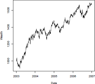
Cumulated performance of the equally weighted portfolio with an initial wealth of $1000.
> nc <- ncol(x)
> w <- rep(1/nc, nc)
> plot(prices$Date, pftPerf(x, w), type = "l",
+ main = "Portfolio Cumulated Performance",
+ xlab = "Date", ylab = "Wealth")
13.5 Portfolio Optimization in R
13.5.1 Introduction
In this chapter, we adopt the general formulation for portfolio optimization, which consists of minimization of a risk measure given a target reward and operational constraints. We first present the mean-variance portfolio for which the risk measure is represented by the covariance matrix of the portfolio. In the second example, the risk is measured as a conditional Value-at-Risk. The third example considers the minimization of drawdowns. In addition to risk measures, an important aspect of portfolio optimization is the formulation of constraints that reflect either operational or decisional constraints. Before presenting the portfolio models, we first review different types of constraints that are implemented in the form of an R function, and which correspond to the canonical optimization problems presented in Section 13.2.
Target Reward
The first constraint is set by the goal to achieve the target reward measure. The target reward constraint ˉr is given by the weights w and average returns μ of each of the components, according to μTw=ˉr . The constraint is given in terms of the matrix and vector coefficients Aeq and aeq , respectively, according to
> targetReturn <- function(x, target) {
+ list(Aeq = rbind(colMeans(x)), aeq = target)
+}
Full Investment
The full investment constraint states that all capital must be invested in the portfolio. The full investment constraint corresponds to the condition in which the sum of all weights w is equal to 100%, where the weights correspond to portions of the capital allocated to a given component. We obtain the R function for the full investment constraint for the dataset x:
> fullInvest <- function(x) {
+ list(Aeq = matrix(1, nrow = 1, ncol = ncol(x)), aeq = 1)
+}
Long Only
Another type of constraint is related to long only positions, which specify that we can only buy shares and therefore have only position-related weights in contrast to the case of short positions, in which the selling positions we do not own would be reflected as negative weights. Thus, the long only position becomes
> longOnly <- function(x) {
+ list(A = diag(1, ncol(x)), a = rep(0, ncol(x)))
+}
Group Constraints
Group constraints, which are also common in portfolio optimization, can be derived from operational restrictions, in which one is obliged to have a minimum portion of shares in a class of instruments. We consider the following three constraints as examples:
- At most, 10% of the portfolio wealth is in the financial or bank sectors;
- At most, 30% of the portfolio wealth is in a single instrument;
- At least 10% of the portfolio wealth is in the U.S. Treasury bonds.
These group constraints can be implemented according to
> GroupBudget <- function() {
+
+ # max 10\% in financial and bank sector
+ A1 <- matrix(0, ncol = length(id), nrow = 1)
+ colnames(A1) <- id
+ A1[1, c("IXBK", "IXF")] <- -1
+ a1 <- -0.1
+
+ # max 30\% in a single instrument
+ A2 <- diag(-1, length(id))
+ a2 <- rep(-0.3, length(id))
+
+ # At least 10\% in trusery
+ A3 <- matrix(0, ncol = length(id), nrow = 1)
+ colnames(A3) <- id
+ A3[1, c("FVX", "TYX")] <- 1
+ a3 <- 0.1
+
+ list(A = rbind(A1, A2, A3), a = c(a1, a2, a3))
+}
13.5.2 Mean—Variance Portfolio
The first case study demonstrates the solution of the mean-variance (MV) portfolio with long only constraints. Markowitz introduced the MV portfolio in 1953, paving the way for modern portfolio optimization. The optimization goal is to determine the best tradeoff between return and risk, subject to a set of constraints. The MV model assumes the following: (1) the portfolio consists of both risk assets and risk-free assets; (2) the prices of the instruments are exogenous and given; (3) the investors, who are risk takers, do not influence the price of investments; (4) the returns follow stochastic processes that are elliptically distributed in probability space, meaning that a covariance matrix exists; (5) there are no transaction, tax, or other costs; (6) the markets for all assets are liquid; (7) the assets are infinitely divisible; and (8) full investment is required.
The risk measure developed by Markowitz is an asset-weighted covariance matrix, wT∑w , where ∑ is the covariance matrix and w are the portfolio weights. The optimization solution is obtained by setting a target portfolio return ˉr and the long only and full investment conditions, such that
minimizeWwT∑wCovariance Risk,subject towTˆμ=ˉx,Target Return(13.4)wT1=1,Full Investmentw≥0,Long Only Positions,
where ˆμ is the mean return vector of the assets. This problem cannot be solved analytically and therefore the solution requires optimization tools. The MV portfolio is represented as a quadratic programming problem (QP), and because a wrapper function has been defined for the QP solver, implementation of the MV portfolio is straightforward, according to
> MV_QP <- function(x, target, Sigma = cov(x), ...,
+ cstr = c(fullInvest(x),
+ targetReturn(x, target),
+ longOnly(x), ...),
+ trace = FALSE) {
+
+ # quadratic coefficients
+ size <- ncol(x)
+ c <— rep(0, size)
+ Q <— Sigma
+
+ # optimization
+ sol <- QP_solver(c, Q, cstr, trace)
+
+ # extract weights
+ weights <- sol$solution
+ names(weights) <- colnames(x)
+ weights
+}
where x are the asset returns, target is the target portfolio return, and Sigma is the covariance estimate that is, by default, the classical estimator. The remaining arguments are used to pass the constraints of the optimization problem.
The function can be a tested in a variety of ways. For example, we can optimize the weights that minimize the risk measure using the equally weighted portfolio return (mean(x)) as the target return:
> w <- MV_QP(x, mean(x))
We can also verify that the full investment condition is fulfilled, using
> sum(w)
[1] 1
and display the optimized weights in a barplot (Figure 13.2, on the left) using the barplot() function. Testing of the other constrains is straightforward, using
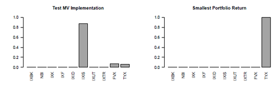
Solution of the MV portfolio with the equally weighted portfolio return as target return, on the left, and with the smallest mean return as target return, on the right.
> barplot(w, ylim = c(0, 1), las = 2,
+ main = "Test MV Implementation")
Another possible test of our implementation involves testing to see that when we set the target return as the smallest possible mean asset return, the entire allocation is assigned to this asset. In our case, the asset that has the smallest mean return is TYX. As shown in the next code snippet and in Figure 13.2, on the right, the optimized portfolio is fully invested in the asset that yields the smallest return:
> w <- MV_QP(x, min(colMeans(x)))
> barplot(w, ylim = c(0, 1), las = 2,
+ main = "Smallest Portfolio Return")
Note that the constraints are passed using the cstr argument or the three dots arguments. Thus, additional constraints can now be easily added to the MV portfolio. For example, the following code snippet illustrates how the budget constraints defined in the previous section can be added to the optimization problem.
> w <- MV_QP(x, mean(x), Sigma = covMcd(x)$cov, GroupBudget())
> barplot(w, ylim = c(0, 1), las = 2,
+ main = "MV with Budget Constraints")
The solution of the MV portfolio with group and budget constraints is displayed in Figure Figure 13.4, on the left.
13.5.3 Robust Mean-Variance Portfolio
A frequently cited drawback of the MV portfolio model is the use of the covariance matrix to estimate risk. The problem resides in the fact that the sample covariance estimator is sensitive to outliers. However, outliers frequently appear in financial data. Because we pass the covariance estimate as an argument to the MV_QP() function, we can easily modify the MV portfolio by using a robust covariance estimator; in this chapter, we use the covMcd() function from the robustbase (Rousseeuw et al. (2012)) package, which implements the fast minimum covariance determinant method given in Rousseeuw & Driessen (1999). Taking the equally weighted portfolio return as the target return, the robust covariance estimator can be used as in the following code snippet:
> w1 <- MV_QP(x, mean(x), Sigma = cov(x))
> barplot(w1, ylim = c(0, 1), las = 2,
+ main = "MV with classical cov")
> w2 <- MV_QP(x, mean(x), Sigma = covMcd(x)$cov)
> barplot(w2, ylim = c(0, 1), las = 2,
+ main = "MV with robust cov")
Figure 13.3 shows the weights obtained with both the classical and robust covariance estimators.

13.5.4 Minimum Variance Portfolio
Use of the mean return has been cited as another drawback of the MV portfolio model. It has been shown that the error in the mean estimator can suppress any benefits from optimization, in which case the optimized weights can produce an inappropriate portfolio on account of the error introduced by potential outliers that influence the estimation of the mean. In this regard, one might wish to consider only the minimum variance portfolio in the absence of a target return, which can be easily implemented by removing the target return condition from the constraints of the portfolio, using
> w <- MV_QP(x, cstr = c(fullInvest(x), longOnly(x)))
> barplot(w, ylim = c(0, 1), las = 2,
+ main = "Minimum Variance Portfolio")
The resultant plot is displayed in Figure 13.4, on the right.
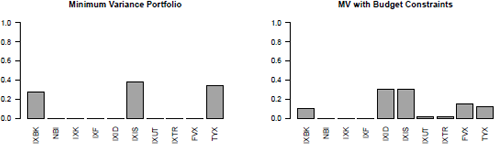
Solution of the MV portfolio with budget constraints, on the left, and of the minimum variance portfolio, on the right.
13.5.5 Conditional Value-at-Risk Portfolio
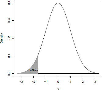
Alternative measures of risk have been introduced in addition to the covariance matrix. One popular risk measure is the so-called Value-at-Risk (VaR) measure. The VaR, which is widely used to measure the risk of loss of a portfolio, defines the loss threshold that might be exceeded for a given probability level. For example, a 5% VaR on a $1000 portfolio indicates a 0.05 probability of a loss of $1000 or more. In statistical terms, the VaR corresponds to a quantile of the portfolio distribution. For example, if P denotes the probability function of X,
VaRα(L)=inf{l∈ℝ: P(l)≥α}
gives the value-at-risk of the portfolio. Figure 13.5 illustrates the 5% value-at-risk of a probability density function.
The drawback of the VaR is that it does not give any information about the maximum loss that can be expected when the VaR has been exceeded, which is especially critical for financial returns that might exhibit a heavy-tailed distribution. The conditional value-at-risk (CVaR), which was introduced as a modification of the VaR, consists of taking the weighted average between the VaR and the losses exceeding the VaR. The CVaR is the conditionally expected value of the loss under the condition that the VaR has been exceeded. The CVaR can be defined as
CVaRα= 11−β∫vaRα(β)f(w,x)f(w,x)p(w,x)dx,
where VaRα is the value-at-risk, f (w, x) is a loss function defined for the portfolio allocation w and the value of the portfolio components, and p is the probability distribution of the portfolio with weights w. In contrast to the VaR, the CVaR is a coherent risk measure, as explained by Artzner et al. (1999). A coherent risk measure is one that satisfies the properties of translation invariance, subadditivity, monotonicity, and positive homogeneity. These properties can be understood in terms of risk measure p on some assets X. Positive homogeneity corresponds to the fact that when the dataset is weighted by a given factor, the risk measure is also weighted according to ρ(λX) =λρ(X) . The subadditivity condition specifies that for two assets X1 and X2 , the risk associated with both assets combined is less than or equal to the sum of the individual risks, according to ρ(X1+X2) ≤ρ(X1)+ρ(X2) . The translation invariance specifies that adding a risk-free asset to the initial portfolio position decreases the risk measure, according to ρ(X+αr)=ρ(X)−α . The monotocity condition specifies that for all X and Y, where X≤Y , the risk of X is less than or equal to the risk of Y, according to ρ(X)≤ρ(Y) .
Initially, the portfolio measure based on the CVaR yields a nonlinear programming problem. However, Uryasev & Rockafellar (2001) showed how to transform the solution into a linear programming problem. The beauty of their approach was to move the VaRa from the boundaries of the integral into the equation, thus adding it as a new parameter to the optimization problem. The transformed problem then becomes
F(X, VaR)=VaR+11−L∫f(w,x)≥VaR(f(w,x)−VaR)p(w,x)dx,
which is equivalent to the CVaR when F is minimized (min F = CVaR). The next step is to note that, given the integral boundary conditions, the element (f(w,x)−α) must be positive. The problem can therefore be transformed to the more general problem in which only positive parts are considered:
VaR+11−L∫x(f(w,x)−VaR)+p(w,x)dy. (13.5)
Scenario-based portfolios represent a large class of portfolios for which the CVaR is an illustrative example. In practice, the scenarios can be obtained using actual portfolio returns or returns obtained by simulation, such as by Monte Carlo simulation. The integral can be approximated using the portfolio returns xt as
≈1j∑Jj=1(f(w,x)−VaR)+.
Linearization of Equation (13.5) can now be performed, where (f(w,xi)−VaR)+ is the nonlinear part of the equation. The linearization consists of adding the new variables zi=(f(w,xi)−Var) to the objective function and adding new constraints to ensure that the optimized zopti are equal to the intended (f(w,xi)−VaR)+ , thus yielding the programming problem
minimizewα+1(1−β)J∑Ji=1Zjsubject toZj≥f(w,xj)−α,(Z1)Zj≥0,(Z2)(13.5)wTˆμ=ˉx,(R)wT1=1,(F)w≥0(L)
Addition of the target return, long only, and full investment conditions then gives the standard CVaR portfolio model. Linearization of the CVaR portfolio consists of the introduction of J +1 additional variables (VaRα and zj) and 2J linear constraints to the optimization problem. Using the linear programming formulation defined in Equation (13.1), we obtain the objective coefficients
c=[ω1ω2⋮ωnαz1z2⋮zn]}N}1}J.
The number of linear constraints in the CVaR portfolio model are therefore becoming sensitively larger than those in the other models described thus far. Because the number of unknown vectors has been increased and the CVaR problem has been linearized, it is now necessary to express the full investment, long only, and other constraints. The equality linear constraints (F and R in Equation (13.6)) for the full investment and target return become, in terms of the new unknown vectors,
Aeq=[N︷11...1w1w2...wn1︷00J︷00...000...0], aeq=[1r] (F)(R)
The inequality linear constraints (Z1 and Z2 in Equation (13.6)), with the long only (L) constraints, become
A=N︷1︷J︷[x11x21⋮xj1x12x22⋮xj2⋯⋯⋱⋯x1nx2n⋮xjn 1 1 ⋮ 111⋱1_11⋱ 1_11⋱1], a=[__]}}}J (Z1)J (Z1)N (L)
where missing entries are equal to zero.
When the integral in Equation (13.5) is approximated using a simulation approach, the number of optimized variables and the size of the matrix for the linear constraints can become very large. However, the constraint matrix is mainly filled with zeros, and can be represented by sparse matrices. A common approach for storage of sparse matrices is the triplet representation, in which each non-zero value is stored with its row and column indices.
Given the matrix representation, the typical linear algebraic routine can be implemented to take advantage of the new representation. The recommended R packages for sparse matrices are Matrix (Bates & Maechler (2012)) and the alternative package slam (Hornik et al. (2013)), both of which are supported by the linear programming package Rglpk used in this chapter.
The following code snippet implements the linearized CVaR portfolio problem (note the use of sparse matrices for constructing the constraint matrix):
> CVaR_LP <- function(x, target, alpha = 0.95, ...,
+ cstr = c(fullInvest(x),
+ targetReturn(x, target),
+ longOnly(x)),
+ trace = FALSE) {
+
+ # number of scenarios
+ J <- nrow(x)
+
+ # number of assets
+ size = ncol(x)
+
+ # objective coefficients
+ c_weights <- rep(0, size)
+ c_VaR <- 1
+ c_Scenarios <- rep(1 / ((1 - alpha) * J), J)
+ c <- c(c_weights, c_VaR, c_Scenarios)
+
+ # extract values from constraint to extend them
+ # with CVaR constraints
+ Aeq <- Reduce(rbind, cstr[names(cstr) %in% "Aeq"])
+ aeq <- Reduce(c, cstr[names(cstr) %in% "aeq"])
+ A <- Reduce(rbind, cstr[names(cstr) %in% "A"])
+ a <- Reduce(c, cstr[names(cstr) %in% "a"])
+
+ # build first two blocks of the constraint matrix
+ M1 <- cbind(Aeq, simple_triplet_zero_matrix(nrow(Aeq), J + 1))
+ M2 <- cbind(A, simple_triplet_zero_matrix(nrow(A), J + 1))
+
+ # identity matrix and vector of zeros
+ I <- simple_triplet_diag_matrix(1, J)
+
+ # block CVaR constraint (y x + alpha + z_j >= 0)
+ M3 <- cbind(x, rep(1, J), I)
+
+ # block CVaR constraint (z_j >= 0)
+ M4 <- cbind(simple_triplet_zero_matrix(J, size +1), I)
+
+ # vector of zeros used for the rhs of M3 and M4
+ zeros <- rep(0, J)
+
+ # combine constraints
+ cstr <- list(Aeq = M1,
+ aeq = aeq,
+ A = rbind(M2, M3, M4),
+ a = c(a, zeros, zeros))
+
+ # optimization
+ sol <- LP_solver(c, cstr, trace = trace)
+
+ # extract weights
+ weights <- sol$solution[1:size]
+ names(weights) <- colnames(x)
+
+ # extract VaR and CVaR
+ VaR <- sol$solution[size + 1]
+ CVaR <- c(c sol$solution)
+ attr(weights, "risk") <- c(VaR = VaR, CVaR = CVaR)
+
+ weights
+}
In the next code snippet, we optimize the weights that minimize the CVaR measure with α=0.05 using the equally weighted portfolio return (mean(x)) as the target return:
round(CVaR_LP(x, mean(x)), 3)
IXBK NBI IXK IXF IXID IXIS IXUT IXTR FVX TYX
0.050 0.000 0.000 0.000 0.026 0.822 0.000 0.000 0.051 0.052
attr(,"risk")
VaR CVaR
0.01081098 0.01363397
The CVaR_LP returns the optimized weights together with the estimated VaR and CVaR.
13.5.6 Minimum Drawdown Portfolio
Only linear constraints have been introduced thus far. However, in some instances, portfolio allocation models may require nonlinear constraints. For example, an investor might be interested in minimizing the maximum drawdown of his portfolio. The drawdown rate of financial instruments at time t corresponds to the rate between the value of the instrument at time t and the latest historical peak:
D(t)=(Pt−maxi∈(1,t)Pi)/maxi∈(1,t)Pi.
Historical peaks can be calculated in R using the cumulative maximum function cummax(); thus, the cumulative peaks for the IXBK index can obtained using the following code snippet and result is displayed in Figure 13.6, on the left:

Historial peaks of the IXBK index, on the left, and drawdown rates for the IXBK index, on the right.
> plot(prices$Date, cummax(prices$IXBK), type = "l",
+ xlab = "Date", ylab = "Cumulative Maximum",
+ main = "Historical Peaks")
Because the returns have already been determined in the previous portfolio optimization problem, the following code snippet implements the drawdown rate from these returns:
> drawdown <- function(x) {
+ value <- cumprod(c(1, 1 + x))
+ cummaxValue <- cummax(value)
+ (value - cummaxValue) / cummaxValue
+}
Figure 13.6, on the right, illustrates the drawdown rate for the IXBK index and was created with the next code snippet:
> plot(prices$Date, drawdown(x[, "IXBK"]), type = "l",
+ xlab = "Date", ylab = "Drawdowns of IXBK",
+ main = "Max Drawdowns")
13.6 Display Results
13.6.1 Efficient Frontier
The usual approach for comparing the feasibility of different portfolios with a given set of assets is the so-called efficient frontier approach, which consists of comparing reward measures and risk measures for different feasible sets of asset weightings.
The following example shows, step-by-step, the method to construct the efficient frontier for an MV portfolio. A straightforward approach is to set a target risk measure and maximize the reward measure. However, in Section 13.5.2, we have implemented the MV portfolio as a quadratic programming problem in which the risk measure is minimized for a given level of reward. Given this formulation, we can minimize the variance of the portfolio for the range of feasible returns of the portfolio. When considering long only positions, the feasible portfolio returns range from the smallest to the largest returns of the portfolio constituents. We set the range of feasible returns of the portfolio as
> mu <- apply(x, 2, mean)
> reward <- seq(from = min(mu), to = max(mu), length.out = 300)
> sigma <- apply(x, 2, sd)
The respective MV portfolios can now be calculated over different return steps. In this example we selected 300 steps so as to achieve a nicely smoothed efficient frontier. Using the function we implemented in Section 13.5.2, we obtain
> Sigma <- cov(x)
> riskCov <- sapply(reward, function(targetReturn) {
+ w <- MV_QP(x, targetReturn, Sigma)
+ sd(c(x %*% w))
+})

Two points are noteworthy in the previous R snippet. First, the covariance matrix was precalculated and passed to the quadratic optimization problem; this is important from a computational point of view, as otherwise the covariance matrix would be recalculated 300 times, which would increase the processing time. Second, we returned the standard deviation, as this is the measure we have selected for the efficient frontier; this is important if one wishes to compare the efficient frontiers of portfolios optimized with different types of covariance matrices.
The efficient frontier can now be plotted together with the locations of the individual asset returns, using
> xlim <- range(c(sigma, riskCov), na.rm = TRUE)
> ylim <- range(mu)
> plot(riskCov, reward, type = "l", xlim = xlim, ylim = ylim,
+ xlab = "Risk", ylab = "Reward",
+ main = "Efficient Frontier")
> points(sigma, mu, col = "steelblue", pch = 19, cex = 0.8)
> text(sigma, mu, labels = colnames(x), pos = 2, cex = 0.8)
13.6.2 Weighted Return Plots
In addition to the efficient frontier, the weighted return plot is another common approach for comparing the weights of feasible portfolio sets. The principle of the weighted return plot is to compare the weight diversifications of the different target reward or risk measures.
Weight plots can constructed in R using the barplot() function. The matrix weights calculated in the previous section can be passed as the first argument, and each set of weights is then represented by stacked sub-bars, which together make up a single histogram bar. The following code snippet implements a simple weighted return plot:
> weightbarplot <- function(weights,
+ title = "Weighted Return Plot") {
+
+ # color palette
+ size <- nrow(weights)
+ col <- gray(seq(size) / (size +1))
+
+ # Bar plot
+ len <- ncol(weights)
+ h <- barplot(weights, space = 0, border = col, col = col,
+ xlim = c(0, len * 1.2), main = title)
+ idx <- seq(1, len, length.out = 5)
+
+ # Reward label
+ mtext("Reward Target", side = 1, line =2, at = mean(h))
+ axis(1, at = h[idx], labels = signif(reward[idx], 2),
+ cex = 0.6)
+
+ # Weight label
+ mtext("Weight", side = 2, line = 2)
+
+ # legend
+ legend("topright", legend = rownames(weights), bty = "n",
+ fill = col)
+}
The most important part of the code is the call to the barplot() function and the passing of the weights matrix as the first argument. The remainder of the code only adds cosmetic improvements to the default barplot() settings. Note that the gray function generates a palette of gray levels, based on the number of assets in the portfolio basket. The use of a consistent and pleasing palette (and one that represents a corporation's color palette) is critical for the generation of effective and professional reports.
Given that the R function has been implemented to construct the weighted return plot, we can compare, for example, the weighted diversification of the MV portfolio implemented in Section 13.5.2 using the classical and robust covariance estimators. The following two snippets estimate the set of weights along the range of feasible target returns. The weighted return of the MV portfolio with the classical covariance estimator is calculated as
> Sigma <- cov(x)
> weightsCov <- sapply(reward, function(targetReturn) {
+ MV_QP(x, targetReturn, Sigma)
+})
> weightbarplot(weightsCov,
+ title = "Weighted Return Plot (Sample Cov)")
and the one with the robust covariance estimator is
> SigmaRob <- covMcd(x)$cov
> weightsRob <- sapply(reward, function(targetReturn) {
+ MV_QP(x, targetReturn, SigmaRob)
+})
> weightbarplot(weightsRob,
+ title = "Weighted Return Plot (Robust Cov)")
The resultant graphics are displayed in Figure 13.8.

Weighted return plots of the MV portfolio using the sample and robust covariance estimator.
13.7 Conclusion
This chapter described the basic elements of portfolio optimization for problems consisting of minimizing a risk measure under a given set of constraints. The examples were constructed in such a way that they can be extended to more advanced and complex situations. However, the reader should bear in mind that a large number of portfolio models exist that have not been described in this chapter. For example, the extension of the Black-Litterman approach by Meucci, known as the entropy polling approach, is an interesting method for combining information extracted from historical data with forecasts from analysts. Moreover, other types of measures are available, such as the divergence measure from information theory, as introduced in Chalabi (2012).
Finally, it is important to point out that the choice of optimization routine can have an important impact on the optimized weights. We encourage practitioners to compare and choose optimization algorithms that are most appropriate for their portfolio problems. In this regard, an interesting approach to the comparison of several optimization routines that interface with R is by using the programming language AMPL, which offers a common interface for a large set of free and commercial solvers.
Good sources of information for portfolio optimization in R are the works of Würtz et al. (2009) from the Rmetrics Association, and the work of Pfaff (2012), in which readers are guided in a step-by-step approach to portfolio solvers in R; the works are accompanied by the packages fPortfolio and FRAPO, respectively.
In addition, BLCOP, see Gochez (2011), is an implementation of the Black-Litterman model and Meucci's copula opinion pooling framework; PerformanceAnalytics (Carl & Peterson (2013)) provides numerous econometric tools for performance and risk analysis; the package backtest Enos, Kane, with contributions from Kyle Campbell, Gerlanc, Schwartz, Suo, Colin, & Zhao (2012) provide facilities for exploring portfolio-based conjectures about financial instruments (stocks, bonds, swaps, options, etc.); crp.CSFP (Jakob et al. (2013)) implements the program CreditRisk+ (see Boston (1997)); parma, see Ghalanos (2013), implements portfolio allocation and risk management applications; portfolioSim, see Enos, Kane & with contributions from Kyle Campbell (2012b), is a framework for simulating equity strategies; portfolio (Enos, Kane, with contributions from Daniel Ger- lanc & Campbell (2012)) provides R classes for analyzing and implementing equity portfolios; rportfolios (Novomestky (2012)) offers functions to generate random portfolios; stockPortfolio, see Diez & Christou (2012), can be used to build stock models and analyze stock portfolios; and tawny, see Rowe (2013), applies random matrix theory and the shrinkage estimator to portfolio problems.