
Chapter 1
Introduction
Arthur Charpentier
Université du Québec à Montréal
Montréal, Québec, Canada
Rob Kaas
Amsterdam School of Economics, Universiteit van Amsterdam
Amsterdam, Netherlands
1.1 R for Actuarial Science?
As claimed on the CRAN website, http://cran.r-project.org/, R is an “open source software package, licensed under the GNU General Public License” (the so-called GPL). This simply means that R can be installed for free on most desktop and server machines. This platform independence and the open-source philosophy make R an ideal environment for reproducible research.
Why should students or researchers in actuarial science, or actuaries, use R for computations? Of primary interest, as suggested by Daryl Pregibon, research scientist at Google— quoted in Vance (2009)—is that R “allows statisticians to do very intricate and complicated analyses without knowing the blood and guts of computing systems.”
In this chapter, we will briefly introduce R, compare it with other standard programming languages, explain how to link R with them (if necessary), give an overview of the language, and show how to produce graphs. But as stated in Knuth (1973), “premature optimization is the root of all evil (or at least most of it) in programming,” so we will first describe intuitive (and hopefully easy to understand) algorithms before introducing more efficient ones.
1.1.1 From Actuarial Science to Computational Actuarial Science
In order to illustrate the importance of computational aspects in actuarial science (as introduced in the preface), consider a standard actuarial problem: computing a quantile of a compound sum, such as the 99.5% quantile (popular for actuaries dealing with economic capital, and the Value-at-Risk concept). There exists an extensive literature on computing the distribution in collective risk models. From a probabilistic perspective, we have to calculate, for all s ∈ ℝ,
F(s)=ℙ(S≤s),where S=N∑i=1Xi.
By independence, a straightforward convolution formula (see e.g. Chapter 3 in Kaas et al. (2008)) can be used:
F(s)=∞∑n=0F*nX(x).ℙ(N=n).
From a statistician's perspective, the distributions of N and Xi are unknown but can be estimated using samples. To illustrate the use of R in actuarial science, consider the following (simulated) sample, with 200 claims amounts
> set.seed(1)
> X <- rexp(200,rate=1/100)
> print(X[1:5])
[1] 75.51818 118.16428 14.57067 13.97953 43.60686
From now on, forget how we generate those values, and just keep in mind that we have a sample, and let us use statistical techniques to estimate the distribution of the Xi ’s. A standard distribution for loss amounts is the Gamma(α, β) distribution. As we will see in Chapter 2, other techniques can be used to estimate parameters of the Gamma distribution, but here we can solve the normal equations, see for example Section 3.9.5 in Kaas et al. (2008). They can be written as
logˆα−Γ′(ˆα)Γ(ˆα)−logˉX+¯logX=0 and ˆβ=ˆαˉX.
To solve the first equation, Greenwood & Durand (1960) give tables for ˆα as a function of M=logˉX−¯logX, as well as a rational approximation. But using the digamma function Γ′(α)/Γ(α), nowadays solving it is a trivial matter, by means of the function uniroot(). This goes as follows:
> f <- function(x) log(x)-digamma(x)-log(mean(X))+mean(log(X))
> alpha <- uniroot(f,c(1e-8,1e8))$root
> beta <- alpha/mean(X)
We now have a distribution for the Xi's. For the counting process, assume that N has a Poisson distribution, with mean 100. A standard problem is to compute the quantile with probability 99.5% (as requested in Solvency II) of this compound sum. There are hundreds of academic articles on that issue, not to mention chapters in actuarial textbooks. But the computational aspect of this problem can actually be very simple. A first idea can be to compute numerically the sum (with a given number of terms) in the convolution formula above, using that a sum of independent Gamma random variables still has a Gamma distribution,
> F <- function(x,lambda=100,nmax=1000) {n <- 0:nmax
+ sum(pgamma(x,n*alpha,beta)*dpois(n,lambda))}
Once we have a function to compute the cumulative distribution function of S, we just need to invert it. Finding x such that F(x)=.995is the same as finding the root of function x↦F(x)−.995
> uniroot(function(x) F(x)-.995,c(1e-8,1e8))$root
[1] 13654.43
A second idea can be to use fast Fourier transform techniques, since it is (at least from a theoretical perspective) much more convenient to use the generating function when computing the distribution of a compound sum, if we use a discretized version of Xi’s. Here the code to compute the probability function of S (after discretizing the Gamma distribution, on ℕ = {0, 1, 2, . . .}, with an upper bound, here 220) is simply
> n <- 2^20; lambda <- 100
> p <- diff(pgamma(0:n-.5,alpha,beta))
> f <- Re(fft(exp(lambda*(fft(p)-1)),inverse=TRUE))/n
This is possible because R has a function, called fft(), to compute either the Fourier transform, or its inverse. To compute the quantile of level α, we just have to find xα such that F(xα−1)<α≤F(xα) (since we use a discretization on ℕ). The R code to compute that value is
> sum(cumsum(f)<.995)
[1] 13654
All those methods will be discussed in Chapter 2. The point here was to prove that using an appropriate computational language, many actuarial problems can be solved easily, with simple code. The most difficult part is now to understand the grammar of the R language.
1.1.2 The S Language and the R Environment
R is a scripting language for data manipulation, statistical analysis and graphical visualization. It was inspired by the S environment (the letter S standing for statistics), developed by John Chambers, Douglas Bates, Rick Becker, Bill Cleveland, Trevor Hastie, Daryl Pregibon and Allan Wilks from the AT&T research team in the 1970s. In 1998 the Association for Computing Machinery (ACM) gave John Chambers the Software System Award, for “the S system, which has forever altered the way people analyze, visualize, and manipulate data.”
R was written by Ross Ihaka and Robert Gentleman, at the Department of Statistics of the University of Auckland. John Chambers contributed in the early days of Rand later became a member of the core team. The current R is the result of a collaborative project, driven by this core team, with contributions from users all over the world.
R is an interpreted language: when expressions are entered into the R console, a program within the R system (called the interpreter) executes the code, unlike C/C++ but like JavaScript (see Holmes (2006) for a comparison). For instance, if one types 2+3 at the command prompt and presses Enter, the computer replies with 5. Note that it is possible to recall and edit statements already typed, as R saves the statements of the current session in a buffer. One can use the ↑ and the ↓ keys either to recall previous statements, or to move down from a previous statement. The active line is the last line in the session window (called console), and one can use the ← and the → keys to move within a statement in this active line. To execute this line, press Enter .
In this book, illustrations will be based on copies of the console. Of course, we strongly recommend the use of an editor. The user will type commands into the editor, select them (partially or totally), and then run selected lines. This can be done in press Windows RGui, via File and New script menu (or Open script for an existing one). The natural extension for R script is a .R file (the workspace will be stored in a .RData file, but we will get back to those objects later on). It is also possible to use any R editor, such as RStudio, Tinn-R or JGR (which stands for Java Gui for R). In all the chapters of this book, R codes will be copies of prompts on the screen: the code will follow the > symbol (or the + symbol when the command is not over). If we go back to the very first example of this book, in the script file there was
set.seed(1)
X <- rexp(200,rate=1/100)
print(X[1:5])
If we select those three lines and press Run, the output in the console is
> set.seed(1)
> X <- rexp(200,rate=1/100)
> print(X[1:5])
[1] 75.51818 118.16428 14.57067 13.97953 43.60686
To go further, R is an Object-Oriented Programming language. The idea is to create various objects (that will be described in the next sections) that contain useful information, and that could be called by other functions (e.g. graphs). When running a regression analysis with SAS® or SPSS®, output appears on the screen. By contrast, when calling the lm regression function in R, the function returns an object containing various information, such as the estimated coefficients ˆβ, the implied residuals ˆε, estimated variance matrix of the coefficients var(ˆβ), etc. This means that in R, the analysis is usually done in a series of consecutive steps, where intermediate results are stored in objects. Those objects are then further manipulated to obtain the information required, using dedicated functions. As we will see later (in Section 1.2.1), “everything in S is an object,” as claimed in the introduction of Chapter 2 of Venables & Ripley (2002). Not only are vectors and matrices objects that can be passed to and returned by functions, but functions themselves are also objects, even function calls.
In R, the preferred assignment operator (by the user community) is the arrow made from two characters <-, although the symbol = can be used instead. The main advantage of the <- is that it allows one to assign objects within a function,. For instance
> summary(reg <- lm(Y~X1+X2))
will not only print the output of a linear regression, but will also create the object reg. Again, Section 1.2 will be dedicated to R objects.
An mentioned previously, in this book, R code will follow the > symbol, or the + symbol when the line is not over. In R, comments will follow the # tag (everything after the # tag will not be interpreted by R).
> T <- 10 # time horizon
> r <- .05 # discount rate = 5%
> (1+r)^(-
+ T) # 1$ in T years
[1] 0.6139133
R computations will follow the [1] symbol. Observe that it is possible to use spaces. It might help to read the code,
> (1 + r)^(-T)
[1] 0.6139133
and it will not affect computations (unless we split operators with a space; for instance, <- is not the same as < - : just compare x<-1 and x< -1 if you are not convinced). We also encourage the use of parentheses (or braces, but not brackets, used to index matrices) to get a better understanding.
> {1+r}^(-T)
[1] 0.6139133
If you are not convinced, try to understand what the output will be
> -2 ^ .5
It is also possible to use a ; to type two commands on the same line. They will be executed as if they were on two different lines.
> {1+r}^(-T); {1+r/2}^(-T)
[1] 0.6139133
[1] 0.7811984
As mentioned previously, instead of typing code in the console, one can open a script window, type a long code, and then run it, partially or totally. It is also possible to load functions stored in a text file using the source() function:
> source("Rfunctions.txt")
1.1.3 Vectors and Matrices in Actuarial Computations
The most common objects in R are vectors (vectors of integers, reals, even complex, or TRUE-FALSE boolean tests). Vectors can be used in arithmetic expressions, in which case the operations are performed element by element: a*b will return the vector [ai · bi]. In actuarial science, most quantities are either vectors or matrices. For instance, the probability that a person aged x will be alive at age x + k is kpx , which is a function of x and k (both integers) and can be stored in a matrix p. Then any actuarial quantity can be computed using matrix arithmetics. For instance, the curtate expectation of life, given by
ex=∞∑k=1pkx,
can be computed using
> life.exp <- function(x){sum(p[1:nrow(p),x])}
Several actuarial activities (from ratemaking to claims reserving) are simply using past data to create models that should describe future behavior. A set of techniques, called predictive modeling, became widespread among actuaries. The goal is to infer from the data some factors that better explain the risk, in order to compute the premium for different policyholders, or to calculate reserves for different types of claims. As we will see, using dedicated functions on those data, it will be possible to compute any actuarial quantity. But before discussing datasets, let us spend some time on coding functions in R.
1.1.4 R Packages
A package is a related set of functions, including help files and data files, that have been bundled together and is shared among the R community. Those packages are similar to libraries in C/C++ and classes in Java. To get the list of packages loaded by default, the getOption command can be used:
> getOption("defaultPackages")
[1] "datasets" "utils" "grDevices" "graphics" "stats" "methods"
> (.packages(all.available=TRUE))
[1] "AER" "evd" "sandwich" "lmtest" "nortest"
and many more packages, previously installed on the machine. All these packages are available; you just have to load them. But before, we have to install a package from the Internet (for instance quantreg to run quantile regressions) we use
> install.packages("quantreg", dependencies=TRUE)
and then we select a mirror site to download. The option dependencies=TRUE is used because the quantreg package might be using functions coming from other packages (here, the MatrixModels package has to be installed too). See Zhang & Gentleman (2004) for interactive exploration of R packages. Note that if a package has not been loaded, it is not possible to call associated functions:
> fit <- rq(Y ~ X1 + X2, data = base, tau = .9)
Error: could not find function "rq"
To load a package in R, one should use either the library() command, or the require() one,
> library(quantreg)
As mentioned in Fox (2009), the number of packages on CRAN has grown roughly exponentially, by almost 50% each year (this was confirmed on updated counts). With thousands of packages, inevitably, functions with similar names can be loaded. For instance, the default stats4 package (containing statistical functions related to the S4 class that will be discussed in the next paragraph) contains a coef function,
> coef
function (object, ...) UseMethod("coef")
<bytecode: 0x16d1d80>
<environment: namespace:stats>
Note the use of ellipsis (...) in the function. This is an interesting feature of R-functions, that allows functions to have a variable number of arguments. But a function with the same name exists in the VGAM package (for additive models, see Yee (2008))
> library(VGAM)
The following object(s) are masked from ’package:stats4’:
coef
Now function coef will be called from this package,
> coef
standardGeneric for "coef" defined from package "VGAM"
function (object, ...)
standardGeneric("coef")
<environment: 0x2981fcb0>
Methods may be defined for arguments: object
Use showMethods("coef") for currently available ones.
If the VGAM package is loaded, and we need to run function coef() from library stats4, it is either possible to unload it, using
> detach(package:VGAM, unload=TRUE)
or to call the function using stats4::coef.
Finally, observe that packages are regularly updated. In order to run the latest version, it might be a good thing to run, frequently, the following line
> update.packages()
The update should be run before loading packages, and one should keep in mind that updates might be possible only on the latest version of R (see Ripley (2005) for a discussion). It is also possible to get an overview of existing packages on different topics on the task views page, see http://cran.r-project.org/web/views/, such as empirical finance or computational econometrics (see Zeileis (2005) for additional information).
Another difficult task, for new users, is to find which package will be appropriate to deal with a specific problem. Consider the problem of longitudinal mixed models (developed in Chapter 15). Consider the following hierarchical model
Yi=β1Xi+γ0+γ1Zj[i]+uj[i]︸random component aj[i]+εi,
where individual i belongs to a group (company, region, car type, etc.) j. Several packages can be used to deal with this model, or more generally nonlinear mixed-effect models, such as nlme or lme4. One can also use plm for panel regression models. At least two functions can be used to estimate the model above, lme() and lmer(). More details about function lmer() can be found in Bates (2005), and from linear and nonlinear mixed effects models described in Pinheiro & Bates (2000). For instance, to run a regression, use either
> reg <- lme(fixed = Y ~ X, random = ~ X | Z, method=’ML’)
or
> reg <- lmer(Y ~ X+ Z + (1 | Z), method=’ML’)
Note that the syntax can be different, as well as the output. Gelman & Hill (2007) suggest the use of lmer() for instance, as lme() only accepts nested random effects, while lmer() handles crossed random effects. On the other hand, lme() can handle heteroscedasticity (while lmer() does not). Further, lme() returns p-values, while lmer() does not. Choosing a package is not a simple task.
1.1.5 S3 versus S4 Classes
In order to get a good understanding of R functions and packages, it is necessary to understand the distinction between S3 and S4 classes. The basic difference is that S3 objects were created with an old version of R (or S, the so-called third version), while S4 objects were created with a more recent version of R (or S, the so-called fourth version). But it is still possible to create S3 objects with the latest version of R. For example, in regression models, lm, glm and gam are S3 objects, while lmer (for mixed effects models) and VGAM (for vector generalized linear and additive models) are S4. See Bates (2003) for a discussion about those two classes.
To illustrate the distinction between the two, consider the case of health insurance, where we have characteristics of some individuals. It is possible to define a person object that will contain all important information. And then we can define functions on such an object.
S3 is a primitive concept of classes, in R. To define a class that will contain characteristics of a person, use
> person3 <- function(name,age,weight,height){
+ characteristics<-list(name=name,age=age,weight=weight,height=height)
+ class(characteristics)<-"person3"
+ return(characteristics)}
To create a person, we just have to give proper arguments:
> JohnDoe <- person3(name="John",age=28, weight=76, height=182)
> JohnDoe
$name
[1] "John"
$age
[1] 28
$weight
[1] 76
$height
[1] 182
attr(,"class")
[1] "person3"
Observe the use of the $ symbol, to get attributes of that list,
> JohnDoe$age
[1] 28
Then it is possible to define a function on a person3 object. If we want a function that returns the BMI (Body Mass Index), use
> BMI3 <- function(object,...) {return(object$weight*1e4/object$height^2)}
Then, we can call that function on JohnDoe
> BMI3(JohnDoe)
[1] 22.94409
As mentioned in the previous paragraph, lm objects are in the S3 class.
> reg3 <- lm(dist~speed,data=cars)
> reg3$coefficients
(Intercept) speed
-17.579095 3.932409
> coef(reg3)
(Intercept) speed
-17.579095 3.932409
> plot(reg3)
Note that with S3 objects, a function is usually defined with a certain list of arguments (see the lm function), and then to define a generic function, there is a UseMethod call with the name of the generic function. For example, the generic summary
> summary
function (object, ...) UseMethod("summary")
<environment: namespace:base>
The latest version, S4, allows object-oriented programming with S (see Chambers & Lang (2001)). An object is a set (or a list) of functions, and it should be associated with functions dealing with that object. Object programming might appear more complex, as the code should be thought through in advance. As mentioned in Lumley (2004), “as a price for this additional clarity, the S4 system takes a little more planning.”
To create an object, use
> setClass("person4", representation(name="character",
+ age="numeric", weight="numeric", height="numeric"))
[1] "person4"
To create a person, use the new function, for example,
> JohnDoe <- new("person4",name="John",age=28, weight=76, height=182)
> JohnDoe
An object of class "person"
Slot "name":
[1] "John"
Slot "age":
[1] 28
Slot "weight":
[1] 76
Slot "height":
[1] 182
Attributes of those objects are obtained using the @ symbol (and no longer the $)
> JohnDoe@age
[1] 28
Then, it is possible to define functions on those objects, for example, to compute the BMI. The first argument will be the name of the function (here BMI4), the second one will be the object name (here a person4), and then the code of the function. But first, it is necessary to define the method BMI4 using the setGeneric function
> setGeneric("BMI4",function(object,separator) return(standardGeneric("BMI")))
[1] "BMI4"
> setMethod("BMI4", "person4", function(object){return(object@weight*1e4/object@height^2)})
[1] "BMI4"
Then, we can use this function on all individuals we have,
> BMI4(JohnDoe)
[1] 22.94409
As mentioned previously, VGAM objects are in the S4 class.
> library(VGAM)
> reg4 <- vglm(dist~speed,data=cars,family=gaussianff)
> reg4@coefficients
(Intercept) speed
-17.579095 3.932409
> coefficients(reg4)
(Intercept) speed
-17.579095 3.932409
For those two examples, we can see that S3 and S4 classes are rather similar, and actually, both classes coexist (so far peacefully) in R. See Genolini (2008) for more details, especially on the concept of inheritance that can be used only with S4 classes, Leisch (2009) on R packages or Lumley (2004) which compares ROC curves (defined in Chapter 4) with S3 and S4 classes, respectively.
It is necessary to understand that those two classes both exist, as some libraries use only S3 classes (described in this introductory chapter), while others do use S4, such as several probability distributions used in Chapter 2 (see Ruckdeschel et al. (2006) for a discussion on S4 classes for distributions) or lifetable objects in Chapter 8.
1.1.6 R Codes and Efficiency
In this book, we will discuss computational aspects of actuarial sciences. So there will be a tradeoff between a very efficient code, where the structure of the algorithm might not be explicit, and a simple code, to illustrate how to compute quantities, but which might be quite slow. Efficient techniques will be mentioned in this chapter, and to illustrate efficiency, instead of using flop counting (we might refer to Knuth (1973), Press et al. (2007) or Cormen et al. (1989) for details), we will use R functions that measure how long a particular operation takes to execute, such as system.time, which returns CPU times, and others. For instance, if we consider the product of two matrices 1, 000 × 1, 000,
> n <- 1000
> A <- matrix(seq(1,n^2),n,n)
> B <- matrix(seq(1,n^2),n,n)
> system.time(A%*%B)
user system elapsed
1.040 0.020 1.226
we can see that on a standard machine, it took around 1 second to compute the product (time is here in seconds). And around the same time to see that this matrix could not be inverted
> system.time(solve(A%*%B))
Error in solve.default(A %*% B) :
Lapack routine dgesv: system is exactly singular
Timing stopped at: 1.466 0.069 1.821
For deterministic computations, if we want to compare computation time, use function benchmark from library(rbenchmark)
> benchmark(A*B,A%*%B,replications=1)[,c(1,3,4)]
test elapsed relative
1 A * B 0.006 1.000
2 A %*% B 0.989 164.833
where we can see compare element by element and matrices product computations. In the context of random number generation, it might be interesting to use the library(microbenchmark). Here, based on ten computations of the same quantity,
> microbenchmark(A*B,A%*%B,times=10) Unit: milliseconds
expr min lq median uq max neval
A * B 3.369552 3.49644 3.763942 5.085174 8.988348 10
A %*% B 970.899445 979.78303 994.234688 999.586548 1024.985193 10
Here, on deterministic computations for the matrices product, it took 1 second, each time. Those times might be very different when using Monte Carlo simulations, with much more variability (especially when rejection techniques are used).
1.2 Importing and Creating Various Objects, and Datasets in R
After this general introduction, let us spend some time to discover R’s grammar.
1.2.1 Simple Objects in R and Workspace
As claimed in the introduction of Chapter 2 of Venables & Ripley (2002),
“Everything in S is an object.”
“Every object in S has a class.”
For instance, to assign a value to an object (and to create that object if it does not exist yet), we use the assignment operator <-. Command
> x <- exp(1)
> x
[1] 2.718282
will create a numeric variable denoted x, with value e.
> class(x)
[1] "numeric"
Almost all names can be used, except a small list of taken words, such as TRUE or Inf. The latter is defined such that
> 1/0
[1] Inf
Observe that the largest number (before reaching infinity) is
> .Machine$double.xmax
[1] 1.797693e+308
So here,
> 2e+307<Inf
[1] TRUE
> 2e+308<Inf
[1] FALSE
And finally observe that
> 0/0
[1] NaN
where NaN stands for Not A Number (which makes sense because 0/0 is not properly defined). If pi has a default value when starting R (π, ratio of a circle’s circumference to its diameter, numerically 3.141593 · · · etc.), it is possible to create an object named pi. But it might be a bad idea. Keep in mind also that, when loading R, T and TRUE are equivalent (and so are F and FALSE), which explains why, in some codes, we can find mean(x,na.rm=T), for instance. Nevertheless, we strongly recommend to avoid using T instead of TRUE, and to keep T as a possible variable (that can be used for time). The list of all objects stored in R memory can be obtained using the ls() function. It is possible to define objects x2, x_2, or x.2, but not 2x. Object names cannot start with a numeric value.
Using
> y <- x+1
will create another object, y with value e + 1. From a technical point of view, R uses copying semantics , which makes R a pass by value language: y stores a numeric value and is not a function of x. Thus, if the value of x changes, this will not affect the value of y,
> x <- pi
> y
[1] 3.718282
A numeric class object has values in ℝ, while the class integer refers to values in ℤ. The logical class is for values TRUE and FALSE.
The objects we created can be stored in a file called .RData (in the directory where we started R). Our workspace is one of the several locations where R can find objects.
> find("x")
[1] ".GlobalEnv"
The workspace is just an environment in R (a mapping between names, and values). Note that predefined objects are stored elsewhere
> find("pi")
[1] "package:base"
Objects can be stored in several locations,
> search()
[1] ".GlobalEnv" "tools:RGUI" "package:stats"
[4] "package:graphics" "package:grDevices" "package:utils"
[7] "package:datasets" "package:methods" "Autoloads"
[10]"package:base"
1.2.2 More Complex Objects in R: From Vectors to Lists
1.2.2.1 Vectors in R
The most natural way to define and store more than one value in R is to create a vector, which is probably the simplest R object. This can be done using the c() function (to concatenate or combine)
> x <- c(-1,0,2)
> x
[1] -1 0 2
> y <- c(0,2^x)
> y
[1] 0.0 0.5 1.0 4.0
Here, [1] states that the answer is starting at the first element of a vector: when displaying a vector, R lists the elements, from the left to the right, using (possibly) multiple rows (depending on the width of the display). Observe that if an object is followed by the assignment operator <-, then a value (or a dataframe, or a function, etc.) will be assigned to the object. If we simply type the name of the object, and then Enter, the value of the object will appear in the console (or the code of the function, if the object is a function). Each new row includes the index of the value starting that row, that is,
> u <- 1:50
> u
[1] 1 2 3 4 5 6 7 8 9 10 11 12 13 14 15 16 17
[18] 18 19 20 21 22 23 24 25 26 27 28 29 30 31 32 33 34
[35] 35 36 37 38 39 40 41 42 43 44 45 46 47 48 49 50
Note that there is a NULL symbol in R.
> c(NULL,x)
[1] -1 0 2
Such an object can be useful to create an object used in a loop.
> x <- NULL
> for(i in 1:10){x <- c(x,max(sin(u[1:i])))}
> x
[1] 0.8414710 0.9092974 0.9092974 0.9092974 0.9092974
[6] 0.9092974 0.9092974 0.9893582 0.9893582 0.9893582
We have seen function c(), used to concatenate series of elements (having the same type), but one can also use seq() to generate a sequence of elements evenly spaced:
> seq(from=0, to=1, by=.1)
[1] 0.0 0.1 0.2 0.3 0.4 0.5 0.6 0.7 0.8 0.9 1.0
> seq(5,2,-1)
[1] 5 4 3 2
> seq(5,2,length=9)
[1] 5.000 4.625 4.250 3.875 3.500 3.125 2.750 2.375 2.000
or rep(), which replicates elements
> rep(c(1,2,6),3)
[1] 1 2 6 1 2 6 1 2 6
> rep(c(1,2,6),each=3)
[1] 1 1 1 2 2 2 6 6 6
It is important to keep in mind that R is case sensitive, so x is not the same as X. Observe also that there are no pointers in R. If we use the sort function, it will print the sorted vector. But the order will not change.
> x <- c(-1,0,2)
> sort(x,decreasing=TRUE)
[1] 2 0 -1
> x
[1] -1 0 2
If we want to sort vector x, then we should reassign the vector (which is possible in R),
> x <- sort(x,decreasing=TRUE)
> x
[1] 2 0 -1
Observe that it is possible to assign names to the elements of the vector,
> names(x) <- c("A","B","C")
> x
A B C
-1 0 2
and then components of the vectors can be called using brackets [], with either
> x[c(3,2)]
C B
2 0
or
> x[c("C","B")]
C B
2 0
which is a shorter version for x[names(x)%in%c("C","B")].
With runif(), we can generate random variables, uniformly distributed over the unit interval [0, 1] (most standard distributions can be generated with standard functions in R, as discussed later on in this chapter and in Chapter 2),
> set.seed(1)
> U <- runif(20)
By setting the seed of the generating algorithm, so-called random numbers will always be the same, and we will have examples that can be reproduced.
By default, seven digits are displayed
> U[1:4]
[1] 0.2655087 0.3721239 0.5728534 0.9082078
It is possible to display more digits, or less, by setting the number of digits to print, from
1 to 22:
> options(digits = 3)
> U[1:4]
[1] 0.266 0.372 0.573 0.908
> options(digits = 22)
> U[1:4]
[1] 0.2655086631420999765396 0.3721238996367901563644
[3] 0.5728533633518964052200 0.9082077899947762489319
Only the display is affected, not the way numbers are stored, in R.
R has a recycling rule when working with vectors. The recycling rule is implicit when we use expression x+2, where 2 does not have the size of x. More generally, shorter vectors are recycled as often as needed, until they match the length of the longest one. Hence,
> x <- c(100,200,300,400,500,600,700,800)
> y <- c(1,2,3,4)
> x+y
[1] 101 202 303 404 501 602 703 804
This works also when vector lengths are not multiples,
> y <- c(1,2,3)
> x+y
[1] 101 202 303 401 502 603 701 802
Note that NA values are used to represent missing values, as NA stands for not available
> age <- seq(0,90,by=10)
> length(age) <- 12
> age
[1] 0 10 20 30 40 50 60 70 80 90 NA NA
But R will not always assign values when lengths are not appropriate (and some error message might also appear).
The strength of a vector-based language is that it is very simple to access parts of vectors, specifying subscripts. To return the values of U strictly larger than 0.8, we use
> U[U>.8]
[1] 0.9082078 0.8983897 0.9446753 0.9919061
or if we want value(s) between 0.4 and 0.5,
> U[(U>.4)&(U<.5)]
[1] 0.4976992
Here, a boolean test is made, and the value of U is returned only if the test is TRUE:
> (U>.4)&(U<.5)
[1] FALSE FALSE FALSE FALSE FALSE FALSE FALSE FALSE FALSE
[10] FALSE FALSE FALSE FALSE FALSE FALSE TRUE FALSE FALSE
[19] FALSE FALSE
If the test is FALSE for all components, then a numeric(0) is returned:
> U[(U>.4)&(U<.45)]
numeric(0)
From a mathematical point of view, the set {U > .4} ∩ {U < .45}, here, is empty. Thus, the vector here, two times has a zero length
> length(U[(U>.4)&(U<.45)])
[1] 0
It is also possible to return a vector containing the subscripts of the vector for which the logical test was true:
> which((U>.4)&(U<.6))
[1] 3 16
In order to get the complementary, one can use operators which stands for and, while |
stands for or:
> which((U<=.4)|(U>=.6))
[1] 1 2 4 5 6 7 8 9 10 11 12 13 14 15 17 18 19 20
or one can use the negation operator !
> which(!((U>.4)&(U<.6)))
[1] 1 2 4 5 6 7 8 9 10 11 12 13 14 15 17 18 19 20
For integer values, it is possible to use == to compare values:
> y
[1] 1 2 3 4
> y==2
[1] FALSE TRUE FALSE FALSE
But this symbol can yield tricky situations when comparing non-integers
> (3/10-1/10)
[1] 0.2
> (3/10-1/10)==(7/10-5/10)
[1] FALSE
Those two fractions are not equal, for R, as
> (3/10-1/10)-(7/10-5/10)
[1] 2.775558e-17
In that case, it might be more judicious to use all.equal(),
> all.equal((3/10-1/10),(7/10-5/10))
[1] TRUE
Similarly, (√2)2 is slightly different from 2,
> sqrt(2)^2 == 2
[1] FALSE
To go further on floating-point numbers (that can be represented exactly by a computer), see Goldberg (1991). In R, the smallest positive floating-point number, ∈, such that 1+∈≠1 is
> print(eps<-.Machine$double.eps)
[1] 2.220446e-16
> 1+eps==1
[1] FALSE
It does not mean that R cannot deal with smaller numbers, only that == cannot be used. The smallest number is actually
.Machine$double.xmin
[1] 2.225074e-308
As mentioned earlier, the important idea with vectors is that they are (ordered) collections of elements of the same type, which can be numeric (in ℝ), complex (in ℂ), integer(in ℕ), character for characters or strings, logical, that is FALSE or TRUE (or in {0, 1}). If we try to concatenate elements that are not of the same type, R will coerce elements to a common type, for example,
> x <- c(1:5,"yes")
> x
[1] "1" "2" "3" "4" "5" "yes"
> y <- c(TRUE,TRUE,TRUE,FALSE)
> y
[1] TRUE TRUE TRUE FALSE
> y+2
[1] 3 3 3 2
1.2.2.2 Matrices and Arrays
A matrix is just a vector of data, along with an additional vector, accessible by the dim() function, that contains the dimensions (i.e. number of rows nrow and columns ncol).
> M <- matrix(U,nrow=5,ncol=4)
> M
[,1] [,2] [,3] [,4]
[1,] 0.2655087 0.89838968 0.2059746 0.4976992
[2,] 0.3721239 0.94467527 0.1765568 0.7176185
[3,] 0.5728534 0.66079779 0.6870228 0.9919061
[4,] 0.9082078 0.62911404 0.3841037 0.3800352
[5,] 0.2016819 0.06178627 0.7698414 0.7774452
The dimension of matrix M is obtained using
> dim(M)
[1] 5 4
If we want to reshape the matrix, to get a 4 × 5 matrix, instead of a 5 × 4, it is possible to change the attribute of the object. Here, we can specify ex-post the dimension of the matrix, using
> attributes(M)$dim=c(4,5)
All the elements are sorted the same way (per column), but the matrix has been reshaped,
> M
[,1] [,2] [,3] [,4] [,5]
[1,] 0.2655087 0.2016819 0.62911404 0.6870228 0.7176185
[2,] 0.3721239 0.8983897 0.06178627 0.3841037 0.9919061
[3,] 0.5728534 0.9446753 0.20597457 0.7698414 0.3800352
[4,] 0.9082078 0.6607978 0.17655675 0.4976992 0.7774452
The dimension of matrix M is
> dim(M)
[1] 4 5
Here again, it is possible to use logical subscripts. If we want the lines of M for which the element in the last column is larger than 0.8, we use
> M[M[,5]>0.8,]
[1] 0.37212390 0.89838968 0.06178627 0.38410372 0.99190609
If we want the columns for which the element in the last row is larger than 0.8, we use
> M[,M[4,]>0.8]
[1] 0.2655087 0.3721239 0.5728534 0.9082078
A lot of functions can be used to manipulate matrices. For instance, sweep() can be used to apply a function either to rows (MARGIN=1) or columns (MARGIN=2). For instance, if we want to add i to row i of matrix M, the code will be
> sweep(M,MARGIN=1,STATS=1:nrow(M),FUN="+")
[,1] [,2] [,3] [,4] [,5]
[1,] 1.265509 1.201682 1.629114 1.687023 1.717619
[2,] 2.372124 2.898390 2.061786 2.384104 2.991906
[3,] 3.572853 3.944675 3.205975 3.769841 3.380035
[4,] 4.908208 4.660798 4.176557 4.497699 4.777445
Here, we will (mainly) work with matrices containing numeric values. But it is possible to have matrices of (almost) any format, for instance logical values,
> M>.6
[,1] [,2] [,3] [,4] [,5]
[1,] FALSE FALSE TRUE TRUE TRUE
[2,] FALSE TRUE FALSE FALSE TRUE
[3,] FALSE TRUE FALSE TRUE FALSE
[4,] TRUE TRUE FALSE FALSE TRUE
Observe that the recycling rule of R affects also matrices (a matrix—or an array—being just a rectangular collection of elements of the same type)
> M <- matrix(seq(1,8),nrow=4,ncol=3,byrow=FALSE) Warning :
In matrix(seq(1,8), nrow = 4, ncol = 3) :
data length
[8] is not a sub-multiple or multiple of the number of rows [3]
> M
[,1] [,2] [,3]
[1,] 1 5 1
[2,] 2 6 2
[3,] 3 7 3
[4,] 4 8 4
> M+c(10,20,30,40,50)
[,1] [,2] [,3]
[1,] 11 55 41
[2,] 22 16 52
[3,] 33 27 13
[4,] 44 38 24
Warning :
In M + c(10,20,30,40,50) :
longer object length is not a multiple of shorter object length
Note that the standard way of storing a vector as a matrix in R is not by row but by column, so in this case we could have omitted the byrow=FALSE argument.
Observe that if there was a c() function to concatenate vectors, there are two functions to concatenate matrices, rbind() to concatenate matrices by adding rows, or cbind() to concatenate by adding columns, for suitable dimensions
> A <- matrix(0,3,6)
> B <- matrix(1,2,6)
> C <- rbind(B,A,B)
> C
[,1] [,2] [,3] [,4] [,5] [,6]
[1,] 1 1 1 1 1 1
[2,] 1 1 1 1 1 1
[3,] 0 0 0 0 0 0
[4,] 0 0 0 0 0 0
[5,] 0 0 0 0 0 0
[6,] 1 1 1 1 1 1
[7,] 1 1 1 1 1 1
or
> A <- matrix(0,6,4)
> B <- matrix(1,6,3)
> C <- cbind(B,A,B)
> C
[,1] [,2] [,3] [,4] [,5] [,6] [,7] [,8] [,9] [,10]
[1,] 1 1 1 0 0 0 0 1 1 1
[2,] 1 1 1 0 0 0 0 1 1 1
[3,] 1 1 1 0 0 0 0 1 1 1
[4,] 1 1 1 0 0 0 0 1 1 1
[5,] 1 1 1 0 0 0 0 1 1 1
[6,] 1 1 1 0 0 0 0 1 1 1
Finally, recall that even if two quantities are (formally) equal, computation times can be quite different. For instance, if A, B and C are k × m, m × n and n × p matrices, respectively, then
(A×B)×C=A×(B×C)
Computing the simplest matrices first will be more efficient
> n <- 1000
> A<-matrix(seq(1,n^2),n,n)
> B<-matrix(seq(1,n^2),n,n)
> C<-1:n
> benchmark((A%*%B)%*%C,A%*%(B%*%C),replications=1)[,c(1,3,4)]
test elapsed relative
1 (A %*% B) %*% C 0.945 135
2 A %*% (B %*% C) 0.007 1
A matrix-vector multiplication goes much faster than a matrix-matrix multiplication.
Note that for matrix crossproducts (A⊤×B), using the function crossproduct() might lead to faster computations. More general than matrices, arrays are multidimensional extensions of vectors (and like vectors and matrices, all the objects of an array must be of the same type). The matrix can be seen as a two-dimensional array.
> A <- array(1:36,c(3,6,2))
> A
, , 1
[,1] [,2] [,3] [,4] [,5] [,6]
[1,] 1 4 7 10 13 16
[2,] 2 5 8 11 14 17
[3,] 3 6 9 12 15 18
, , 2
[,1] [,2] [,3] [,4] [,5] [,6]
[1,] 19 22 25 28 31 34
[2,] 20 23 26 29 32 35
[3,] 21 24 27 30 33 36
Several operators are used in R for accessing objects in a data structure,
> x[i]
to return objects from object x (a vector, a matrix, or a dataframe). i may be an integer, an integer vector, a logical vector (with TRUE or FALSE), or characters (of object names).
> x[[i]]
returns a single element of x that matches i (i is either an integer or a character).
1.2.2.3 Lists
Finally, note that it is possible to store a variety of objects into a single one using a list object.
> stored <- list(submatrix=M[1:2,3:5],sequenceu=U,x)
> stored
$submatrix
[,1] [,2] [,3]
[1,] 0.8298559 0.3947363 0.1446575
[2,] 0.9771057 0.3233137 0.9415277
$sequenceu
[1] 0.2948071 0.2692372 0.4756646 0.4196496 0.5012345 0.6599705
[7] 0.4496317 0.6041229 0.8298559 0.9771057 0.2093930 0.2677681
[13] 0.3947363 0.3233137 0.5937027 0.6698777 0.1446575 0.9415277
[19] 0.4466402 0.8573008
[[3]]
A B C
-1 0 2
Names of the list elements can be obtained using the names() function
> names(stored)
[1] "submatrix" "sequenceu" ""
The various list elements can be called using the $ character, when objects have names: stored$sequenceu is the vector stored in the list. It is also possible to use stored[[2]] if we want to use the second element of that list.
Keep in mind that lists are important in R, as most functions use them to store a lot of information, without necessarily displaying them in the console.
> f <- function(x) {return(x*(1-x))}
> optim.f <- optimize(f, interval=c(0, 1), maximum=TRUE)
Here, optim.f is a list with the following information:
> names(optim.f)
[1] "maximum" "objective"
> optim.f$maximum
[1] 0.5
To get further information on the optimize() function (and more generally on any function from a documented package), the command is help(optimize), or for a faster alternative ?optimize.
For lists, or dataframes,
> x$n
returns the object with name n from object x. Finally,
> x@n
is used when x is an S4 object (that will be mentioned in several chapters later on). It returns the element stored in the slot named n.
1.2.3 Reading csv or txt Files
Sometimes we do not want to create objects that we might be using, but we wish to import them. In life insurance, we might need to import life tables, or yield curves, while datasets with claims information as well as details on insurance contracts will be necessary for motor insurance ratemaking. In R terminology, we need a dataframe, which is a list that contains multiple named vectors, with the same length. It is like a spreadsheet or a database table. If the dataframe is too large to be printed, it is still possible to use function head() to view the first few data rows and tail() to view the last few. The read.table() function is used to read data into R, and to create a dataframe object. This function expects all variables in the input source to be separated by a character defined by the sep argument (using quote signs, such as sep=";"). The default is spaces and/or tabs (to specify that the variable is changing) or a carriage return (to specify that the individual is changing). Missing values are either an empty section, or defined using a specific notations, for example, -9999 or ?. In that case, one has to specify argument na.strings.
The default location is the working directory, obtained using
> getwd()
It is possible to change the working directory or to specify the location of the text files. But the specification is different for Windows users and Mac-Linux users (see Ripley (2001)). On a Windows platform, use
> setwd("c:\Documents and Settings\user\Rdata\")
to relocate the working directory, and then
> db <- read.table("file.txt")
to create the db object, or directly
> db <- read.table("c:\Documents and Settings\user\Rdata\file.txt")
to read a file at a specific directory. The backslash symbols used to specify location in Windows have to be preceded by R’s backslash used to introduce special symbols in character strings (see Section 1.2.5 for more details on strings and text). For a Mac-Linux platform, the syntax is
> setwd("/Users/Rdata/")
and then
> db <- read.table("file.txt")
or
> db <- read.table("/Users/Rdata/file.txt")
Note that on a Windows platform one can also use a single forward slash notation /, but it is not the common way to specify locations.
It might be convenient to specify the location and the name of the file as a string object, as several functions can be used to debug some codes. Consider the list of all tropical cyclones in the NHC best track record over the period 1899-2006, as in Jagger & Elsner (2008). We want to investigate if there is an upward trend in the number of cyclones in the Atlantic Ocean, Gulf of Mexico, and Caribbean Sea (including those that have made landfall in the United States). Consider the following csv file, available in the Github folder.
> file <- "extreme2datasince1899.csv"
> StormMax <- read.table(file, header=TRUE, sep=",")
Error in scan(file, what, nmax, sep, dec, quote, skip, nlines, , :
line 5 did not have 11 elements
Observe that read.csv() could be used and should have the right defaults. Some parts of the sixth line of the csv file have been dropped. It is possible to use the count.fields() function to discover whether there are other errors as well (and if there are, to identify where they are located), our benchmark being here the number of variates for 90% of the dataset,
> nbvariables <- count.fields(file,sep=",")
> which(nbvariables !=quantile(nbvariables,.9))
[1] 6
The header=TRUE argument in the read.table() function is used to identify names of variables in the input file, if any. It is also possible to skip some early lines of the text file using skip and to specify the number of lines to be read using nrow (which can be used if the file is too large to be read completely). Finally, as discussed previously, one can also specify strings that should be read as missing values, na.string=c("NA"," ").
> file <- "extremedatasince1899.csv"
> StormMax <- read.table(file,header=TRUE,sep=",")
> tail(StormMax,3)
Yr Region Wmax sst sun soi split naofl naogulf
2098 2009 Basin 90.00000 0.3189293 4.3 -0.6333333 1 1.52 -3.05
2099 2009 US 50.44100 0.3189293 4.3 -0.6333333 1 1.52 -3.05
2100 2009 US 65.28814 0.3189293 4.3 -0.6333333 1 1.52 -3.05
> str(StormMax)
’data.frame’: 2100 obs. of 11 variables:
$ Yr : int 1899 1899 1899 1899 1899 1899 1899 1899 1899 1899 ...
$ Region : Factor w/ 5 levels "Basin","East",..: 1 1 1 1 3 1 4 5 5 5 ...
$ Wmax : num 105.6 40 35.4 51.1 87.3 ...
$ sst : num 0.0466 0.0466 0.0466 0.0466 0.0466 ...
$ sun : num 8.4 8.4 8.4 8.4 8.4 8.4 8.4 8.4 8.4 8.4 ...
$ soi : num -0.21 -0.21 -0.21 -0.21 -0.21 -0.21 -0.21 -0.21 -0.21 ...
$ split : int 0 0 0 0 0 0 0 0 0 0 ...
$ naofl : num -1.03 -1.03 -1.03 -1.03 -1.03 -1.03 -1.03 -1.03 -1.03 ...
$ naogulf: num -0.25 -0.25 -0.25 -0.25 -0.25 -0.25 -0.25 -0.25 -0.25 ...
The object here is called a dataframe. This dataframe has a (unique) name (here StormMax), each column within this table has a unique name (the second one for instance is Region), and each column has a unique type associated with it (a column is a vector). It is possible to use the third column either using its name, with a $ symbol (here StormMax$Wmax) or using a matrix notation (here StormMax[,3]). But instead of accessing this vector with StormMax$Wmax, it is possible to attach the dataframe, using attach(StormMax), and then simply indicate the column name, as now, vector Wmax does exist. An alternative can be to use function with() when running functions in variables on that dataset.
Several functions can be used to manipulate dataframes. For instance, it is possible to sort a database according to some variable. Consider
> set.seed(123)
> df <- data.frame(x1=rnorm(5),x2=sample(1:2,size=5,replace=TRUE),x3=rnorm(5))
> df
x1 x2 x3
1 -0.56047565 2 1.2805549
2 -0.23017749 1 -1.7272706
3 1.55870831 2 1.6901844
4 0.07050839 2 0.5038124
5 0.12928774 1 2.5283366
If we want to sort according to x2 (increasing), and x1 (decreasing), use
> df[order(df$x2, -df$x1),]
x1 x2 x3
5 0.12928774 1 2.5283366
2 -0.23017749 1 -1.7272706
3 1.55870831 2 1.6901844
4 0.07050839 2 0.5038124
1 -0.56047565 2 1.2805549
Let us get back to our previous example: observe that the read.table function automatically converts character variables to factors, in the dataframe. This can be avoided using the stringsAsFactors argument.
For extremely large datasets, one strategy can be to select only some columns to be imported, either manually or by using a function from library(colbycol), a package intended for reading big datasets into R.
> mycols <- rep("NULL",11)
> mycols[c(1,2,3)] <- NA
> StormMax <- read.table(file,header=TRUE,sep=",",colClasses=mycols)
> tail(StormMax,3)
Yr Region Wmax
2098 2009 Basin 90.00000
2099 2009 US 50.44100
2100 2009 US 65.28814
Here, colClasses simply has non-null elements to specify columns of interest. It is actually faster to specify the class of the elements to import the dataset,
> mycols <- rep("NULL",11)
> mycols[c(1,2,3)] <- c("integer","factor","numeric")
For large datasets, it might be faster to import a zipped dataset, for instance using
> read.table(unz("file.zip",filename="file.txt"))
or if the dataset is online,
> import.url.zip <- function(file,name="file.txt"){
+ temp = tempfile()
+ download.file(file,temp);
+ read.table(unz(temp,name),sep=";",header=TRUE,encoding="latin1")
+}
(the unz function works only on files located on our computer, so we have to download the file first, and then unzip it). If we consider the contract database used in Chapter 14, then it is two times faster to open a zipped file,
> system.time(read.table("CONTRACTS.txt",sep=";",header=TRUE))
user system elapsed
5.200 0.122 5.319
> system.time(read.table(unz("CONTRACTS.txt.zip",
+ filename="CONTRACTS.txt"),sep=";",header=TRUE))
user system elapsed
2.679 0.053 2.722
Because R uses the computer RAM, it can handle only small sets of data. But some packages might allow one to work with much larger volumes, like ff or bigmemory. It is also possible to use R within Python using the rpy2 package, as Python reads data much more efficiently than R. And both have well established means of communicating with Hadoop, mainly leveraging Hadoop. In R, it is also possible to use the mapReduce package.
In databases, there might be missing values. The value NA represents a missing value. To test whether there is a missing value or not, we use the is.na() function. This function will return either TRUE or FALSE It is then possible to work with components of a vector which are not missing,
> Xfull <- X[is.na(X)==FALSE]
or equivalently
> Xfull <- X[!is.na(X)]
Note that most of the statistical functions have an option to specify how to deal with missing values. With the mean function (to compute the mean), if the argument na.rm is TRUE, then missing values are removed and the mean is computed on the sub-vector. Similarly, with the lm() function (to estimate a linear model), it is possible to specify the na.action argument.
To speed up dataframe operations when working with (very) large datasets, it is possible to use the library data.table (this format will be used, and discussed, in Chapter 16). Subsetting the dataset is here two times faster.
> library(data.table)
> DF <- data.frame(matrix(rnorm(100000), 10000, 10)); DF$index <- 1:nrow(DF)
> DT <- data.table(DF)
> benchmark(DF[DF$X1 >2,], DT[DT$X1 >2,])[,c(1,3,4)]
test elapsed relative
1 DF[DF$X1 > 2,] 0.254 3.098
2 DT[DT$X1 > 2,] 0.082 1.000
Note that the function write.table() can be used to export an R matrix, or dataframe, as a text file. For more complex objects, it is possible to use cat()
> cat(object,file="namefile.txt", append=FALSE)
where append means that we can either add the object to the existing file (if append=TRUE) or overwrite the file (if append=FALSE). It is convenient to use the cat() function to write sentences in the R console:
> cat(" File DF contains",nrow(DF),"rows
")
File DF contains 10000 rows
One can also use the sink() function, usually seen as the complement of the source() function. We can create a text file, and store any kind of object inside:
> sink(’DT.txt’)
> DT
> sink()
There exists a more elementary function, named scan(), to import data not conforming to the matrix layout required by read.table(). The scan can be used to read html pages, for example,
> scan("http://cran.r-project.org/",what="character",encoding="latin1") Read 69 items
When working with dataframes, it is also possible to use SQL queries, using function sqldf() (from the eponyme library) for instance. For instance, to merge two dataframes df1 and df2, based on a common Id variable, use
> library(sqldf)
> df3 <- sqldf("SELECT Id, X1, X2 FROM df1 JOIN df2 USING(Id)")
for a standard inner join. There is also a join() function in the plyr package,
> library(plyr)
> df3 <- join(df1, df2, type="inner")
Another application of SQL queries will be mentioned in the next section, to extract data from Excel® files.
1.2.4 Importing Excel® Files and SAS® Tables
In Section 1.2.3 we saw how to load a txt or a csv file. Note that R provides a package called foreign to read (and write) files in formats that are commonly used by other software tools (see Table 1.1 and Murdoch (2002) for more details).
Reading datasets in other formats, using library foreign.
Base function |
Format |
|---|---|
read.dbf |
Read a DBF file |
read.dta |
Read a Stata binary file |
read.epiinfo |
Read a Epi Info data file |
read.mtp |
Read a Minitab worksheet |
read.octave |
Read a Octave text data files |
read.spss |
Read an spss data file |
read.ssd |
Read a dataframe from a SAS permanent dataset, via read.xport |
read.systat |
Read a Systat dataframe |
read.xport |
Read a SAS XPORT file |
Sometimes, datasets are stored in spreadsheets, Excel spreadsheets, for instance. In finance and insurance, spreadsheets are very common as data storage and for communication purposes. But one should keep in mind that there may be problems when working with spreadsheets. Because some spreadsheets might contain subsheets with interconnected formulas, macros and so on, it might be difficult to read spreadsheets with multiple sheets, to extract proper information, and not to be confused by other contents within the file. Further, some spreadsheets are encoded in proprietary formats that encrypt the data, or make it hard to read (think of dates, or amounts with $ symbol or commas). The most convenient way to import data from a spreadsheet is to extract the data from the file using one or more text files.
But if one still wants to read Excel spreadsheets directly, it is possible. On a Windows platform, one can use the ODBConnectExcel() function of the library(RODBC). The first step is to connect the file, using
> sheet <- "c:\Documents and Settings\user\excelsheet.xls"
> connection <- odbcConnectExcel(sheet)
> spreadsheet <- sqlTables(connection)
The sqlTables() function is helpful in case sheets have different names. Now spreadsheet$TABLE_NAME will return sheet names. Then, we can make an SQL request:
> query <- paste("SELECT * FROM",spreadsheet$TABLE_NAME[1],sep=" ")
> result <- sqlQuery(connection,query)
This function can also be used to import Access tables. An alternative, available on all platforms, is to use the read.xls() function of library(gdata) , the syntax being
> result <- read.xls("excelsheet.xls", sheet="Sheet 1")
It is possible to use more advanced SQL functions with library(RMySQL). The generic function here is
> drv <- dbDriver("MySQL")
To read SAS databases, namely files with extension sas7bdat, the most convenient way (especially if we do not have SAS on our computer, and therefore can cannot export the file in a more appropriate format) is to use function read.sas7bdat from libary sas7bdat. For more details, SAS users should read Kleinman & Horton (2010), while Spector (2008) gives a lot of more general information on database management with R. And Wei (2012) describes the PROC_R macro, which enables native R programming in SAS.
1.2.5 Characters, Factors and Dates with R
1.2.5.1 Strings and Characters
Several functions can be used when dealing with strings. For instance, define object
> city <- "Boston, MA"
> city
[1] "Boston, MA"
One can count the number of characters in that object
> nchar(city)
[1] 10
It is possible to extract parts of a string, at specific locations,
> substr(city,9,10)
[1] "MA"
or to add characters
> city <- paste(city,"SSACHUSETTS",sep="")
> city
[1] "Boston, MASSACHUSETTS"
even to split strings into a list of elements
> (strsplit(city, ", ")) [[1]]
[1] "Boston" "MASSACHUSETTS"
The output of this function is a list. It is possible to obtain a vector using function unlist(). Of course, all those operations can be done on vectors (as R is a vector language)
> cities <- c("New York, NY", "Los Angeles, CA", "Boston, MA")
> substr(cities, nchar(cities)-1, nchar(cities))
[1] "NY" "CA" "MA"
or
> unlist(strsplit(cities, ", "))[seq(2,6,by=2)]
[1] "NY" "CA" "MA"
Strings of characters can be inputs in actuarial modelling (with location, disease, names, etc.) but also output, as it might be preferable to write sentences instead of simply reporting a number. Function cat() can. be used to output objects (including strings):
> cat("Number of available packages = ",length(available.packages()[,1])) Number of available packages = 4239
If we want to see how many packages start with an ‘e’ (or an ‘E’ if we use function tolower()) , we can use
> packageletter <- "e"
> cat("Number of packages
 starting with a "",packageletter,"" is ",
+ sum(tolower(substr(available.packages()[,1],1,1))==packageletter),sep="")
 Number of packages
starting with a "e" is 154
Note that if we actually want to print a quote symbol, it is necessary to put a backslash symbol in front, " (as for location of files in Windows format, where \ was used). See Feinerer (2008) for more information about character and string manipulation, as well as an introduction to textmining.
1.2.5.2 Factors and Categorical Variables
In statistical modeling, characters (or character sequences) are usually used as factors. It is always possible to convert names using
> x <- c("A", "A", "B", "B", "C")
> x
[1] "A" "A" "B" "B" "C"
It is also possible to use the letters object for lower-case letters of the Roman alphabet, or LETTERS for upper-case letters,
> x <- c(rep(LETTERS[1:2],each=2),LETTERS[3])
> x
[1] "A" "A" "B" "B" "C"
One can transform those letters for factors, or levels of some qualitative categorical variable,
> x <- factor(x)
> x
[1] A A B B C
Levels: A B C
Factors are labelled observations with a predefined set of labels:
> unclass(x)
[1] 1 1 2 2 3
attr(,"levels")
[1] "A" "B" "C"
As we can see from this example, a factor is stored in R as a set of codes, taking values in {1, 2, . . . , n}, where n is the predefined number of categories that can be interpreted as levels. Observe that those levels are sorted using an alphabetic ordering,
> factor(rev(x))
[1] C B B A A
Levels: A B C
It is possible to change those labels easily (the order will then be the one specified with the labels parameter):
> x <- factor(x, labels=c("Young", "Adult", "Senior"))
> x
[1] Young Young Adult Adult Senior
Levels: Young Adult Senior
If the variable x is used in a regression context, then level Young will be the reference (as the first level). In order to specify another reference level, one should use
> relevel(x,"Senior")
[1] Young Young Adult Adult Senior
Levels: Senior Young Adult
From that vector with different categories, it is possible to create dummy-coded variables (sometimes called contrasts) that represent the levels of the factor,
> model.matrix(~0+x)
xYoung xAdult xSenior
1 1 0 0
2 1 0 0
3 0 1 0
4 0 1 0
5 0 0 1
This symbolic notation ~0+x will be discussed in Section 1.2.6. Finally, we can also mention that levels can be ordered,
> x <- factor(x, labels=c("Young", "Adult", "Senior"),ordered=TRUE)
> x
[1] Young Young Adult Adult Senior
Levels: Young < Adult < Senior
(that might be interesting in the context of multinomial ordered regression).
> cut(U,breaks=2)
[1] (0.0609,0.527] (0.0609,0.527] (0.527,0.993] (0.527,0.993] (0.0609,0.527]
[6] (0.527,0.993] (0.527,0.993] (0.527,0.993] (0.527,0.993] (0.0609,0.527]
[11] (0.0609,0.527] (0.0609,0.527] (0.527,0.993] (0.0609,0.527] (0.527,0.993]
[16] (0.0609,0.527] (0.527,0.993] (0.527,0.993] (0.0609,0.527] (0.527,0.993]
Levels: (0.0609,0.527] (0.527,0.993]
When breaks is specified as a single number (here 2), the range of the data is divided into two pieces of equal length. Observe that the outer limits are moved away by 0.1% of the range. One can rename those two pieces,
> cut(U,breaks=2,labels=c("small","large"))
[1] small small large large small large large large large small small small large
[14] small large small large large small large
Levels: small large
The cutoff point here depends on the range of the initial data. In order to have a fixed split, consider
> cut(U,breaks=c(0,.3,.8,1),labels=c("small","medium","large"))
[1] small medium medium large small large large medium medium small small
[12] small medium medium medium medium medium large medium medium
Levels: small medium large
To get the frequency for each factor, we use table():
> table(cut(U,breaks=c(0,.3,.8,1),labels=c("small","medium","large")))
small medium large
5 11 4
To generate vectors of factors, it is possible to use function gl():
> gl(2, 4, labels = c("In", "Out"))
[1] In In In In Out Out Out Out
Levels: In Out
1.2.5.3 Dates in R
Among simple functions to create dates are the strptime() and as.Date() functions, used to convert character chains into dates. The strptime() function creates a POSIXct or POSIXlt object (based on—signed—number of seconds since the beginning of 1970, in the UTC timezone for POSIXct objects, while a POSIXlt object is a list of day, month, year, hour, minute, second, etc.). As it is a date/time class, one can specify the hour and the time zone (using the tz option).
> some.dates <- strptime(c("16/Oct/2012:07:51:12","19/Nov/2012:23:17:12"),
+ format="%d/%b/%Y:%H:%M:%S")
> some.dates
[1] "2012-10-16 07:51:12" "2012-11-19 23:17:12"
To find how many days have elapsed, do
> diff(some.dates)
Time difference of 34.68472 days
but it is also possible to use the dedicated function difftime
> difftime(some.dates[2],some.dates[1],units = "hours") Time difference of 832.4333 hours
Function as.Date() converts character chains into objects of class Date (representing calendar dates)
> some.dates <- as.Date(c("16/10/12","19/11/12"),format="%d/%m/%y")
> some.dates
[1] "2012-10-16" "2012-11-19"
It is possible to use the seq() function to create date sequences:
> sequence.date <- seq(from=some.dates[1],to=some.dates[2],by=7)
> sequence.date
[1] "2012-10-16" "2012-10-23" "2012-10-30" "2012-11-06" "2012-11-13"
Consider the following function, that generates a date from the month, the day and the year:
> mdy = function(m,d,y){
+ d.char = as.character(d); d.char[d<10]=paste("0",d.char[d<10],sep="")
+ m.char = as.character(m); m.char[m<10]=paste("0",m.char[m<10],sep="")
+ y.char = as.character(y)
+ return(as.Date(paste(m.char,d.char,y.char,sep="/"),"%m/%d/%Y"))
+}
> mdy(c(12,6),5,c(1975,1976))
[1] "1975-12-05" "1976-06-05"
One can also convert those dates using the format() function,
> format(sequence.date,"%b")
[1] "oct" "oct" "oct" "nov" "nov"
or use a more specific functions, like weekdays(), to know the weekday,
> weekdays(some.dates)
[1] "Tuesday" "Monday"
But in that case, we did not create the objects. In order to extract the month, and define a Months object, we use
> Months <- months(sequence.date)
> Months
[1] "october" "october" "october" "november" "november"
To create a vector that contains the year, we can use
> Year <- substr(as.POSIXct(sequence.date), 1, 4)
> Year
[1] "2012" "2012" "2012" "2012" "2012"
Note that the use of as.POSIXct function to extract the year is slow, and strftime(,"%Y") is actually much faster
> randomDates <- as.Date(runif(100000,1,100000))
> system.time(year1 <- substr(as.POSIXct(randomDates), 1, 4))
user system elapsed
8.112 0.039 8.112
> system.time(year2 <- strftime(randomDates,"%Y"))
user system elapsed
0.128 0.003 0.130
See Ripley & Hornik (2001) or Grothendieck & Petzoldt (2004) for more information about date and time classes.
One should keep in mind that outputs are related to the language R is using, which can be changed. If we want outputs in German, use
> Sys.setlocale("LC_TIME", "de_DE")
[1] "de_DE"
and weekdays are now
> weekdays(some.dates)
[1] "Dienstag" "Montag"
while in French,
> Sys.setlocale("LC_TIME", "fr_FR")
[1] "fr_FR"
the output of function weekdays is
> weekdays(some.dates)
[1] "Mardi" "Lundi"
and with a Spanish version
> Sys.setlocale("LC_TIME", "es_ES")
[1] "es_ES"
the output of months is
> months(some.dates)
[1] "octubre" "noviembre"
1.2.6 Symbolic Expressions in R
In some cases, it is necessary to write symbolic expressions in R, using a version of the commonly used notations of Wilkinson & Rogers (1977), for example when running a regression where a formula has to be specified. In a call of the lm() function, formula y~x1 + x2 + x3 means that we consider a model
Yi=β0+β1X1,i+β2X2,i+β3X3,i+εi.
The function lm() returns an object of class lm and the generic call is
> fit <- lm(formula = y~x1 + x2 + x3, data=df)
where df is a dataframe which contains variables named x1, x2, x3 and y. In a formula, + stands for inclusion (not for summation), and - for exclusion. To run a regression on X1 and the variable X2 + X3 , we use
> fit <- lm(formula = y~x1 + I(x2+x3), data=df)
For categorical variables, possible interactions between X1 and X2 can be obtained using x1:x2. To get a better understanding of symbolic notations, consider the following dataset
> set.seed(123)
> df <- data.frame(Y=rnorm(50), X1=as.factor(sample(LETTERS[1:4],size=50,
+ replace=TRUE)), X2=as.factor(sample(1:3,size=50,replace=TRUE)))
> tail(df)
Y X1 X2
45 1.030 B 3
46 0.684 C 3
47 1.667 B 3
48 -0.557 B 2
49 0.950 C 2
50 -0.498 A 3
The default model, with a regression on X1+X2 will generate the following matrix:
> reg <- lm(Y~X1+X2,data=df)
> model.matrix(reg)[45:50,]
(Intercept) X1B X1C X1D X22 X23
45 1 0 0 1 0 1
46 1 0 0 0 1 0
47 1 0 0 0 1 0
48 1 0 0 0 1 0
49 1 0 0 0 0 0
50 1 0 1 0 1 0
with an (Intercept) vector, and then, indicator variables, except for the first level, namely A for X1 and 1 for X2. It is a model with 1 + (4 − 1) + (3 − 1) = 6 explanatory variables.
Now, if we add x1:x2 in the regression, the model matrix will be
> reg <- lm(Y~X1+X2+X1:X2,data=df)
> model.matrix(reg)[45:50,]
(Intercept) X1B X1C X1D X22 X23 X1B:X22 X1C:X22 X1D:X22 X1B:X23 X1C:X23 X1D:X23
45 1 1 0 0 0 1 0 0 0 1 0 0
46 1 0 1 0 0 1 0 0 0 0 1 0
47 1 1 0 0 0 1 0 0 0 1 0 0
48 1 1 0 0 1 0 1 0 0 0 0 0
49 1 0 1 0 1 0 0 1 0 0 0 0
50 1 0 0 0 0 1 0 0 0 0 0 0
Thus, cross products of all remaining variables are considered, here, namely {B, C, D} × {2,3}. The code above is (strictly) equivalent to
> reg <- lm(Y~X1*X2,data=df)
> model.matrix(reg)[45:50,]
(Intercept) X1B X1C X1D X22 X23 X1B:X22 X1C:X22 X1D:X22 X1B:X23 X1C:X23 X1D:X23
45 1 1 0 0 0 1 0 0 0 1 0 0
46 1 0 1 0 0 1 0 0 0 0 1 0
47 1 1 0 0 0 1 0 0 0 1 0 0
48 1 1 0 0 1 0 1 0 0 0 0 0
49 1 0 1 0 1 0 0 1 0 0 0 0
50 1 0 0 0 0 1 0 0 0 0 0 0
It is a model with 1 + (4 − 1) + (3 − 1) + (4 − 1) × (3 − 1) = 12 explanatory variables. Note that cross interactions, of {A, B, C, D} × {1, 2, 3}, can be obtained using
> reg <- lm(Y~X1:X2,data=df)
which contains 4 × 3 + 1 = 13 columns,
> ncol(model.matrix(reg))
[1] 13
For more subtle interpretations of regressions, it is possible to use %in% with some nested models. For instance,
> reg <- lm(Y~X1+X2%in%X1,data=df)
> model.matrix(reg)[45:50,]
(Intercept) X1B X1C X1D X1A:X22 X1B:X22 X1C:X22 X1D:X22 X1A:X23 X1B:X23 X1C:X23 X1D:X23
45 1 1 0 0 0 0 0 0 0 1 0 0
46 1 0 1 0 0 0 0 0 0 0 1 0
47 1 1 0 0 0 0 0 0 0 1 0 0
48 1 1 0 0 0 1 0 0 0 0 0 0
49 1 0 1 0 0 0 1 0 0 0 0 0
50 1 0 0 0 0 0 0 0 1 0 0 0
where variable X1 is here (without the first level because the constant is included here), as well as cross interactions of {A, B, C, D} × {2, 3}. It is a model with 1 + 3 + 4 × (3 − 1) = 12 explanatory variables. See Pinheiro & Bates (2000) or Kleiber & Zeileis (2008), among many others, for more details on symbolic expressions in regressions.
To conclude this section, observe that a formula is a string, so it is possible to use dedicated functions to run arbitrary regressions
> stringformula <- paste("Y ~",paste(names(df)[2:3],collapse=" + "))
> stringformula
[1] "Y ~ X1 + X2"
> fit <- lm(formula= stringformula, data=df)
1.3 Basics of the R Language
In this section, we introduce briefly how to use R, more precisely how to use functions from R libraries and how to create our own functions. We will also discuss how to visualize outputs. For more details, we refer to Matloff (2011), Teetor (2011), Kabacoff (2011) or Craley (2012), among many others.
1.3.1 Core Functions
Because R is open-source, it is possible to see what R is actually computing, even for core functions. Just type the name of a function will return the code of the function. For instance, the factorial() function,
> factorial function (x) gamma(x + 1)
<bytecode: 0x1708aa7c>
<environment: namespace:base>
where we see that n! = Γ(n + 1), where Γ(·) is the standard gamma function1 . Now, if we want to see what this gamma() function is
> gamma
function (x) .Primitive("gamma")
which looks up for a primitive (internally implemented) function.
Standard statistical functions are already defined in R, such as sum(), mean(), var() or sd(). Note that var() is the (standard) unbiased estimator of the variance, defined as
1n−1n∑i=1(xi−ˉx)2Where ˉx=1nn∑i=1xi
See for instance
> x <- 0:1
> sum((x-mean(x))^2)
[1] 0.5
> var(x)
[1] 0.5
All those functions can be used on vectors,
> x <- c(1,4,6,6,10,5)
> mean(x)
[1] 5.333333
but it also works if x is a matrix, which will be considered a vector
> m <- matrix(x,3,2)
> m
[,1] [,2]
[1,] 1 6
[2,] 4 10
[3,] 6 5
> mean(m)
[1] 5.333333
To compute means per row (or per column), we can use the apply() function, argument 1, meaning that the function will be applied on each row (the first index):
> apply(m,1,mean)
[1] 3.5 7.0 5.5
Nevertheless, to compute sums per row, or column, rowSums() and colSums() can be much faster. With the apply() command, it is possible to use more complex functions that return not a numeric value, but a vector. For instance, cumsum() can be used to return cumulated sums per columns, or rows,
> apply(m,2,cumsum)
[,1] [,2]
[1,] 1 6
[2,] 5 16
[3,] 11 21
We might also be interested to compute means given another variate (a factor)
> sex <- c("H","F","F","H","H","H")
> base <- data.frame(x,sex)
> base
x sex
1 1 H
2 4 F
3 6 F
4 6 H
5 10 H
6 5 H
Then we use the tapply() function:
> tapply(x,sex,mean)
F H
5.0 5.5
Note that if the function of interest is the sum, per factor, then the rowsum() function can also be used
> rowsum(x,sex)
[,1]
F 10
H 22
Consider now a second categorical variable
> base$hair <- c("Black","Brown","Black","Black","Brown","Blonde")
One can compute a two-way contingency table using
> table(base$sex,base$hair)
Black Blonde Brown
F 1 0 1
H 2 1 1
that may also include sums by row, and column,
> addmargins(table(base$sex,base$hair))
Black Blonde Brown Sum
F 1 0 1 2
H 2 1 1 4
Sum 3 1 2 6
We will discuss later on how to speed up R codes (for example, using C/C++, as discussed in Section 1.4.3).
1.3.2 From Control Flow to “Personal” Functions
We have seen, so far, many R functions. To get some help on functions, it is possible to use either help or ?. For instance,
> ?quantile
will display a help page for the quantile() function, with details on the input values, the output, the algorithm, and some examples.
But most of the time, there is no function to compute what we need, so we have to write our own functions. But let us start with a short paragraph about some interesting commands, related to control flow, and then try to code our own functions.
1.3.2.1 Control Flow: Looping, Repeating and Conditioning
Computers are great to repeat the same task a lot of times. Sometimes, it is necessary to repeat some statements a given number of times, or until a condition becomes true (or false). This can be done using either for() or while().
A for loop executes a statement (between two braces, { and }), repetitively, until a variable is no longer in a given sequence. In for(i in 2^(1:4)){...}, some statements will be repeated four times, and i will take values 2, 4, 8 and 16. Consider a folder where several csv files are stored; you wish to import all of them and store them in a list. You can use
> listdf <- list()
to create an empty list object, and then a vector with all the names of the files,
> listcsv <- dir(pattern = "*.csv")
You can also use Sys.glob("*.csv"). Finally, you can use a loop to import all the files,
> for(filename in listcsv){listdf[filename] <- read.csv(filename)}
A while loop executes a statement (again between two braces), repetitively, until a condition is no longer true. In
> T <- NULL
> while(sum(T)<=10){T <- c(T,rexp(1))}
we generate a Poisson process (more precisely, inter-arrival time, see Chapter 2), until the total time exceeds 10 (for the first time). while loops can be dangerous, when badly specified: R loop will perhaps never end. Use ?control for more information. But one should keep in mind that loops can be time consuming, and inefficient, and a better alternative is to use an apply() type of function (see next section). For instance, a faster way to import all the csv files in a list is to use
> listdf <- lapply(dir(pattern = "*.csv"), read.csv)
A common use of those functions can be found in the gradient descent, to derive maximum likelihood estimators (see Chapter 2). The looping procedure is here
- Start from some initial value θ0
- At step k≤1, set θk=θk−1−H[logL(θk−1)]−1∇logL(θk−1)
and loop this second item. Here, ∇ log L(θ) is the gradient of the log-likelihood, and H [log L(θ)] the Hessian matrix. We can either decide to use a finite loop, using for, with 100 iterations for instance, or a loop that ends only when the change is too small using while, where we repeat the iterative algorithm while for some small ∈. An application (using a for loop) is given in Section 4.2.1 to derive maximum likelihood estimators for the logistic regression. Actually, computing the Hessian matrix can be long, and for numerical reasons, working with an approximation is usually sufficient. This is the idea underlying the so-called Broyden—Fletcher—Goldfarb—Shanno (BFGS) algorithm; see Broyden (1970), Fletcher (1970), Goldfarb (1970) and Shanno (1970), using an R optimisation routine.
Conditional statements are also possible, using if() or ifelse().
> set.seed(1)
> u <- runif(1)
> if(u>.5) {("greater than 50%")} else {("smaller than 50%")}
[1] "smaller than 50%"
> ifelse(u>.5,("greater than 50%"),("smaller than 50%"))
[1] "smaller than 50%"
> u
[1] 0.2655087
The main difference is that ifelse() is vectorizable, but not if().
> u <- runif(3)
> if(u>.5) {print("greater than 50%")} else {("smaller than 50%")}
[1] "smaller than 50%"
Warning message:
In if (u > 0.5) {:
the condition has length > 1 and only the first element will be used
> ifelse(u>.5,("greater than 50%"),("smaller than 50%"))
[1] "smaller than 50%" "smaller than 50%" "greater than 50%"
> u
[1] 0.2655087 0.3721239 0.5728534
1.3.2.2 Writing Personal Functions
In R, writing a function is rather simple. For instance, consider function defined as
The code to define this function can be
> f <- function(x,p,d){
+ s <- sum(p*x/(1+d)^(1:length(x)))
+ return(s)
+}
As mentioned previously, if we type f in the console, the code of the function will appear:
> f function(x,p,d){
s <- sum(p*x/(1+d)^(1:length(x)))
return(s)
}
If we ask for f(), then R will return an error message
> f()
Error in p * x : ’p’ is missing
because parameters of the function were not specified. To call that function, the syntax is the same as for R core functions,
> f(x=c(100,200,100),p=c(.4,.5,.3),d=.05)
[1] 154.7133
or equivalently
> f(c(100,200,100),c(.4,.5,.3),.05)
[1] 154.7133
Functions with named arguments also have the option of specifying default values for those arguments, for example f <- function(x,p,d=.05) (and in that case, it may be left out in a call).
> f(c(100,200,100),c(.4,.5,.3))
[1] 154.7133
It is not necessary to name the argument when calling a function: if names of arguments are not given, R assumes they appear in the order of the function definition. A standard example is probably the log() function. This function has two arguments: x (a positive scalar, or a vector) and base (the base with respect to which the logarithm is computed). Thus, the following five calls are equivalent:
> log(base = 2, x = 16)
> log(x = 16, base = 2)
> log(16, 2)
> log(x = 16, 2)
> log(16, base = 2)
[1] 4
It is the same for most R functions; for instance, the qnorm() function computes quantiles of the N (0, 1) distribution
> qnorm(.95)
[1] 1.644854
To get quantiles of a N (µ, σ2) distribution, we use
> qnorm(.95,mean=1,sd=2)
[1] 4.289707
Quantities related to standard statistical distributions will be studied later on in this chapter, and more intensively in Chapter 2.
It is also possible to define functions within functions. For instance, if we want to compute
where is the density function of the distribution,
> f <- function(x,m=0,s=1){
+ H<-function(t) 1-pnorm(t,m,s)
+ integral<-integrate(H,lower=x,upper=Inf)$value
+ res<-H(x)/integral
+ return(res)
+}
The (first) argument of function f is not a vector. Using one yields a warning=
> f(x <- 0:1)
[1] 1.2533141 0.3976897
Warning :
In if (is.finite(lower)) {:
the condition has length > 1 and only the first element will be used
If we want to compute a vector for some xi ’s, we should vectorize the function, using
> Vectorize(f)(x)
[1] 1.253314 1.904271
Similarly, we can also use a loop
> y <- rep(NA,2)
> x <- 0:1
> for(i in 1:2) y[i] <- f(x[i])
> y
[1] 1.253314 1.904271
or use the sapply function
> y <- sapply(x,"f")
> y
[1] 1.253314 1.904271
It is also possible to use recursion to define functions, in R. Consider the popular towers of Hanoi example (see Section 1.1 in Graham et al. (1989)). The function used in this example is . Then it is possible to define recursively ahanoi() function naturally
> hanoi <- function(n) if(n<=1) return(1) else return(2*hanoi(n-1)+1)
> hanoi(4)
[1] 15
The R function can use local variables that might have the same name as non-local ones. Consider the following code to illustrate this point:
> beta <- 0
> slope <- function(X,Y){
+ beta <- coefficients(lm(Y~ X))[2]
+ return(as.numeric(beta))
+}
> attach(cars)
> slope(speed,dist)
[1] 7.864818
> beta
[1] 0
It is possible to use the cat() function to print comments or values:
> slope <- function(X,Y){
+ beta <- coefficients(lm(Y~ X))[2]
+ cat("The slope is",beta,"
")
+ return(as.numeric(beta))
+}
> slope(speed,dist) The slope is 7.864818
[1] 7.864818
Note that the <<- operator can be used to assign in the global environment; this might be important in some functions.
In the syntax of those functions, we did not specify either the class or the size of input and output variables. The bivariate Gaussian density function with zero means and unit variances is
> binorm <- function(x1,x2,r=0){
+ exp(-(x1^2+x2^2-2*r*x1*x2)/(2*(1-r^2)))/(2*pi*sqrt(1-r^2))
+}
Note that such a function exists in the mnormt package (see Hothorn et al. (2001)). If the input values are real vectors of length n, so will be the output,
> u <- seq(-2,2)
> binorm(u,u)
[1] 0.002915024 0.058549832 0.159154943 0.058549832 0.002915024
It is also possible to return a matrix (or more generally an array) with generic values
φ(ui , vj), from two vectors u and v.
> outer(u,u,binorm)
[,1] [,2] [,3] [,4] [,5]
[1,] 0.002915024 0.01306423 0.02153928 0.01306423 0.002915024
[2,] 0.013064233 0.05854983 0.09653235 0.05854983 0.013064233
[3,] 0.021539279 0.09653235 0.15915494 0.09653235 0.021539279
[4,] 0.013064233 0.05854983 0.09653235 0.05854983 0.013064233
[5,] 0.002915024 0.01306423 0.02153928 0.01306423 0.002915024
Observe that the previous vector is the diagonal of this matrix. This function will be used to plot surfaces in dimension 2. An alternative is to use expand.grid(),
> (uv<-expand.grid(u,u))
> head(uv)
Var1 Var2
1 -2 -2
2 -1 -2
3 0 -2
4 1 -2
5 2 -2
6 -2 -1
> matrix(binorm(uv$Var1,uv$Var2),5,5)
[,1] [,2] [,3] [,4] [,5]
[1,] 0.002915024 0.01306423 0.02153928 0.01306423 0.002915024
[2,] 0.013064233 0.05854983 0.09653235 0.05854983 0.013064233
[3,] 0.021539279 0.09653235 0.15915494 0.09653235 0.021539279
[4,] 0.013064233 0.05854983 0.09653235 0.05854983 0.013064233
[5,] 0.002915024 0.01306423 0.02153928 0.01306423 0.002915024
Here, function binorm can be defined on vectors, but sometimes it might be more complicated. For instance in function f, parameter x appears as a lower bound in an integral. If we wish to plot x → f (x), we need to compute f for a sequence of x values. We can use the Vectorize() function to do so:
> Vectorize(f)(u)
[1] 0.4865593 0.7766387 1.2533141 1.9042712 2.6794169
It is also possible to define new binary operators, surrounded by percent signs. For instance, R recognizes %*% as the standard product for matrices. But define, for instance, the following function, to derive easily confidence intervals,
> "%pm%" <- function(x,s) x + c(qnorm(.05),qnorm(.95))*s
which will return the 5% and 95% bounds of a (standard) confidence interval,
> 100 %pm% 10
[1] 83.55146 116.44854
As an illustration in this section on functions, assume that we want to compute the inverse of a strictly increasing function, for instance the quantile function associated to a continuous random variable. Consider the cumulative distribution function of a mixture model (discussed in Chapter 2), denoted F = p1 F1 + p2 F2 .
> p <- .4; m1 <- 0; m2 <- 1; s1 <- 1; s2 <- 2
> F <- function(x) p*pnorm(x,m1,s1)+(1-p)*pnorm(x,m2,s2)
R has its own function, uniroot(), that can be used to compute the inverse of a function, as discussed in the introduction of this chapter.
> uniroot(function(x) F(x)-.95,interval=c(0,10))$root
[1] 3.766705
But we wish, here, to write our own function. A natural idea is to use a bisection method to compute F −1 at some point u ∈ (0, 1).
> Finv1 <- function(H,u,xinf=-100,xsup=100){
+ cond <- FALSE
+ while(!cond){
+ xmid <- (xinf+xsup)/2
+ if(H(xmid)<u) xinf <- xmid else xsup <- xmid
+ cond <- abs(H(xmid)-u)<1e-6
+}
+ return(xmid)}
but we need to have a lower and an upper bound for the quantile. Here, we consider extremely large values to have a code as general as possible.
> Finv1(F,.95)
[1] 3.766727
An alternative can be to use a vectorized version of the function, and to use the inf expression of the quantile function. Thus, the code is
> Finv2 <- function(H,u,n=10000,xinf=-100,xsup=100){
+ vx <- seq(xinf,xsup,length=n+1)
+ vh <- Vectorize(H)(vx)
+ return(min(vx[vh>=u]))}
But in order to have an accurate estimate, the code might be extremely long to run,
> Finv2(F,.95)
[1] 3.766708
A third idea is to combine those two algorithms, as the latter gave us an upper bound for the quantile (and because sup{x ∈ [xinf , xsup], F (x) < u} will give us a lower bound).
> Finv <- function(H,u,n=1000,xinf=-100,xsup=100){
+ vx <- seq(xinf,xsup,length=n+1)
+ vh <- Vectorize(H)(vx)
+ xsup <- min(vx[vh>=u])
+ xinf <- max(vx[vh<=u])
+ cond <- FALSE
+ while(!cond){
+ xmid <- (xinf+xsup)/2
+ if(H(xmid)<u) xinf <- xmid else xsup <- xmid
+ cond <- abs(H(xmid)-u)<1e-9
+}
+ return(xmid)}
This algorithm is faster than the previous two (even if we ask for a higher precision):
> Finv(F,.95)
[1] 3.766708
1.3.3 Playing with Functions (in a Life Insurance Context)
Consider a vector corresponding to the number of people alive at age x,
> alive <- TV8890$Lx
To construct the vector death corresponding to curtate life times, that is, containing the number of people who died at a particular age x = 0, 1, 2, . . . , do
> death <- -diff(alive)
A standard mortality law is the one suggested by Makeham, with survival probability function
for some parameters a ≥ 0, b ≥ 0 and c > 1. The R function to compute this function can be defined as
> sMakeham <- function(x,a,b,c){ifelse(x<0,1,exp(-a*x-b/log(c)*(c^x-1)))}
The use of the function ifelse() ensures that S(x) = 1 if x < 0. The probability function associated to this survival function can be computed as
> dMakeham <- function(x,a,b,c){
+ ifelse(x>floor(x),0,sMakeham(x,a,b,c)-sMakeham(x+1,a,b,c))
+}
Using this function, it is possible to use standard maximum likelihood techniques (see Chapter 2) to estimate those parameters, based on the sample where deaths at birth are removed (Makeham’s distribution cannot capture this feature), as well as above age 105,
> death <- death[-c(1,107:111)]
> ages <- 1:(length(death))
> loglikMakeham <- function(abc){
+ - sum(log(dMakeham(ages,abc[1],abc[2],abc[3]))*death[ages])
+}
The optim() function can be used to obtain maximum likelihood estimators for parameters in Makeham’s survival function (assuming that we can find adequate starting values for the algorithm)
> mlEstim <- optim(c(1e-5,1e-4,1.1),loglikMakeham)
> abcml <- mlEstim$par
Based on observed ages of deaths, it is possible to compute the average age-at-death
> sum((ages+.5)*death)/sum(death)
[1] 81.1998
which can be compared to the one obtained using Makeham’s survival function
> integrate(sMakeham,0,Inf,abcml[1],abcml[2],abcml[3])
81.16292 with absolute error < 0.0034
1.3.4 Dealing with Errors
It is rather common to obtain errors when running intensive computations. For instance, if we use Monte Carlo techniques to generate a sample and we fit automatically a parametric distribution, optimization might fail. To avoid that a function fails, it is possible to use function try() to allow the user’s code to handle error recovery. Consider the estimation of a mixture distribution. One way to deal with boundary conditions is to transform the parameters, so optimization can be done over non-bounded spaces. Let X denote a sample of observations,
> X <- rnorm(100)
here, a N (0, 1) sample. The density is here
> mixnorm <- function(x,p,m1,s1,m2,s2){
+ p <- exp(p)/(1+exp(p));
+ s1 <- exp(s1); s2 <- exp(s2)
+ (p*dnorm(x,m1,s1)+(1-p)*dnorm(x,m2,s2))*(m1<m2)}
where a logistic transformation of the probability is considered, as well as the logarithm of the volatility parameters. We also order the two distributions to ensure identifiability. The log-likelihood (with a minus sign as most optimization functions seek the minimum) is
> llmix <- function(p,m1,s1,m2,s2){-sum(log(Vectorize(mixnorm)
 (X,p,m1,s1,m2,s2)))}
The standard code to obtain the minimum is based on the mle() function. Unfortunately, if initial values are not chosen correctly, we might obtain an error
> startparam <- list(p=.5,m1=-1,m2=1,s1=1,s2=10000)
> estmix <- mle(minuslog=llmix, start=startparam) Error in solve.default(oout$hessian) :
Lapack routine dgesv: system is exactly singular
If we want to print the parameters only if the algorithm did converge, it is possible to use the try() function:.
> if(!inherits(estmix <- mle (minuslog = 11mix, start = startparam),
     "try-error")){
> if(!inherits(estmix,"try-error")){
+ param<-stats4::coef(estmix)
+ cat("Probability = ",exp(param[1])/(1+exp(param[1])),
+      "Mean = ",param[2]," Std Dev = ",exp(param[3]),"
")
+ cat("Probability = ",1/(1+exp(param[1])),
+      "Mean = ",param[4]," Std Dev = ",exp(param[5]),"
")
+}
This code will return estimates only if there were no errors in the optimization procedure.
1.3.5 Efficient Functions
In order to illustrate how to code R functions, consider the following problem: We want to create a function to generate compound random variables, S = X1 + · · · + XN , with convention S = 0 when N = 0, where N is a counting variable, and the Xi ’s are i.i.d. random variables. Assume that N can be generated using some generic function rN, and the Xi ’s using rX. For instance, consider a compound Poisson variable, with exponential sizes.
> rN.Poisson <- function(n) rpois(n,5)
> rX.Exponential <- function(n) rexp(n,2)
The first natural idea is to use loops (see Ligges & Fox (2008) for a discussion on making loops faster),
> rcpd1 <- function(n,rN=rN.Poisson,rX=rX.Exponential){
+ V <- rep(0,n)
+ for(i in 1:n){
+ N <- rN(1)
+ if(N>0){V[i] <- sum(rX(N))}
+}
+ return(V)}
Actually, as discussed previously, the sum of an empty vector is null,
> sum(NULL)
[1] 0
so the if() condition is not necessary here
> rcpd1 <- function(n,rN=rN.Poisson,rX=rX.Exponential){
+ V <- rep(0,n)
+ for (i in 1:n) V[i] <- sum(rX(rN(1)))
+ return(V)}
Functions based on the apply functions (including tapply, sapply or lapply) can be used to get sums per line, per column, or cross tables. Note that lapply and sapply take a list or vector as first argument and a function to be applied to each element as second argument. The difference between the two functions is that lapply will return its result in a list, while sapply will simplify its output to a vector (or matrix); see Table 1.2 for a summary (with standard functions, as well as the one from the plyr package, see, for example, Wickham (2011) for a discussion).
Splitting and combining data.
Base Function |
plyr Function |
Input |
Output |
|---|---|---|---|
aggregate |
ddply |
dataframe |
dataframe |
apply |
aaply (or alply) |
array |
array (or list) |
by |
dlply |
dataframe |
list |
lapply |
llply |
list |
list |
mapply |
maply (or mlply) |
array |
array (or list) |
sapply |
laply |
list |
array |
Those functions can be interesting to avoid loops (described in Section 1.3.2.1). Consider two simple situations to illustrate those functions. In Chapter 6, on extreme value theory, we will look for the distribution of the maximum from an i.i.d. sample. To generate such values, we can use loops. Consider the maximum of 10 ε(1) variables, for instance,
> set.seed(1)
> M <- rep(NA,5)
> for(i in 1:5) M[i] <- max(rexp(10))
> M
[1] 2.894969 4.423934 3.958933 1.435285 2.007832
The same output can be obtained using replicate()
> replicate(5, max(rexp(10)))
[1] 2.894969 4.423934 3.958933 1.435285 2.007832
or apply,
> apply(matrix(rexp(10*5),10,5),2,max)
[1] 2.894969 4.423934 3.958933 1.435285 2.007832
(where a 10 × 5 matrix is generated, and the maximum per column is returned).
Another popular example is the Jackknife procedure, introduced by Quenouille (1949) and Tukey (1958); see also Shao & Tu (1995) for more details. Given a sample X = {x1 , . . . , xn}, and some statistic s, the idea is to use all subsamples X −i = {x1 , . . . , xi−1 , xi+1 , . . . , xn} to derive an estimate for the bias of the estimator, for instance.
> set.seed(1)
> n <- 10
> X <- rnorm(n)
> s <- function(x) sd(x)
A natural algorithm is
> for (i in 1:n) {u[i] <- s(X[-i])}
> shat <- s(X)
> (jck.bias <- (n - 1) * (mean(u) - shat))
[1] -0.02007206
for an estimator of the bias, and
> (jck.se <- sqrt(((n - 1)/n) * sum((u - mean(u))^2)))
[1] 0.1768931
for the standard error. But it is possible to avoid the for loop using sapply,
> u <- sapply(1:n,function(i) s(X[-i]))
The output is exactly the same
> (jck.bias <- (n - 1) * (mean(u) - shat))
[1] -0.02007206
> (jck.se <- sqrt(((n - 1)/n) * sum((u - mean(u))^2)))
[1] 0.1768931
Now, we can use those apply functions to generate compound random variables,
> rcpd2 <- function(n,rN=rN.Poisson,rX=rX.Exponential){
+ N <- rN(n)
+ X <- rX(sum(N))
+ I <- factor(rep(1:n,N),levels=1:n)
+ return(as.numeric(xtabs(X ~ I)))}
> rcpd3 <- function(n,rN=rN.Poisson,rX=rX.Exponential){
+ N <- rN(n)
+ X <- rX(sum(N))
+ I <- factor(rep(1:n,N),levels=1:n)
+ V <- tapply(X,I,sum)
+ V[is.na(V)] <- 0
+ return(as.numeric(V))}
> rcpd4 <- function(n,rN=rN.Poisson,rX=rX.Exponential){
+ return(sapply(rN(n), function(x) sum(rX(x))))}
> rcpd5 <- function(n,rN=rN.Poisson,rX=rX.Exponential){
+ return(sapply(Vectorize(rX)(rN(n)),sum))}
> rcpd6 <- function(n,rN=rN.Poisson,rX=rX.Exponential){
+ return(unlist(lapply(lapply(t(rN(n)),rX),sum)))}
As seen earlier, unlist prints the result as a numeric vector, with named components.
In order to get more details about time computation, we can run 1, 000 computations,
> n <- 100
> library(microbenchmark)
> options(digits=1)
> microbenchmark(rcpd1(n),rcpd2(n),rcpd3(n),rcpd4(n),rcpd5(n),rcpd6(n)) Unit: microseconds
expr min lq median uq max
1 rcpd1(n) 674 712 742 797 1896
2 rcpd2(n) 1324 1405 1487 1557 15586
3 rcpd3(n) 724 762 792 841 1102
4 rcpd4(n) 365 386 399 421 1557
5 rcpd5(n) 525 556 590 622 1692
6 rcpd6(n) 320 339 358 377 1513
As mentioned earlier, those functions can be used also on dataframes. But if a matrix representation is possible (instead of a dataframe), it might speed things up.
We have seen previously that function Vectorize() could be nice to optimize code, and to avoid loops. But trying to avoid loops at all cost is probably not optimal. In the paragraphs above, while writing a function to generate a compound Poisson random variable, we have seen that the code based on loops was quite fast actually. But more important, sometimes loops cannot be avoided. And that is probably not a big deal. Ligges & Fox (2008) mentioned the following example. Consider the following list matriceslist which contains 100, 000 matrices n × n, denoted Mk
> matriceslist <- vector(mode = "list", length = 100000)
> for (i in seq_along(matriceslist)) matriceslist[[i]] <- matrix(rnorm(n^2),n,n)
The goal is to compute the n × n matrix such that . From Section 1.2, it would seem natural to store matrices in an object larger than a matrix (an array), and then use the apply function:
> M <- apply(array(unlist(matriceslist),dim=c(n,n,10000)),1:2,sum)
Even if the code runs, it will take a while when n is large. More precisely, we will create a very large array. Why not use a simple loop?
> M <- NULL; for(i in 1:100000) M=M+matriceslist[[i]]
We simply create an object which is only an n × n matrix.
Recall finally that simple (old) tricks can also be used to speed up computations. In Section 1.1.1, we gave a straightforward code to compute an estimate for the α parameter of a gamma distribution
> f <- function(x) log(x)-digamma(x)-log(mean(X))+mean(log(X))
> alpha <- uniroot(f,c(1e-8,1e8))$root
This was based on the example of Section 3.9.5 in Kaas et al. (2008) but the algorithm given there was actually
> constant <- -log(mean(X))+mean(log(X))
> fastf <- function(x) log(x)-digamma(x)+constant
> alpha <- uniroot(fastf,c(1e-8,1e8))$root
In the original implementation, each time the function f() is called within uniroot(), the same quantity -log(mean(X))+mean(log(X)) is computed. This is clearly inefficient. Using the auxiliary scalar really makes the code run a lot faster:
> benchmark(uniroot(f,c(1e-8,1e8))$root,uniroot(fastf,c(1e-8,1e8))$root,
+ replications=100)[,c(1,3,4)]
test elapsed relative
1 uniroot(f, c(1e-08, 1e+08))$root 0.097 10.778
2 uniroot(fastf, c(1e-08, 1e+08))$root 0.009 1.000
1.3.6 Numerical Integration
In this section, we will briefly see how to compute integrals (which is a standard actuarial problem). Consider the case where we would like to compute ℙ[X > 2], where X has a given distribution, say a Cauchy one. Thus, we want to compute
R has mathematical functions to compute standard quantities, such as integrals. Here, define the density of X ,
> f <- function(x) 1/(pi*(1+x^2))
To compute integrals numerically, on finite support [a, b], several techniques can be used, such as Gauss quadrature (see Chapter 25.4 in Abramowitz & Stegun (1970)). The idea is to write
where the Xi ’s are associated with zeros of orthogonal polynomials (the so-called integration points), and ω is a weighting function. Those functions can be obtained using gauss.quad() For instance, the ChebyshevGauss formula yields
> library(statmod)
> GaussChebyshev <- function(f, a, b, n) {
+ x <- gauss.quad(n, kind = "chebyshev1")$nodes
+ y <- f((x + 1) * (b - a)/2 + a) * (1 - x^2)^(0.5) *pi * (b - a)/(2 * n)
+ return(sum(y))}
> GaussChebyshev(f,2,1000,10000)
[1] 0.1472654
while Gauss-Legendre is here
> GaussLegendre <- function(f, a, b, n) {
+ qd <- gauss.quad(n, kind = "legendre")
+ x <- qd$nodes
+ w <- qd$weights
+ y <- w * f((x + 1) * (b - a)/2 + a) * (b - a)/2
+ return(sum(y))}
> GaussLegendre(f,2,1000,10000)
[1] 0.1472653
The natural R function to compute integrals is integrate:
> integrate(f,2,1000)
0.1472653 with absolute error < 4e-07
Observe that the lower and upper bound can be Inf,
> integrate(f,lower=2,upper=Inf)
0.147584 with absolute error < 1.3e-10
It is also possible to use Monte Carlo simulations to approximate that integral (see Jones et al. (2009) or Robert & Casella (2010)), using the law of large numbers and the fact that the Cauchy distribution is the ratio of independent N (0, 1) variables,
where the convergence should be understood either in probability (weak version) or almost surely (strong version), where Xi and Yi ’s are independent N (0, 1) variables. The code to compute the left part above is
> n <- 1e7
> set.seed(123)
> mean(rnorm(n)/rnorm(n)>2) [1] 0.1475814
Here, we do not have the absolute error, but from the central limit theorem, it is possible to control the error, as the variance here is θ(1 − θ)/n ~ 0.1275n−1 . To increase accuracy, a first idea is to run more simulations. But here, 1e7 is probably large enough. A more interesting idea would be to use variance reduction techniques. For instance, observe that because the Cauchy distribution is symmetric,
> set.seed(123)
> mean(abs(rnorm(n)/rnorm(n))>2)/2
[1] 0.1475936
Here the variance is θ (1 − 2θ) /2n = 0.0525n−1 . It is also possible to use importance sampling techniques. Here, observe that
and V ~ U ([0, 2]). Thus,
which can be computed using
> g <- function(x) 2/(pi*(1+x^2))
> set.seed(123)
> .5-mean(g(runif(n)*2)
[1] 0.1475538
One can prove that the variance of this quantity is 0.0092n−1 . Another transformation can be to observe that
where the left term can be computed using
> h <- function(x) 1/(2*pi*(1+x^2))
> set.seed(123)
> mean(h(runif(n)/2))
[1] 0.1475856
Here, the variance is (which is one thousand times smaller than the first one).
Observe that it is possible to use quasi-Monte Carlo techniques, as introduced in Niederreiter (1992),
> library(randtoolbox)
The idea is that the law of large numbers can still be valid for non-i.i.d. sequences, and that sequence with less discrepancy can be used. Instead of generating variables using rnorm(n), it is possible to generate different sequences, using the Torus algorithm, the Sobol and Halton sequences, respectively, with functions torus(n,normal=TRUE), sobol(n,normal=TRUE) (from Sobol (1967)) and halton(n,normal=TRUE) (from Halton (1960)). In the case of a uniform distribution on the unit interval, those four generators can be visualized in Figure 1.1. Observe that those sequences have lower discrepancy than the standard random number generator.

Three quasi-Monte Carlo generators, halson, sobol and torus (from top to bottom), and one random generator, runif.
> plot(runif(250),rep(.2,250),ylim=c(0,1),axes=FALSE,xlab="",ylab="")
> points(torus(250),rep(.4,250))
> points(sobol(250),rep(.6,250))
> points(halton(250),rep(.8,250))
> axis(1)
(More details about plotting functions will be given in the next section.)
If we compare a random number generator with any of those sequences, we can see that, indeed, they have less discrepancy:
> set.seed(123)
> runif(10)
[1] 0.2875775 0.7883051 0.4089769 0.8830174 0.9404673
[6] 0.0455565 0.5281055 0.8924190 0.5514350 0.4566147
> halton(10)
[1] 0.5000 0.2500 0.7500 0.1250 0.6250 0.3750 0.8750 0.0625
[9] 0.5625 0.3125
It is possible to use codes described above with those sequences, to obtain a more accurate approximation of the integral. For instance,
> mean(h(sobol(n)/2))
[1] 0.1475836
The drawback of quasi-Monte Carlo techniques is that it is usually more complicated to quantify the error (see Niederreiter (1992) or Lemieux (2009) for a discussion).
1.3.7 Graphics with R: A Short Introduction
If S stands for Statistics, as mentioned earlier, observe that early publications such as Becker & Chambers (1984) or Ihaka & Gentleman (1996) (describing S as “An Interactive Environment for Data Analysis and Graphics” and R as “A Language for Data Analysis and Graphics”, respectively) emphasize the importance of the graphic interface.
The starting point to produce a graph is the plot() function, which will cause a window to pop up and then plot the points. As always, functions that produce graphical output rely on a series of arguments, for example, to specify the range for the x-axis with the optional parameter xlim, or to have a log-scale on the y-axis using log="y"; lty to specify the type of line used, pch for the plotting character and col for the color. Then, it is possible to add objects, such as straight lines with abline(), curves with lines(), points with points() and colored areas with polygon(). The legend() function adds a legend. But before playing with those functions, let us see other graphs, ready-made for specific types of data.
1.3.7.1 Basic Ready-Made Graphs
Based on the StormMax dataframe mentioned above, let us count the number of major storms per decade.
> table(trunc(StormMax$Yr/10)*10)[-1]
1900 1910 1920 1930 1940 1950 1960 1970 1980 1990 2000
183 153 135 204 191 199 179 186 178 191 281
Some simple functions can be used to plot this series, such as barplot():
> barplot(table((trunc(StormMax$Yr/10)*10))[-1])
or—a bit more complex—interaction.plot()t()()
> attach(StormMax)
> decade=trunc(Yr/10)*10
> interaction.plot(decade,Region,Wmax,type="b",pch=1:5)
Those ready-made graphs are easy to use, with simple options, such as the color of bars, or lines, or the shape of symbols (the pch parameter)
But the strength of R is that it is possible to draw almost anything.
1.3.7.2 A Simple Graph with Lines and Curves
Consider an i.i.d. sample, with observations from a normal distribution,
> X <- rnorm(37)
In Figure 1.3 are plotted a histogram with estimated densities on the left, and the empirical cumulative distribution function on the right.

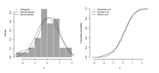
Using the par parameter, it is possible to divide the graphic window in subparts and plot different graphs in it.
> par(mfrow = c(1, 2))
or equivalently,
> op <- par(mfrow=c(1,2))
gives one graph on the left and one graph on the right (the graphical window is divided in two, symmetrically): c(1, 2) means one row and two columns. By saving the current parameters, one can restore the previous parameters using par(op). The hist function is used to compute and plot the histogram of the sample. With option probability=TRUE, the axis is not a count of observations with a partition, but the density, so that the histogram has a total area of 1.
> hist(X,xlab="X",ylab="Density",main="",col="grey",
+ border="white",probability=TRUE)
It is possible to add lines and curves on the graph, for instance the density of a normal distribution fitted using moment estimators,
> u <- seq(min(X)-1,max(X)+1,by=.01)
> lines(u,dnorm(u,mean(X),sd(X)),lty=2)
or a kernel-based estimator of the density, with a Gaussian kernel (this option can be changed through kernel), and the standard rule-of-thumb for choosing the bandwidth from Silverman (1986),
> d <- density(X)
> lines(d$x,d$y)
Actually, because the output of the density() function contains two vectors named x and y, it is possible to use instead
> lines(density(X))
Finally, we can add a legend in the upper left corner (using the "topleft" option, but it might be located anywhere):
> legend("topleft",c("Histogram","Normal density","Kernel density"),
+ col=c("grey","black","black"),lwd=c(NA,1,1),lty=c(NA,2,1),
+ pch=c(15,NA,NA),bty="n")
Note that to locate an area of the graph which might be appropriate for the legend (the text can be placed interactively via a mouseclick), it is possible to use
> legend(locator(1), ...)
Next we plot the empirical cumulative distribution function, computed using
> F.empirical <- function(y) mean(X<=y)
Then we plot it using the standard plot function. Note that to plot a step-function, we use a type="s" style
> plot(u,Vectorize(F.empirical)(u),type="s",lwd=2,col="grey",
+ xlab="X",ylab="Cumulative probability",main="",axes=FALSE)
So far, with the axes=FALSE option, there are no axes on the graph. We can add the x-axis below and the y-axis on the left using
> axis(1); axis(2)
Then, we can add two lines, the distribution function obtained by cumulating the kernel density estimator, and the distribution function of a Gaussian random variable where µ is the empirical mean and σ the empirical standard deviation,
> lines(d$x,cumsum(d$y)*diff(d$x)[1])
> lines(u,pnorm(u,mean(X),sd(X)),lty=2)
Again, in the upper left corner, we can add a legend,
> legend("topleft",c("Empirical c.d.f.","Normal c.d.f.","Kernel c.d.f"),
+ col=c("grey","black","black"),lwd=c(2,1,1),lty=c(1,2,1),bty="n")
If we do not know where to plot the legend, it is possible to use the locator function,
> legend(locator(1),c("Empirical c.d.f.","Normal c.d.f.","Kernel c.d.f"),
+ col=c("grey","black","black"),lwd=c(2,1,1),lty=c(1,2,1),bty="n")
In that case, R reads the position of the graphics cursor when the mouse button is pressed.
Note that graphs are displayed in the graphics window of R. It is possible to export them in a standard image format (bmp, jpeg, png and also pdf). One should add
> png(filename = "rplot.png", width = 480, height = 240,
+ units = "px", bg = "white")
before the plot command (several options can be included), and then add
> dev.off()
at the end (indicating that we are done creating the plot). An alternative, if we want to save a graph that has been plotted, without running again the code, is to use save the output of the graphic window in the .eps format by right-clicking the mouse (or any other format, see Murrell & Ripley (2006) for more details).
1.3.7.3 Graphs That Can Be Obtained from Standard Functions
It is possible to use graphical functions in R that extract information from complex objects such as the ones obtained from a regression model:
> data(StormMax)
> StormMaxBasin <- subset(StormMax,(Region=="Basin")&(Yr>1977))
> attach(StormMaxBasin)
Note here the use of function subset(). Indeed, to keep only some variables in a dataset; one can use the following generic code
> df <- subset(df, select = c(X1,X2))
or, to drop some variables,
> df <- subset(df, select = -c(X1,X2))
The first graph, on the left of Figure 1.4, contains boxplots, per year. We can use boxplot(Wmax~as.factor(Yr)) to display several boxplots on the same graph (vertically here):
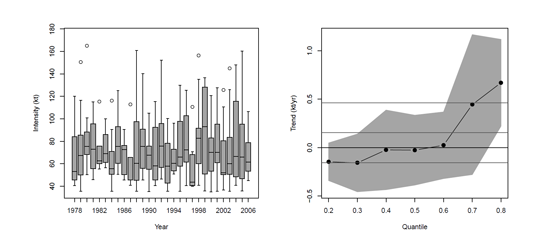
Boxplots of cyclone intensity (kt), per year, and slope of quantile regressions (intensity versus years), for different probability levels.
> boxplot(Wmax~as.factor(Yr),ylim=c(35,175),xlab="Year",
+ ylab="Intensity (kt)",col="grey")
> library(quantreg)
> model <- rq(Wmax~Yr,tau=seq(0.2,0.8,0.1))
> model
Call:
rq(formula = Wmax ~ Yr, tau = seq(0.2, 0.8, 0.1))
Coefficients:
tau= 0.2 tau= 0.3 tau= 0.4 tau= 0.5
(Intercept) 189.8900242 391.2367884 140.80069596 210.10132020
Yr -0.0715789 -0.1696345 -0.04040035 -0.07219432
tau= 0.6 tau= 0.7 tau= 0.8
(Intercept) 7.500000e+01 -221.78568 -1169.6654437
Yr -1.075529e-16 0.15365 0.6361049
Here, seven regressions have been computed and stored in the model object. Using the summary() function on this object, many interesting quantities can be computed (for example, confidence intervals on parameters) and then plotted. The following graph is on the right of Figure 1.4.
> plot(summary(model,alpha=0.05,se="iid"),
+ parm=2,pch=19,cex=1.2,mar=c(5,5,4,2)+0.1,
+ ylab="Trend (kt/yr)",xlab="Quantile")
1.3.7.4 Adding Shaded Area to a Graph
Consider the case where we want to sketch the possible range for a quantile function. Assume that X and Y are two N (0, 1) random variables, and let us plot the upper and the lower bound for the quantile function of X + Y . If Finv (that is, F −1) denotes the quantile function of X , and Ginv (that is, G−1) the quantile function of Y , then those bounds can be computed using (see Williamson (1989) for theoretical details, as well as algorithms):
> n <- 1000
> Qinf <- Qsup <- rep(NA,n-1)
> for(i in 1:(n-1)){
+ J <- 0:i; Qinf[i] <- max(Finv(J/n)+Ginv((i-J)/n))
+ J <- (i-1):(n-1); Qsup[i] <- min(Finv((J+1)/n)+Ginv((i-1-J+n)/n))
+}
Then, lines are drawn using the lines function, for example,
> x <- seq(1/n,1-1/n,by=1/n)
> lines(x,Qsup,lwd=2)
and to add colored area, we use the polygon function. The color is chosen within the gray palette,
> gray.col <- gray.colors(n=100, start = 0, end = 1)
from library(RColorBrewer). To colorize between the upper bound Qsup and the sum of quantile functions, qnorm(.,sd=2), the code is
> polygon(c(x,rev(x)),c(Qsup,rev(qnorm(x,sd=2))),col=gray.col[45],border=NA)
It is also possible to look at constraint bounds, when we assume that X and Y are positively dependent (with quadrant positive dependence, i.e. for all x, y, ℙ(X > x, Y > y) ≥ ℙ(X > x) · ℙ(Y > y), or equivalently ℙ(X > x|Y > y) ≥ ℙ(X > x)) In that case, those bounds can be computed using
> Qinfind <- Qsupind <- rep(NA,n-1)
> for(i in 1:(n-1)){
+ J <- 1:(i); Qinfind[i] <- max(Finv(J/n)+Ginv((i-J)/n/(1-J/n)))
+ J <- (i):(n-1); Qsupind[i] <- min(Finv(J/n)+Ginv(i/J))
+}
Then, we use
> polygon(c(x,rev(x)),c(y.lower,rev(y.upper)),col=gray.col[45],density=20,border=NA)
where y.upper and y.lower are the upper and the lower curves for the area that should be colorized.
1.3.7.5 3D Graphs
Finally, note that 3D graphs can also easily be constructed. Use here
> x <- y <- seq(-2.5,2.5,by=.25)
> z <- outer(x,y,function(u,v) binorm(u,v,r=.4))
To visualize level curves, use
> image(x,y,z,col=rev(gray.col))
> contour(x,y,z,add=TRUE)
Here, contour lines are added to the colorized graph. For surfaces of densities, use
> persp(x,y,z)
Because we keep visualizing graphs on a screen, a 3D graph is just a 2D visualization. It is possible to define an object, storing the transformation matrix used for that representation
> pmat <- persp(x,y,z,theta=210, col=gray.col[45],shade=TRUE)
> pmat
[,1] [,2] [,3] [,4]
[1,] -3.464102e-01 0.05176381 -0.1931852 0.1931852
[2,] -2.000000e-01 -0.08965755 0.3346065 -0.3346065
[3,] 3.526252e-16 11.12516046 2.9809778 -2.9809778
[4,] -3.061800e-17 -0.96598365 -2.9908853 3.9908853
We can still use 2D graphical functions to add lines or points on the figure. For instance, to draw a line, that is, (xt , yy , zt)t∈ [a,b] , use function trans3d(),
> u <- x; v <- rep(1,length(y)); w <- binorm(u,v,r=.4)
> lines(tranS3d(u,v,w, pmat),lwd=4,col="black")
1.3.7.6 More Complex Graphs
In many applications, we might like to enhance plots, in order to visualize various interesting features in one single graph. In previous sections we have seen how to plot several curves (and lines) on the same graph. With the following code we can plot two different regression lines, for two different factors (here Z takes values M or F), the output being the graph on the left of Figure 1.7,
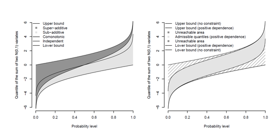
Admissible values for the quantile function of the sum of two N (0, 1) random variables, with, on the right, the restriction when X and Y are positively dependent.


Regression lines of Y against X , for different values of a factor Z , with trellis functions on the right.
> attach(linearmodelfactor)
> plot(X,Y,pch=(Z=="M")*2+1)
> abline(lm(Y~X,data=B,subset=which(B$Z=="M")))
> abline(lm(Y~X,data=B,subset=which(B$Z=="F")),lty=2)
> legend("topright",c("M","F"),pch=c(3,1),lty=c(1,2),bty="n")
Another way of visualizing those regression lines is by trellis-type graphics (as introduced in Cleveland (1993)) using the lattice library (see also Sarkar (2002)).
> xyplot(Y ~ X| Z, panel = function(x, y) {panel.xyplot(x, y);panel.lmline(x, y)})
In the first part, we ask for graphs for different values of Z, of Y against X. In the second part, we specify a generic function that will be added to the scatterplot (here, a linear regression line). Those two graphs are on the right of Figure 1.7. Observe that—automatically—the same y-axis is used, to allow for comparisons. More details on trellis graphs can be found in Sarkar (2008).
With standard functions, it is also possible to plot two or more figures on a single graph. Graphics parameters mfrow and mfcol subdivide the plotting region into arrays of figure regions, as discussed previously. But graphics will have the same size. It is possible to have Windows of different shapes on a single graph using either mai or mar in the par description (margin sizes are either in inches with mai, or in text line units with mar).
Consider the case where we wish to plot surfaces and contour plots (with level curves) to visualize dependencies, as well as histograms to describe marginal distributions. Consider for instance the popular loss-ALAE dataset (see e.g. Klugman & Parsa (1999)), with indemnity payment (loss), and the allocated loss adjustment expense (ALAE), for 1,500 individual claims, in U.S. dollars:
> library(evd); data(lossalae); library(MASS)
> X <- lossalae[,1]; Y <- lossalae[,2]
> xhist <- hist(log(X), plot=FALSE)
> yhist <- hist(log(Y), plot=FALSE)
> top <- max(c(xhist$counts, yhist$counts))
In order to visualize the distribution of the points, consider the bivariate kernel estimator of the joint density of (X, Y):
> kernel <- kde2d(log(X),log(Y),n=201)
Those histograms (in the xhist and yhist object) and surfaces (in the kernel object)
can be plotted on the same graph using the following code:
> par(mar=c(3,3,1,1))
> layout(matrix(c(2,0,1,3),2,2,byrow=TRUE),
> c(3,1), c(1,3), TRUE)
The window will be split into four parts, ![]() , in that specific order, and if the length of the last column and the first row is 1, the length of the first column and the last row will be 3.
, in that specific order, and if the length of the last column and the first row is 1, the length of the first column and the last row will be 3.
> plot(X,Y, xlab="", ylab="",log="xy",col="grey25")
> contour(exp(kernel$x),exp(kernel$y),kernel$z,add=TRUE)
> par(mar=c(0,3,1,1))
> barplot(xhist$counts, axes=FALSE, ylim=c(0, top),space=0,col="grey")
> par(mar=c(3,0,1,1))
> barplot(yhist$counts, axes=FALSE, xlim=c(0, top),space=0,
+ horiz=TRUE,col="grey")
This graph is on the left of Figure 1.8. Color grey25 has been used to get a wider palette of colors. But other functions can be used, for instanced gray.colors() (from the grDevices package) can be used to generate a palette:
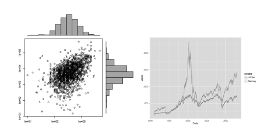
Scatterplot of the loss and allocated expenses dataset, including histograms, on the left, with a graph obtained using the ggplot2 library.
> gray.colors(8)
[1] "#4D4D4D" "#737373" "#8E8E8E" "#A4A4A4"
[5] "#B7B7B7" "#C8C8C8" "#D7D7D7" "#E6E6E6"
For other palettes, one can use library RColorBrewer, :
> brewer.pal(n=8, "Greys")
[1] "#FFFFFF" "#F0F0F0" "#D9D9D9" "#BDBDBD"
[5] "#969696" "#737373" "#525252" "#252525"
Use display.brewer.all() to visualize a lot of possible palettes.
Finally, to get elegant graphs, an alternative can be to use the ggplot2 library, where the first two letters stand for grammar of graphics; from Wilkinson (1999) and Wickham (2009). This library is based on the reshape and plyr packages. The idea is to use different layers to generate a complex graph. For instance, consider two financial indices:
> library(tseries)
> SP500 <- get.hist.quote("^GSPC")
> Nasdaq <- get.hist.quote("^NDX")
> BS <- data.frame(Date=time(SP500),SP500=SP500$Close)
> BSN <- data.frame(Date=time(Nasdaq),Nasdaq=Nasdaq$Close)
> B <- merge(BS,BSN)
> indices <- melt(B, id.vars = "Date")
The graph is on the right of Figure 1.8. More details on ggplot2 graphs can be found in Wickham (2009).
Note here the use of the merge() function. This function merges two dataframes by common columns (or row) names. This function can perform one-to-one, many-to-one and many-to-many merges. If we want to plot the two series, the code is close to the one used in the lattice package:
> zp1 <- ggplot(indices)
> zp1 <- zp1 + geom_line(aes(x = Date, y = value, colour = variable))
> plot(zp1)
1.4 More Advanced R
As mentioned earlier, the aim of this chapter is to introduce basics about the R language. Of course, it is possible to optimize the code. But it is clearly a matter of personal taste, and priorities. It might be important to have codes that will make a procedure run faster, but it might also be important to have readable codes, or to have codes that run on a desktop or a laptop, not necessarily a server.
So far, we have seen a lot of things that R can do. But R has limitations too. R is a bit slow in some computations (as discussed earlier), and sometimes R cannot define objects that are too large. In this section, we will briefly show how to code advanced functions in R.
1.4.1 Memory Issues
The memory R can use depends on several factors:
- The RAM physically in the computer
- The RAM used by the computer (by other programs)
- The processor (32 or 64 bits) as the allocated RAM is bounded at 232 bytes (i.e. 4 × 1024 KB, or 4 GB) for 32 bits, while it might be 264 bytes for 64 bits (but in that case, the limit comes from the architecture of the processor)
Recall that to get numerical characteristics of the computer, one should use the .Machine object. For instance,
> .Machine$sizeof.pointer
[1] 4
returns 8 on 64-bit builds, and 4 for 32-bit. On a 32-bit computer, some operations are not possible; for instance,
> D<-matrix(0,12000,12000)
Error: cannot allocate vector of size 1.1 GB
but
> D <- matrix(0,10000,10000)
does work
> object.size(D)
800000112 bytes
If the dataset is a very large one, we might not have enough memory to run standard regression functions. Some functions (slower than the standard regression functions) will work when there is not enough memory to use the standard functions. Namely,
> library(biglm)
> fit <- biglm(Y ~ X1 + X2, data=base)
1.4.2 Parallel R
It is possible to do calculations faster using several processors, all of them cooperating on a given task. The idea of parallel processing is to break up the task, to split it among multiple processors, and then to put the components back together. This is very useful and easy if the task can be split up (especially without any communication between them, like using a value computed on one processor on another one, as discussed in Yu (2002) or more recently Schmidberger et al. (2009) and Hoffmann (2011)). In the plyr package, it is possible to use option .parallel=TRUE in the aaply() function, for instance. It is also possible to use libraries dedicated to parallelization; see Schmidberger et al. (2009) for a description of the state of the art. The following code was run on a 4 core computer:
> library(parallel)
> (allcores <- detectCores(all.tests=TRUE))
[1] 4
With the snow package, tasks are sent to the processors (that can also be clients on a complex server), then results are sent back and assembled into the final output. One can also use package doMC:
> library(doMC)
> registerDoMc()
where register determines the number of cores to use. Consider here the following function, where a loop is used and at each iteration, outputs are stored in a list:
> F<-function(n,m=100){
+ L<-vector("list", n)
+ for(i in 1:n)
+ {
+ X<-rnorm(m,0,sd=log(1+i))
+ L[[i]]<-max(eigen(X%*%t(X))$values)
+ }
+ return(L)
+}
It is possible to make the algorithm faster using a parallelized foreach %dopar% loop, that always returns a list:
> parF<-function(n,m=100){
+ foreach(i = 1:n) %dopar%
+ {
+ X<-rnorm(m,0,sd=log(1+i))
+ L[[i]]<-max(eigen(X%*%t(X))$values)
+ }
+}
Here, the parallelized function is slightly faster on a desktop:
> microbenchmark(F(), parF(), times = 10) Unit: milliseconds
expr min lq median uq max
1 F() 285.3781 288.3071 290.9585 306.8264 340.7759
2 parF() 218.4247 224.5321 226.0498 237.5514 255.7262
Remark 1.1 Random number generation might be a good example of tasks that can be split among multiple processors, but one should keep in mind that random number generators are iterative, and thus theoretically not splittable.
The idea is that if we work on a typical desktop, then implementing parallel processing in some R code might speed up your program. But not every task runs better in parallel. Further, distributing processes among the cores may cause computation overhead: we might lose time (and memory) firstly by distributing, secondly by gathering the patches shared out among the processing units. So, sometimes parallel computing can be rather inefficient. Consider the case where we generate datasets with a possibly large number of rows, and we have to compute, say, quantiles per column. To compare the use of (standard) lapply() with mclappy() from library multicore, parLapply() from library snow or sfLapply() of library snowfall, we generate a dataframe with 100 columns and n =250,000 rows.
> n <- 250000
> base <- data.frame(matrix(rnorm(n*100),n,100))
The goal can be to compute quantiles per column. Consider here the following function:
> microbenchmark(
+ mclapp=data.frame(mclapply(base, quantile, probs = 1:3/4 ,
+ mc.cores = allcores)),
+ mlapp=data.frame(lapply(base, quantile, probs = 1:3/4)),
+ sflapp=data.frame(sfLapply(base, quantile, probs = 1:3/4)),
+ times=100)
Unit: milliseconds
expr min lq median uq max
1 mclapp 710 744 785 811 951
2 mlapp 1444 1465 1524 1562 1788
3 sflapp 1443 1470 1530 1567 1787
In this example, mclapp() is (only) twice as fast as simply lapply(). Even with 250,000 rows, parallel codes on a small number of cores are not very efficient.
Remark 1.2 In order to go even faster, it is also possible to run computations not on the CPU (central processing unit), but on the GPU (graphical processing unit), using the gputools on a Linux system. But in the sequel, we will simply dispatch each task to a different CPU core.
1.4.3 Interfacing R and C/C++
As mentioned earlier, R code is interpreted when it is run, unlike some other languages that are first compiled. But R actually does have compiling abilities that might speed up functions by a factor of 3 or 4. A first strategy is to use .Internal, which may speed up some functions but is only recommended for R-wizards:
> u <- runif(100)
> benchmark(mean(u),sum(u)/length(u),.Internal(mean(u)),replications=1e5)[,c(1,3,4)]
test elapsed relative
3 .Internal(mean(u)) 0.320 1.000
1 mean(u) 0.870 2.719
2 sum(u)/length(u) 0.339 1.059
Another strategy is to use the compiler library. Consider the case where we want to compute the sum per row, of a given matrix:
> library(compiler)
> f1 <- function(x) apply(x,1,sum)
> g1 <- cmpfun(f1)
Note that it might be more efficient to use a loop, instead of using a R function:
> f2 <- function(x) {
+ v <- rep(NA,nrow(x))
+ for(i in 1:length(v)) v[i] <- sum(x[i,])
+ return(v)}
> g2 <- cmpfun(f2)
We can now compare those four functions:
> n <- 100
> M <- matrix(runif(n^2),n,n)
> benchmark(f1(M),f2(M),g1(M),g2(M),
+ replications=1000)[,c(1,3,4)]
test elapsed relative
1 f1(M) 0.519 1.736
2 f2(M) 0.462 1.545
3 g1(M) 0.485 1.622
4 g2(M) 0.299 1.000
Observe that the compiled function of the second code, obtained using cmpfun, is almost twice as fast as the apply() function here. One could also have used rowSums() or the even faster internal function .rowSums.
Finally, if R is not fast enough, to improve performance, it is possible to write key functions in C/C++, by ourselves. Use of C/C++is more appealing than Fortran, for instance, because of the Rcpp API (application programming interface), as discussed in Lang (2001). Note that to use the Rcpp package on a Windows platform, it is necessary to install (properly) the Rtools kit (but this is straightforward on Mac or Linux).
> library(Rcpp)
> evalCpp("7+3")
[1] 10
It is possible to create ad-hoc R functions, such as a function square() that will compute the square of any integer:
> cppFunction("int square(int x) {return x*x;}")
> square(9)
[1] 81
or power() that will compute; more generally; the power n of any (positive) number x:
> cppFunction("double power(double x, int n){double xn = pow(x,n);return xn;}")
> power(4,2)
[1] 16
Following Eddelbuettel & Fran¸cois (2011), consider the construction of the Fibonacci sequence, define recursively by
The R code to define that function is
> FibonacciR <- function(n){
+ if(n<2) return(n)
+ else return(FibonacciR(n-1)+FibonacciR(n-2))
+}
> FibonacciR(10)
[1] 55
(see the previous example of the towers of Hanoi for recursive programming) but it can be very slow to run (even for a small n),
> system.time(FibonacciR(35))
user system elapsed
35.431 0.128 35.538
The C/C++code to compute that sequence is
int g(int n) {if(n<2) return(n) ; return(g(n-1)+g(n-2));}
It is possible to use that function in the following R code:
> library(Rcpp)
> cppFunction("
+ int FibonacciC(int n){
+ if (n<2) return(n) ;
+ else return(FibonacciC(n-1)+FibonacciC(n-2));
+}")
The output is hopefully, the same as the R function:
> FibonacciC(10)
[1] 55
but here, the code is much faster to run (here, 1,000 times faster):
> library(rbenchmark)
> benchmark(FibonacciR(30),FibonacciC(30),replications=1)[,c(1,3,4)]
test elapsed relative
2 FibonacciC(30) 0.004 1
1 FibonacciR(30) 4.136 1034
It is possible to use a standard R function to compute vectorized versions of that function. Using Vectorize() or sapply() yields comparable computation times. But again, using C/C++ will make our code run 1,000 times faster!
> N=1:35
> benchmark(sapply(N,FibonacciR),Vectorize(FibonacciR)(N),
+ sapply(N,FibonacciC),Vectorize(FibonacciC)(N),replications=1)[,c(1,3,4)]
test elapsed relative
3 sapply(N, FibonacciC) 0.094 1.000
1 sapply(N, FibonacciR) 91.888 977.532
4 Vectorize(FibonacciC)(N) 0.099 1.053
2 Vectorize(FibonacciR)(N) 91.566 974.106
For further information about the C/C++ language, see Kernighan (1988) or Stroustrup (2013).
It is also possible to use more complex formats than integers (int) or reals (double). For instance, from a matrix, it is possible to return a vector,
> cppFunction("
+NumericVector SumRow(NumericMatrix M) {
+ int nrow = M.nrow(), ncol = M.ncol();
+ NumericVector out(nrow);
+ for (int i = 0; i < nrow; i++) {
+ double total = 0;
+ for (int j = 0; j < ncol; j++) {
+ total += M(i, j);
+}
+ out[i] = total;
+ }
+ return out;
+}
+ ")
> SumRow(matrix(1:6,3,2))
[1] 5 7 9
which returns the sum per row.
For those not familiar with C/C++, using package RPy, it is also possible to call R using Python.
1.4.4 Integrating R in Excel®
Though actuaries might be interested in advanced methods to run smoothing techniques on large datasets (that will be memory—and time—consuming), in practice they also like to use Excel and Visual Basic for simple reporting. An interesting feature of R, mentioned in Baier & Neuwirth (2003), is that “R can completely control any of the Office applications—at least as far as Office allows this”.
To import data from Excel spreadsheets, run computations in R and then export R outputs in Excel spreadsheets; it is possible to use the XLConnect package,.
> library(XLConnect)
> writeWorksheetToFile(file=’test.xlsx’,data=M,sheet=’test’,
+ startRow = 10, startCol = 3)
for some matrix M.
An alternative is to use the following nice tool, described in Courant & Hilbert (2009): the Excel add-in RExcel.xla that allows one to use R from within Excel® , using the library(rcom). R can be used in a scratchpad mode that consists of writing R code directly in an Excel worksheet and transferring scalar, vector, and matrix variables between R and Excel. But R can also be called directly in functions in worksheet cells. An alternative is to use a macro mode where the user can write macros using Visual Basic and R codes. For instance, within a cell of a worksheet, one can compute the value of an R function rfunction (with one parameter) by typing =RApply(’rfunction’,A1) in a cell, assuming the parameter is the value given in cell A1.
1.4.5 Going Further
The most difficult task for R users is probably to follow the active community of R users. Academic publishers now have their own R collections, with ‘The R Series’ of Chapman & Hall/CRC, and the ‘UseR!’ of Springer Verlag. There are several books on the R language, such as Cohen & Cohen (2008), Dalgaard (2009), Krause (2009), Zuur et al. (2009), Teetor (2011), Kabacoff (2011), Maindonald & Braun (2007), Craley (2012), or Gandrud (2013), to mention only some of them. On top of those general books, one can easily find books dedicated to specific topics, such as Wickham (2009), Murell (2012), Lawrence & Verzani (2012), Højsgaard et al. (2012) on graphics (mainly, not to say only). Hundreds of books related to S and R are mentioned at http://www.r-project.org/doc/bib/R-books.html, including books that are related to S or R. Free ebooks can be found at http://cran.r-project.org/manuals.html or http://cran.r-project.org/other-docs.html.
It is also possible to follow updates through the R Journal, available online at http://journal.r-project.org/. This journal contains short introductions to R packages, and hints for newcomers as well as more advanced programmers. The journal contains updates about R conferences, and R user groups, that can be found now in almost any (large) city. R bloggers also provide examples, codes, and hints that can be useful to anyone willing to learn more about R.
1.5 Ending an R Session
This introduction was a bit long. And it might be time to close R. One way to exit (properly) R is to use the q() function:
> q()
R will then ask whether to save the workspace image, or not.
Save workspace image? [y/n/c]:
Answering n (for ‘no’) will exit R without saving anything, whereas answering y (for ‘yes’) will save all defined objects in a file .RData, and the command history will be stored in a file called .Rhistory, both in the working directory. Note that those two files are text files and can be opened using any text editor.
1.6 Exercises
- 1.1. What is the difference between a data.frame and a data.table object?
- 1.2. What is the difference between read.table() and read.ftable() functions?
- 1.3. Display the value of log(4) with fifteen digits.
- 1.4. What is function intersect for? What would intersect(seq(4,28,by=7), seq(3,31,by=2)) return?
- 1.5. What would c(TRUE, TRUE, FALSE, FALSE) & c(TRUE, FALSE, FALSE, TRUE) return?
- 1.6. Import file extremedatasince1899.csv with years from 1900 to 2000 only.
- 1.7. Sort the previous variable according to variable Wmax.
- 1.8. From database extremedatasince1899.csv, compute the average value of variable Wmax when Region is equal to Basin.
- 1.9. Using the xtable package, generate an html page that contains a table, obtained from the sub-dataset of extremedatasince1899.csv where Region is equal to Basin, and Yr is between 1950 and 1959.
- 1.10. Still from the same file, create a sub-dataset that contains only variables that are numeric.
- 1.11. What is function attach used for?
- 1.12. What will the following lines return?
> n<<--1> if (n==0) "yes" else "no"; n> if (n < - 0) "yes" else "no"; n> if (n<-0) "yes" else "no"; n> if (n=0) "yes" else "no"; n> if (n<-2) "yes" else "no"; n1.13. Explain the results of the statements below:
> 9*3 ^-2; (9*3)^-2> -2^-.5; (-2)^-.5> 1:4^2; 1:4*4> 2^2^3; 2-2-3> n <- 5; for (i in 1 : n+1) print(i)> k <- 1:3; k[3]^2; k^2; k^2[3]1.14. Are the results of the following statements as you expected?
> c(1, 7, NA, 3) == NA; is.na(c(1, 7, NA, 3))> Inf*Inf; 0*Inf; Inf*-Inf; Inf>Inf/2; sqrt(Inf)> 2^1023.999<Inf; 2^1024<Inf> 1/0; 0/0> log(0); log(-1)> sqrt(-1); sqrt(-1+0i)> integrate(dnorm, 0, 20)> integrate(dnorm, 0, +Inf)> integrate(dnorm, 0, 20000) - 1.15. What will 1:10*1:5 return?
- 1.16. Given a vector x, write a function which returns only elements of x larger than mean(x).
- 1.17. Write a function seqrep(n) which returns vector (1, 2, 2, 3, 3, 3, . . . , n) where integer k is repeated k times. How long is this vector when n = 50?
- 1.18. Write a function that counts the number of NA’s in a vector.
- 1.19. Create a function second.diag(M) which returns the second diagonal of squared matrix M.
- 1.20. What will M[,2] return if M <- matrix(1:5,3,3)?
- 1.21. Get the help page on command %%. What does that mean for x if x %% 3 == 0 is TRUE?
- 1.22. Given matrix m <- matrix(1:20,5,4), what will which(m %% 3 == 0, arr.ind=TRUE) produce?
- 1.23. Write a function that computes the power of any square matrix, power(M,n).
- 1.24. Which function should you use to compute M −1 ?
- 1.25. Create the identity matrix of size 5 × 5.
- 1.26. Write a function to compute sin2 (x) + x/10. Find its minimum in (0, 2π).
- 1.27. Using commands ! and %in%, return the subvector x <- sample(1:15) where values c(3,7,12) are removed.
- 1.28. Given a matrix M , write a function which returns the following Kronecker product:
- 1.29. Compute
- 1.30. Solve numerically the following system
- 1.31. Given a vector x in ℝn and a function f : ℝ → ℝ, create a function sum.function(x,f) which computes
- 1.32. Compute
- 1.33. Create a function mat(n) which returns the n × n matrix, such that and 0 elsewhere.
- 1.34. Are sqrt(7) and 7^.5 equal?
- 1.35. Given a <- c(-0.2,0.2,0.49,0.5,0.51,.99,1.2), what is the difference between trunc(a), floor(a), ceiling(a) and round(a)?
- 1.36. Given a vector x, use function ifelse() to generate a vector with the same length as x with the logarithm of elements of x that are positive, and NA when elements are negative.
- 1.37. Create a function anagram(word1,word2) which returns TRUE if word1 and word2 are anagrams.
- 1.38. Find roots of polynomial .
- 1.39. What is function pretty used for?
- 1.40. Given a vector x, write a function which.closest(x,x0) which returns the element in x that is the closest to x0.
- 1.41. Given two vectors x and y, write a function subcount(y,x,k) which returns the number of elements of y smaller than x[k].
- 1.42. Create vector of length 100 ’Ins1’,’Ins2’, . . . , ’Ins100’.
- 1.43. Create vector c("London (2012)","Beijing (2008)","Athens (2004)", "Sydney (2000)") from c("London","Beijing","Athens","Sydney").
- 1.44. What will the two functions return, paste("a", c("b c","d"), sep="") and paste("a", c("b c","d"), collapse="")?
- 1.45. What will grep("ab",c("abc","b","a","ba","cab")) return?
- 1.46. What is function apropos() used for?
- 1.47. Given a vector x, what function(s) can be used to return the location of the largest element?
- 1.48. Define Z <- ts(rnorm(240), start=c(1960,3), frequency=12). Compute the sum of elements of time series Z related to January.
- 1.49. Create a matrix with four columns, that contains all combination of four terms in c(1,2,7,6,12,37,59), each row being a combination.
- 1.50. Get the help page on command %o%.
- 1.51. What will the following lines return?
> as.integerc(TRUE,FALSE))> (-2:2)==TRUE> (-2:2)==FALSE> as.logical(-2:2) - 1.52. Generate a vector x <- rpois(7,4). What does unique(sort(x))[1:3] return? What about sort(unique(x))[1:3]?
- 1.53. In function density(), what is parameter n used for?
- 1.54. Given a matrix M, write a function range.row which returns a vector whose ith entry is the difference between the largest and the smallest value on the ith row of M.
- 1.55. Find the dataset accident from package hmmm. How many rows does the dataset have?
- 1.56. On dataset accident, what is the average of variable Freq if the dataset is restricted to Type equal to uncertain?
- 1.57. What is function save.image() for?
- 1.58. Write a qqplotQ(x,q) function which plots the standard QQ plot function, for a sample x, and a quantile function q().
- 1.59. Given a vector x and a cumulative distribution function F, write a function which plots the associated PP-plot.
- 1.60. Compute the integral of f (x) = x · log(x) on [0, 1].
- 1.61. Plot x ↦ f(t)dt, where f (x) = x · log(x), on [0, 1].
- 1.62. What is the minimum of function f on [0, 1]?
- 1.63. When plotting y against x using plot(), what will option asp=1 do?
- 1.64. When plotting y against x using plot(), what will options xaxs="i" and yaxs="i" do?
- 1.65. When plotting y against x using plot(), what will option las=3 do?
- 1.66. When plotting y against x using plot(), what will option xlim=rev(range(x)) do?
- 1.67. Before a plot() call, what happens if we add par(bg = "thistle")? How do we restore the initial parameters?
- 1.68. To save a graph in pdf format, one can use function dev.print(). How should it be used?
- 1.69. What is the quantile of the N (0, 1) distribution, for probability 95%?
- 1.70. Using Monte Carlo simulations, approximate E[cos(X)], where X ~ N (0, 1).
- 1.71. Using Monte Carlo simulations, approximate the density of max{Bs , s ∈ [0, 1]}, where (Bs) is a standard Brownian motion.
- 1.72. Plot the quantile function of the N (0, 1) distribution, on [1%, 99%]. With a red line.
- 1.73. In function persp(), what is the difference between col="red" and border="red"?
- 1.74. Using several calls of function contour option levels, reproduce the graph in the upper left corner of Figure 1.6 where levels curves are in red when density is lower than 0.1, and in blue when density is over 0.1.
- 1.75. What will Df <-D(expression(cos(x)/sin(x)), "x") return? If we execute command x <- pi/4, what will eval(Df) return?
- 1.76. Find a package that can help you compute the kurtosis from a vector.
- 1.77. What is the following function testing, for some integer n, function(n) sum(n%%(1:n)==0)==2?
- 1.78. What is Rprof() used for?
1 Note that this function will return numbers slightly different from the ones obtained using prod(1:x) for large values of x. In that case, one might use library(gmp) and either factorialZ(x) or prod(as.bigz(1:x)) (which are now identical).