Chapter 5

Teaching Simple Linear One-Layer Neural Networks

5.1 Building Teaching File

This chapter explains how to teach the simplest neural networks. Theoretical knowledge often gained from reading algorithm descriptions is completely different from hands-on practical knowledge gained from designing an activity and seeing the results. Chapter 4 covered research involving the simplest networks. We built a simple linear network and conducted some research to demonstrate how neurons and networks behave. The experiments in this chapter will expand your knowledge of linear networks.

We will explain linear networks and discuss the limitations imposed by their simple structures. For our purposes, linear networks are easier to teach, they perform certain tasks very well, and their results are easy to analyze. Chapter 6 will cover the more complex nonlinear networks.

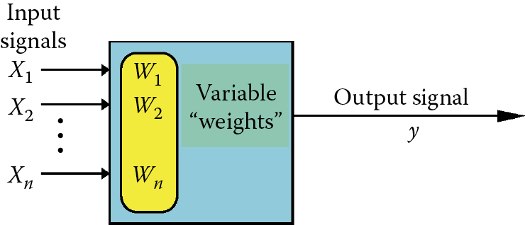
We will start with the easiest of the easy tasks: teaching a single neuron. To achieve this, we will use the Example 03 program that allows us to teach a simple linear neuron (Figure 5.1) and conduct simulation research. However, before we input data and attempt to modify the program, some introductory remarks are appropriate.

During the experiments involving the work of a single neuron serving as an entire network, we input all the needed signals; this gave us full control over the experiment. Working with a larger network performing more difficult tasks is a far different endeavor. Sometimes hundreds or thousands of experiments are needed before a reasonable result appears from the initial chaos. Of course, only a masochist will enter the same data thousands of times to teach a network how to generate a correct task solution.

Therefore, we assume that a teaching process is based on a set of teaching data created by and saved on a computer. The set should include input signals for all the neurons in the network and the models of the correct (required) output signals. The teaching algorithm will use these signals to simulate real network behavior. In our programs, the format of teaching data will be as follows:

• Explanatory comments
• Set of input signals
• Set of models of correct output signals

We assume that the input signals will include five element vectors (including five signals for five inputs of the analyzed neuron) and only one model of the correct output signal because we can temporarily use only one neuron. These network parameters are placed in the first line of the teaching sequence file. A teaching sequence can be as long as you wish. In fact, the more examples with correct solutions you show a network, the better the results. Hence, the file containing all this information may be very large. For a program to teach one neuron, we recommend the use of the following file:

5, 1

A typical object that should be accepted

3, 4, 3, 4, 5

1

A typical object that should be rejected

1, -2, 1, -2, -4

-1

An untypical object that should be accepted

4, 2, 5, 3, 2

0.8

An untypical object that should be rejected

0, -1, 0, -3, -3

-0.8

The above text is a teaching file for Example 03 and may be found in a file called Default teaching set 03.txt. Example 03 will offer you the teaching file at the start. Of course, you can create your own file with data for teaching a network and connect it to the program described below. A teaching file is required to enable your neuron to recognize different sets of target standards or you can train it to build a model to approximate some relationship between input and output signals, for example, resulting from medical observations or physical measurements.

Remember that this neuron is linear and is able to learn only how to transform signals similarly to mathematical methods. As for example, correlation and multidimensional linear regression methods. You will learn about wiser neurons and more common nonlinear networks later. For now, we suggest you use our programs to ensure that your neurons work correctly. Later you can work with your own teaching data tailored to your own tasks.

5.2 Teaching One Neuron

We first load the Example 03 program and try to start it. It loads the data from the Default teaching set 03.txt data and tries to classify objects correctly. Object data are recorded in file in the correct order in the form of input signals for the neuron. A neuron can notice an incorrect operation because the Default teaching set 03.txt file has models of the correct answers recorded by the teacher. The program then modifies the weights of the modeled neuron according to the procedures described in an earlier chapter.

This feature teaches the neuron to perform better when given a defined task. During simulated teaching, the screen will display the progress of the process step by step, show how the weights change, and reveal errors. At the beginning, errors are large, of course, as shown in Figure 5.2.

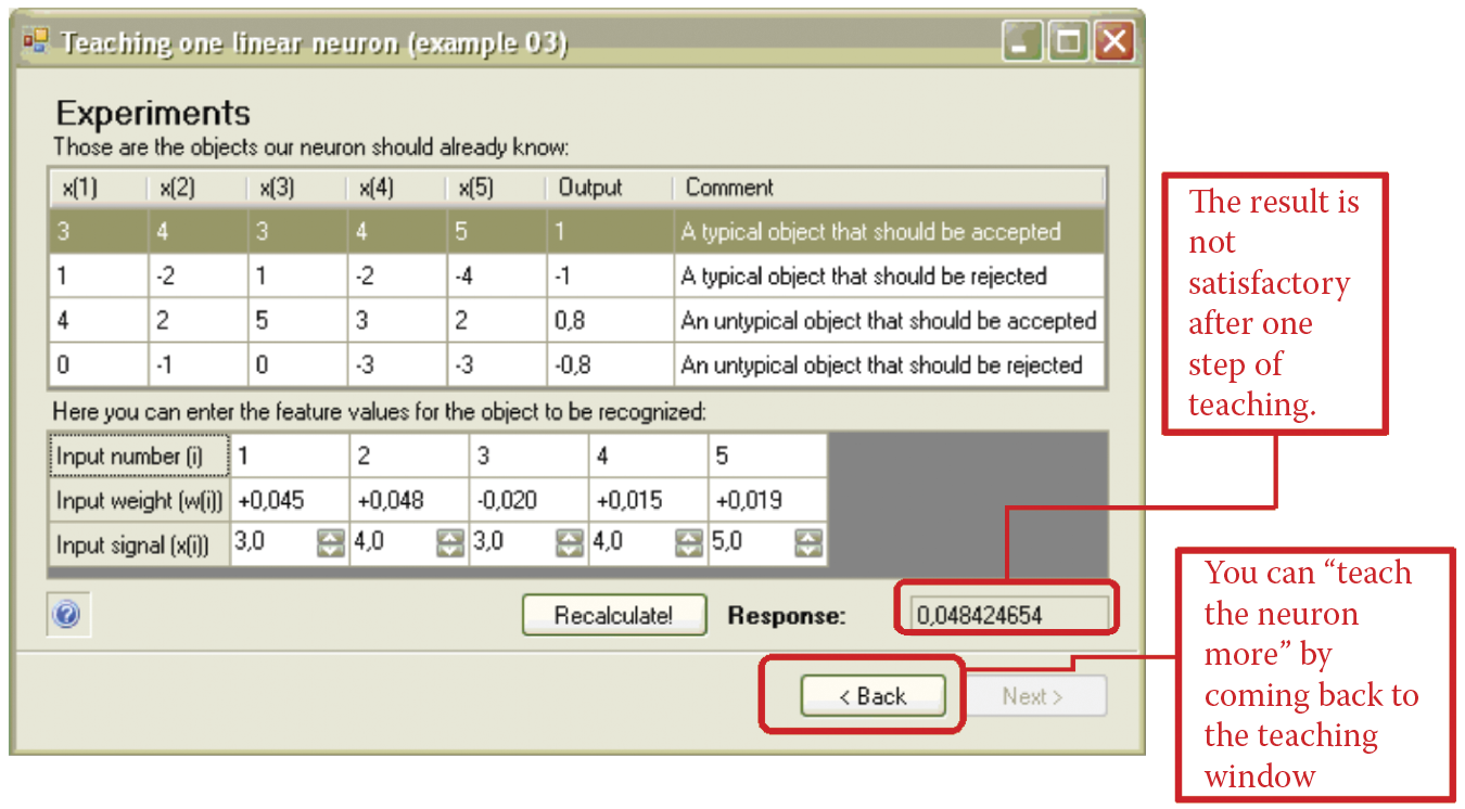
If you are testing the network as you read this (you can go to this phase at any time by clicking Next), you may check its knowledge. However, you will see at the start that the assumption that the neuron should already know the shown objects is incorrect (Figure 5.3).

To allow a neuron to work effectively, it may require more learning. By clicking the Back button, we can return to the previous Teaching window and teach the neuron by clicking the Teach more! button several times. After analyzing errors again, you may find they have not decreased significantly after further teaching (cf. Figure 5.4). You can stop teaching and try to estimate network knowledge by using the example again. The results should be better (Figure 5.5). The results of advanced teaching are shown in Figure 5.6.

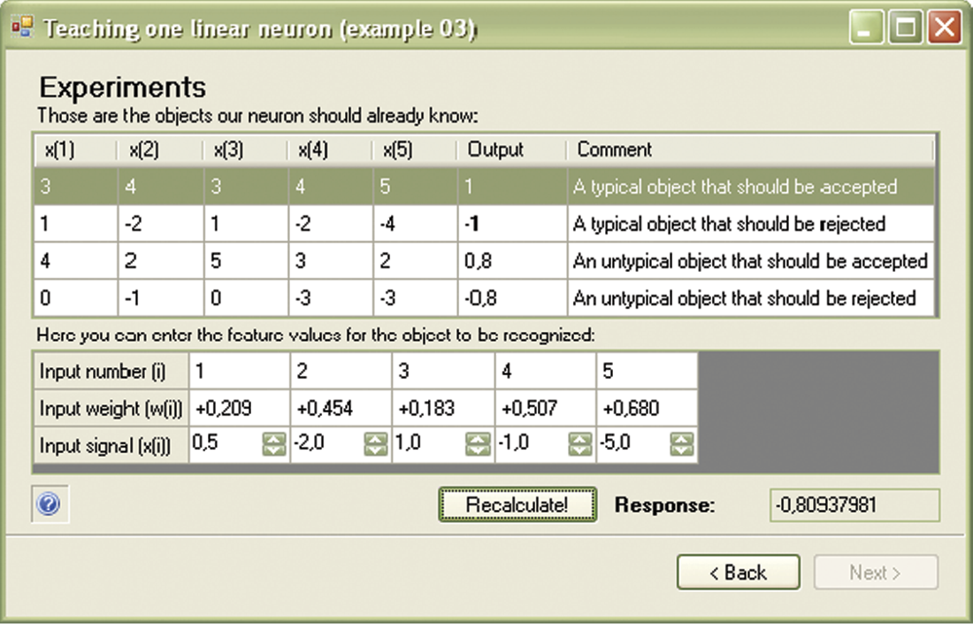
During advanced teaching, the network definitely rejects objects that are only similar to the objects from teaching set and should be rejected as shown in Figure 5.5. During teaching, you can review the history of the process that appears on request in the form of a changing network error value chart. This useful and instructive chart can be used at any time by clicking the History button. The program demonstrates errors as primary elements influencing the teaching process and weight values before and after teaching process correction.

Using a small number of “unshuffled” teaching data will limit the uses of a single-layer network. Such networks are not recommended for complex tasks. However, simple tasks like those presented in the Default teaching set 03.txt file allow a neuron to learn quickly and effectively. Keep in mind that a correctly trained neuron should create a target standard object in the form of suitable weight values. They must be recognizable so that you can determine immediately whether the teaching process is effective.

We will now describe a dynamic teaching process. The earlier presentations demonstrated significant progress in the area of improving the neuron performance. As learning speed decreases, we want to work on decreasing network errors. Figure 5.7 shows the typical characteristics of one neuron after error values are changed during teaching.

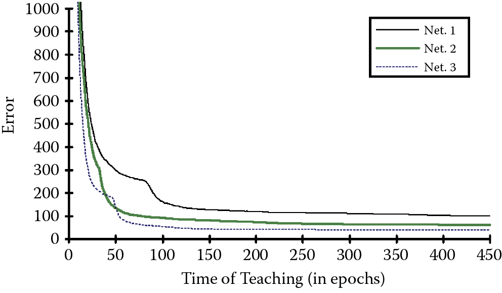
Let us try to check the progress of the teaching process in your experiments. You will obtain different characteristics of teaching in the following experiments despite using the same set of input data. The reason is that a neuron starts from a different randomly drawn initial weight value every time it operates.

The Example 03 program is user friendly. It will allow you to experiment with a neuron by interrupting teaching to examine the neuron and see how it behaves after using trial signals that are similar to the signals it was taught. You can then return to the interrupted teaching process to “tune up” the neuron, then examine it again. You can teach a neuron a few rudiments, examine it, teach it again, check its progress, and so on. We suggest successively longer periods of teaching between examinations because changes over time become less noticeable.

Experiments are worth conducting because they produce substantial and detailed information. Furthermore, they are based on simple examples that demonstrate the most impressive feature of a neural network—its ability to learn and generalize great amounts of data.

5.3 “Inborn” Abilities of Neurons

It is advisable to understand how “inborn” abilities influence teaching effects. To achieve this aim, you should repeat the teaching process several times by starting the program from the beginning and observing the changes that occur. Random setting of initial weight values will enable you to observe different paces of teaching neurons using the same input data. Some neurons learn instantly and some require lengthy teaching. Neurons occasionally produce unsatisfactory results despite intensive teaching. This occurs when they must overcome “inborn preferences” while learning.

This effect may be surprisingly large. We suggest readers conduct a few experiments with the suggested program by changing the range in the text of program where initial random weight values are set.* You start by setting initial parameters of weight neuron value other than those assumed in the InitializeTeaching () klasy ProgramLogic method. Instead of using examinedNeuron.Randomize(_randomGenerator, -0.1, 0.1), you can apply the _examinedNeuron.Randomize(_randomGenerator, -0.4, 0.4) instruction.

The initial weight values will undergo a wider range of changes and thus exert more influence on teaching and on the results. By starting the teaching process several times with the same data, you can easily observe how strong the influence of the random initial weight value is. The neuron will learn in a completely different way every time. You will be able to recognize the unpredictability of the learning process and its results as well.

The network used in the experiments described in this chapter is small and simple. Its assigned task is not difficult. If you are solving very complex tasks in a large network, the addition of many random effects (investigated in the described program) can lead to unforeseen network behavior. The effect may amaze users who trust the infallible behavior repetition of numeric algorithms used in typical computer programs.

5.4 Cautions

The simple demonstration suggested above can act as a testing ground for investigating one more important factor influencing the teaching process, namely the influence of teaching ratio value (pace) on the outcome. This factor can be changed in the teaching ratio field of the Example 03 program.

By assigning a larger value, for example, using a ratio of 0.3 instead of the 0.1 used in the program, you can get faster teaching results, but the network may become “nervous” because of sudden weight value changes and unexpected fluctuations. You can try to use a few new values and observe their impacts on the teaching process.

If you set too high a value of a factor, the teaching process becomes chaotic and does not yield positive results, because neurons will be “struggling” between extremes. The final result will be unsatisfactory. Instead of improving its results, a neuron working with values set too high will generate many more errors than expected.

On the other hand, a too-low teaching ratio value will slow teaching considerably. The user will become discouraged by the lack of progress and abandon the method to seek more effective algorithms. All experiment results on artificial neural networks should be interpreted in light of situations that arise in a real teaching process. The teaching ratio value expresses “strictness” of a teacher to a neuron. Low values indicate a lenient teacher who notices and corrects teaching errors but does not demand correct answers. As shown in earlier experiments, such indulgence can yield poor results.

A very high teaching ratio value is equivalent to a too-strict teacher and this extreme may be detrimental also. Very strict punishments imposed on an apprentice after a mistake create frustration. The situation is the same as a neuron “struggling” from one extreme value to another without making real learning progress.

5.5 Teaching Simple Networks

The natural course is to proceed from teaching a single neuron to teaching an entire network. The Example 04 program is designed for this purpose. It is similar to Example 03 designed for a single neuron and is also easy to use. You also need teaching set data to conduct experiments with this program. It is available in the Default teaching set 04.txt file. The content of the teaching set appears below:

5, 3

A typical object that should be accepted by the first neuron is

3, 4, 3, 4, 5

1, –1, –1

A typical object that should be accepted by the second neuron is

1, –2, 1, –2, –4

–1, 1, –1

A typical object that should be accepted by the third neuron is

–3, 2, –5, 3, 1

–1, –1, 1

An untypical object that should be accepted by the first neuron is

4, 2, 5, 3, 2

0.8, –1, –1

An untypical object that should be accepted by the second neuron is

0, –1, 0, –3, –3

–1, 0.8, –1

An untypical object that should be accepted by the third neuron is

–5, 1, –1, 4, 2

–1, –1, 0.8

An untypical object that should be rejected by all neurons is

–1, –1, –1, –1, –1

–1, –1, –1

The program indicates the state of teaching process and values of particular variables with a little less detail than that shown in Example 03. Using a larger number of neurons generates a too-precise view of each neuron’s results. In essence, you would receive too much information and find it difficult to extract the essential data from the results. The insights provided by Example 04 program are more synthetic. Results from three neurons are apparent instantly, as shown in Figure 5.8.

The critical aspect of teaching is progress of the learner. You can view the progress of the teaching process by comparing Figure 5.8 and Figure 5.9 that depict network condition at the beginning and end of teaching, respectively.

The Example 04 program shows network behavior (Figure 5.10) and allows a user to judge whether a network works correctly. The figure indicates that the network after teaching correctly handled an object that was not shown in the teaching data, but is similar to the object the neuron was taught to recognize.

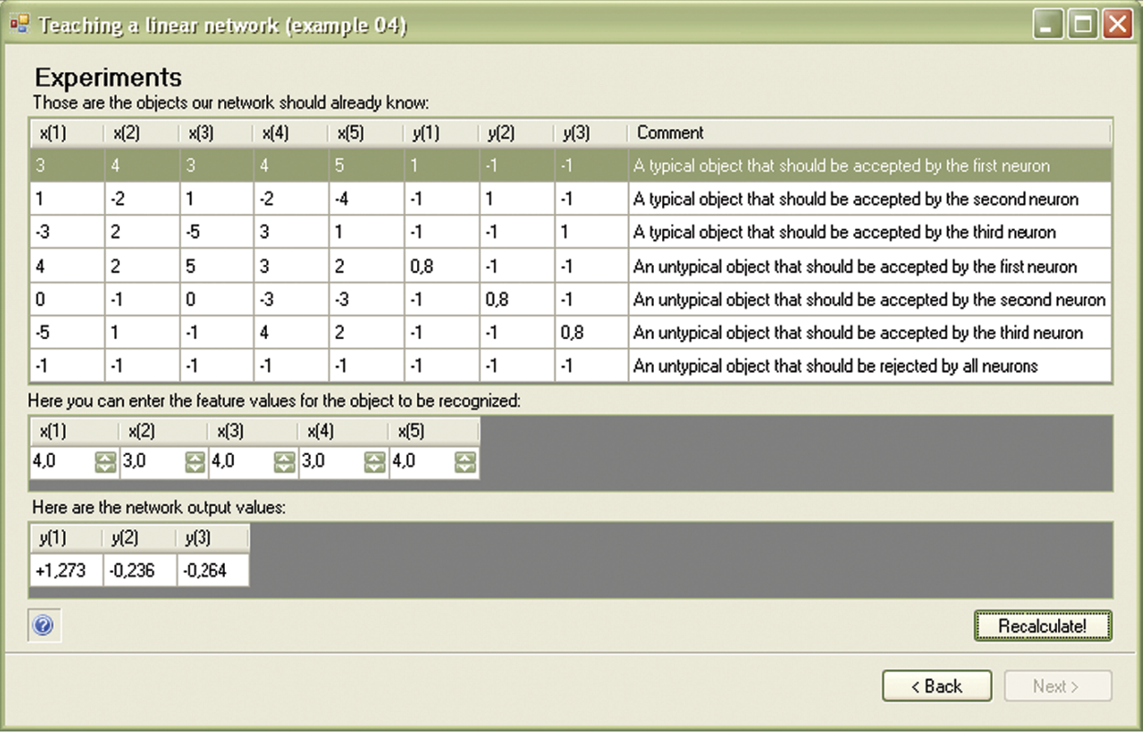
Notice from examination that only the first neuron has a positive value of output signal. This clearly points to the fact that the recognition process proceeded successfully. However, the ambiguity of this situation caused Neurons 2 and 3 (that should have rejected the object) to have doubts indicated by their uncertain answers. This situation is typical.

Utilizing the generalization of knowledge concept during teaching usually allows a user to detect uncertain network behavior. From a neuron’s view, it is easier to achieve success (correct positive recognition) than to strive for certainty and reliability in cases that should have been rejected.

During the observation of network teaching, you can surely notice that some of the demands made in the form of suitable examples included in teaching data are solved easily and quickly and others are far more difficult to solve. The recognition tasks in the Default teaching set 04.txt file are easy for a neuron. However, teaching neurons to reject objects is a more difficult task. Figure 5.11 shows an advanced stage of the teaching process, where recognition of specific objects happens correctly and the object that should be rejected is still causing trouble.

Moreover, repeated unsuccessful attempts of adapting the network to solve this difficult task will lead to deterioration of the current skill of the network for solving elementary tasks. This implies typical object recognition.

If you encounter this situation in practice, instead of struggling and teaching the network unsuccessfully for a long time, consider reformulating the task. It may be more useful to prevent the problem. Usually the removal of one or more troublesome examples from teaching data radically improves and accelerates the process. You can check the extent to which this method improves learning by removing the proper fragment from the Default teaching set 04.txt file and teaching the network again without the troublesome element(s). You will certainly notice an improvement in the speed and effectiveness of teaching.

5.6 Potential Uses for Simple Neural Networks

The networks we investigated in this chapter are not the largest or most complex neurocomputers ever built. For many readers they will appear almost primitive. However, even simple networks show interesting behaviors and are capable of dealing neatly with fairly complicated tasks. This is simply because collective action of many neurons allows a wide range of varied possibilities. We can certainly see some similarities among single neuron activities and network possibilities. Therefore, we can consider a network a set of cooperating neurons. The behavior of a single neuron can be expanded into an entire network in a very natural manner.

However, networks present some uniquely connected possibilities that individual neurons cannot handle. Networks as simple as those described here enable us to solve multidimensional problems that can create serious difficulties for other mathematical and computational systems. To deal with multidimensional problems, we enlarge network dimensions properly by assuming larger values for a number of inputs and outputs to accomplish some practical tasks.

A network can be designed to model complex systems in which many causes (input signals) influence the production of many results (output signals). You can get an idea of the wide range of these applications by accessing the Google search engine and entering “neural networks modeling.” The examples described have been cited almost 30 million times. That indicates huge numbers of practical applications for a single neuron!

Along with creating neuron models of complex systems, we can use simple linear neural networks like those described here for adaptable signal processing. This is another huge area of application revealed by a Google search of “signal processing.”

Digital signal processing led to computer and neuron processing for many more types of signals, for example, speech transmission by phone, pictures recorded by camera or video equipment, modern medical diagnostic technologies, and automatic industrial control and measuring equipment. We should take a short look at this interesting discipline, because signal filtration represents a viable application for neural networks. By filtering signal noises that impede perception, accurate analysis and interpretation of data are possible.

5.7 Teaching Networks to Filter Signals

Imagine that you have a signal containing some noise. Telecommunication, automation, electronics, and mechatronics engineers are challenged daily by such signals. If you ask an expert how to clear a signal from noise, he or she will tell you to use a filter. You will learn that a filter is an electronic device that stops noise and allows useful signals to pass. Because filters work well, we have efficient telephones, radios, televisions, and other devices.

However, each expert will confirm that it is possible to create a good filter only when the noise has some property that is not present in the useful signal. If a signal component has this property, it should be stopped by the filter as noise. Otherwise, the component will be allowed to pass. The technique is simple and effective.

However, to design an effective filter system, you must understand the undesirable noise in your signal. You cannot create a filter without this information because the filter must “know” what information to stop and what to pass Without the necessary knowledge, you will not create a filter, because the filter does not know which information should be kept and which should be stopped. In many cases, you may not know the source of the noise or its properties.

If you send a probe rocket far into space and its mission is to gather signals describing an unknown planetoid, you do not know what rubbish may be attached to signals from the probe during its journey over millions of kilometers. Is it possible to create a filter in this situation?

It is possible to separate a useful signal from unknown noise by using adaptive filtration. In this case, adaptive means teaching the signal receiving device the rules for separating signals from noise. Neural networks can be trained to filter select signals from noise. Samples of disturbed signals are treated as input signals for the network and “clean” signals are used as output signals. After some time, the network will learn to differentiate undisturbed output signals from disturbed ones and will work as a filter.

Let us consider a real example. We will use standard sinusoid signals, both “clean” and disturbed. These signals, in the form of a file that allows to teach networks, can be created by the Example 05 program. This program automatically produces a data file called teaching_set that may be used to teach a simple network. The window for modifying the required parameters to generate this file appears when we start the Example 05 program.

Figure 5.12 shows the window. Unfortunately, the program requires you to input network size, expected noise value (noise level measure), frequency, and number of teaching steps.

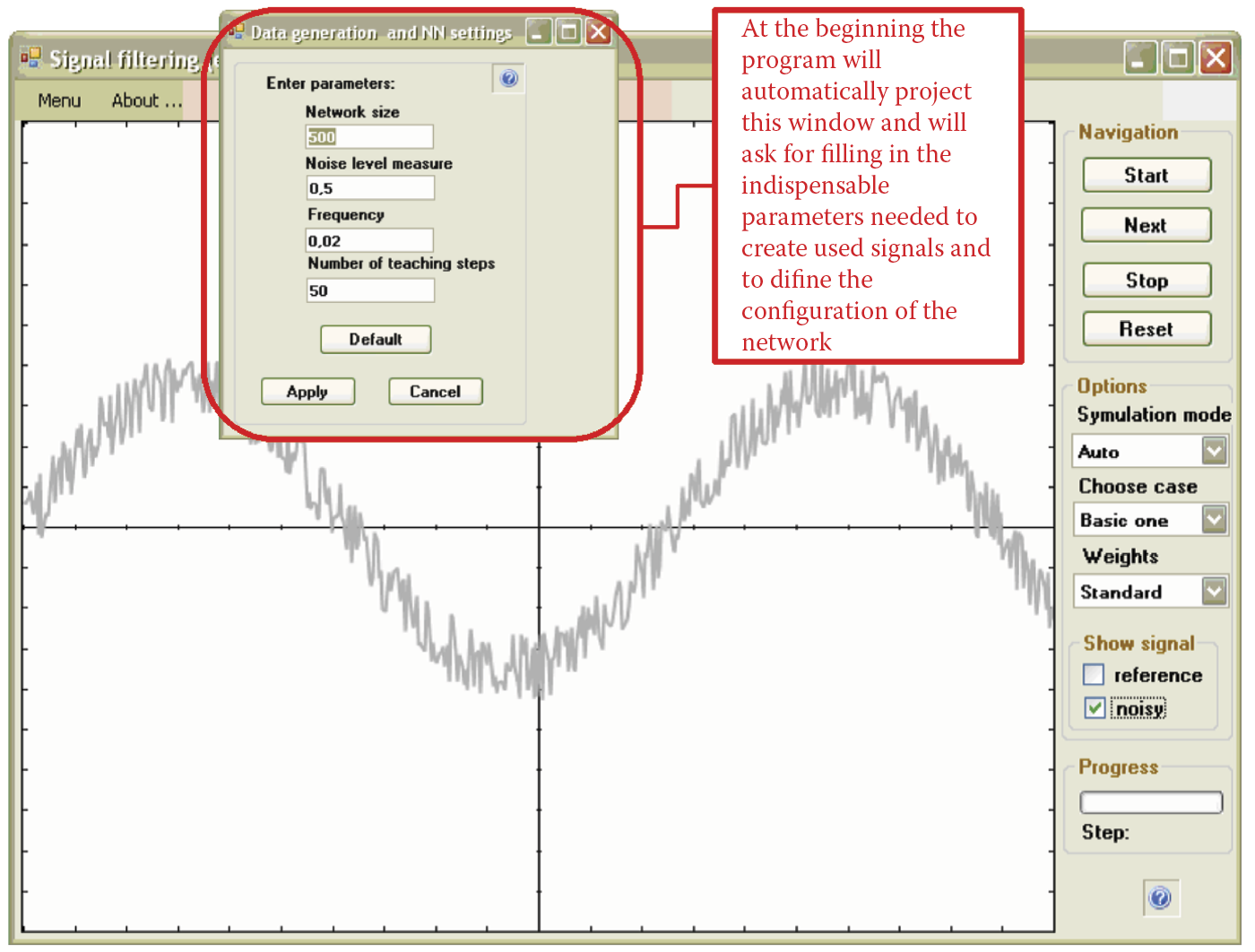
The number of details needed may discourage you from working with this program, but the process of compiling the necessary values is not as complex as it seems.

Each window in the display shows selected values that have been tested to ensure the program works well and produce interesting effects. Therefore, if you do not have values in mind, you can choose the default settings by clicking the Apply button. When you are more comfortable with the program, you can change the values and observe the results.

The Example 05 program provides a great deal of freedom. The default values can be removed at any time by clicking the Cancel button. You can restore all the settings by using the Default button. Although the program appears unfriendly at the start, its operation is straightforward. The system will let you observe as a network teaches itself to filter signals. The program demonstrates all the steps and depicts the unfiltered signal (Figure 5.12) and the post-filtered signal without noise (Figure 5.13). To access these views, select the reference or noisy option from the Show signal group in the right margin displayed on the screen.

The first results of filtration after few steps are not very promising (Figure 5.14 and Figure 5.15), but the constant teaching of the network (by repeatedly clicking the Next button) trains it to filter signals nearly perfectly (Figure 5.16). The teaching process can proceed automatically or step by step. The program allows you to view the various operations or proceed directly to view the filtered signal by making the appropriate choice of simulation mode.

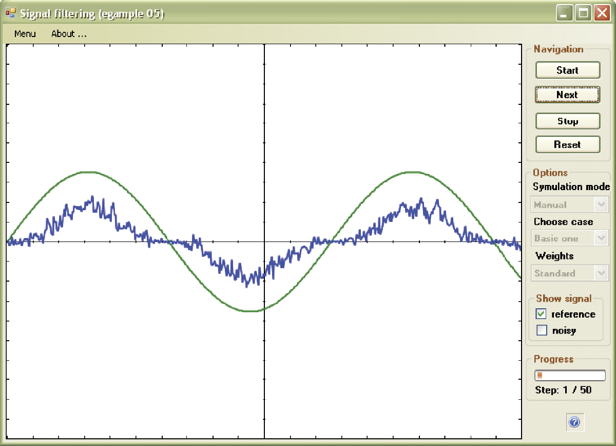
You may find it helpful in early experiments with the program to observe the individual steps of the teaching process by choosing the manual mode. During experiments, it is possible to modify the number of steps (by using the Menu → Configuration option on the upper edge of the window) and use the automatic mode to specify 50 or 100 steps. The results are very informative and worth the effort.

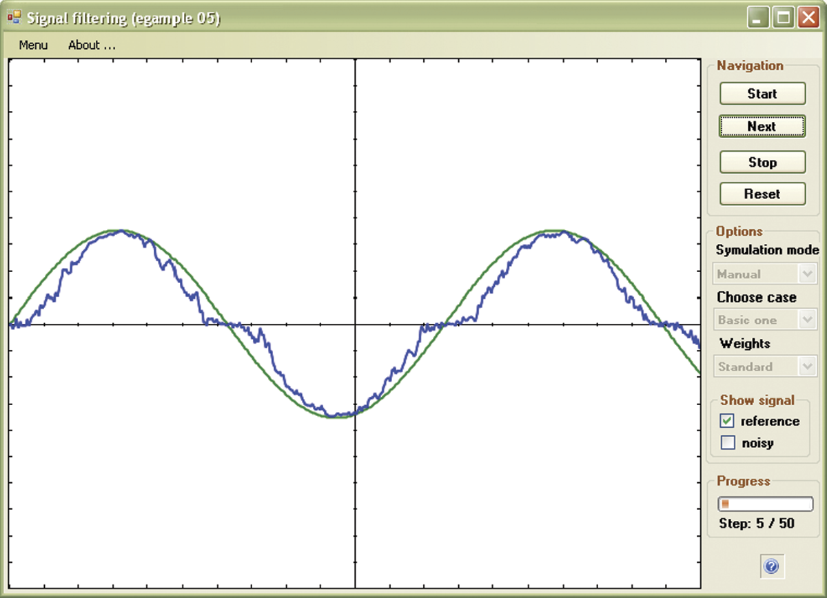
As you can see from the figures, a network really learns and improves its work. After a fairly short time, it erases disturbances in signals easily. The filter effectiveness resulting from teaching can be evaluated by viewing the signal during the process (Figure 5.17). After sufficient teaching, a network learns to filter signals and performs the task well.

The most difficult task is to teach a network to reproduce a signal in a situation in which the values of the standard signals are small or equal zero. Therefore, it is possible in Example 05 to use two versions of network teaching (1) with the original sinusoid signal and (2) after movement of the sinusoidal signal in such a way that the values processed by the network may be only positive.

You select an option from the Choose case menu on the right side. At the beginning, the “with displacement” results appear to be worse (see Figure 5.18). However, persistent network teaching yields much better results (Figure 5.19). The observation of network behavior under all these conditions will help you detect and analyze the causes of possible failures when you use networks to perform far more complicated tasks.

Keep in mind that linear networks represent the “kindergarten” level of the neural network field. Think of the linear network as a warm-up for a big event—creating a multilayer network from nonlinear neurons—the subject of the next chapter.

Questions and Self-Study Tasks

1. Why during network teaching of complicated tasks do we use a teaching set saved on a disk instead of using a mouse or keyboard?

2. Figure 5.4 depicts teaching progress history. Why does it exhibit frequent and sudden fluctuations? Did something cause the neuron to “go crazy” from time to time?

3. Based on the experiments described in this chapter, estimate the degree to which the teaching of a specific behavior exerts influence on the final result. Also, estimate the degree to which a neuron’s “Inborn abilities” resulting from a random initialization of the network parameters influence its work? Do these analyses allow you to draw some practical conclusions about the influence of your education on your career?

4. Try to determine by several experiments using the Example 03 program the best teaching ratio value for the task solved by the network. In another task described by a completely different teaching set, will the optimal value of teaching ratio be the same or different?

5. When should you use larger teaching ratio values: in tasks that are easy to solve or tasks that are difficult and complicated?

6. Try to invent and use another teaching set cooperating with the Example 04 program. Use the Notepad program of Windows or the specialized Visual Study tool. Save the new content in the Default teaching set 04.txt file. Try to master Example 04 until it becomes a valuable tool that enables you to solve various tasks based on a teaching set you randomly select.

7. Prepare a few files with different teaching sets for different tasks and compare the results after a network is taught. Establish the degree of task difficulty (based on the similarities of data sets that the network must distinguish) that influences the duration of teaching and frequency of network errors after teaching is complete. Try to find a difficult task that the network will be unable to learn no matter how much it is taught.

8. Examine how the teaching of the Example 04 program proceeds in relation to initial weight value, teaching ratio, and various modifications of the teaching set.

9. A neural network that learns adaptive signal filtration has at its disposal a signal disturbed by noise and a standard undisturbed signal. Why is the disturbed signal not used as a model during network teaching?

10. Figure 5.18 and Figure 5.19 show that the filtration conducted by Example 05 program is better in the upper part of chart than in the lower section. Why?

11. Advanced exercise: The Example 03 program uses a teaching neural network to create a classifier (a network that receives a specified set of input signals and produces an output signal that could be interpreted as acceptance or rejection of an object described by data). Examine how this program will behave when it is forced to learn a more difficult trick: calculation of a definite output value based on input data values. This network can work as a model of some simple physical or economic phenomenon. The following is an example data set in the form of Default teaching set.txt, for which this model can be created. Only two inputs are assumed in an effort to minimize the use of teaching data.

2, 1

Observation 1

3, 4

–0.1

Observation 2

1, –2

0.7

Observation 3

4, 2

–0.2

Observation 4

0, –1

0.3

Observation 5

4, –5

1.9

Observation 6

–3, –3

0.6

Observation 7

–2, –4

1

Observation 8

3, –2

0.9

Observation 9

–1, –1

0.2

Make sure the program provides correct solutions for a data set other than the one used during teaching, knowing that the teaching data were based on the y = 0, 1 × 1 – 0, 3 × 2 equation.

12. Advanced exercise: The Example 05 program illustrates the work of an adaptive filter based on teaching a neural network instead of a working program designed for practical uses. The same network can be used to filter other signals, for example, electrocardiogram records. This signal in digital form is not at your disposal so try to use a properly modified network for other signals, for example, filter a sample of sound in the form of a WAV or MP3 file. How can a similar adaptive filter network be used for picture processing?

---