
Chapter 6
Nonlinear Networks
6.1 Advantages of Nonlinearity
Linear systems (both neural networks and other linear devices in general) are well known for their predictable nature and use of simple mathematical descriptions to lead easily to solutions. You may wonder why we leave the comfortable area of linear networks and move on to complex nonlinear networks. The most important reason is that networks of nonlinear neurons are able to solve more varieties of problems. Linear networks can solve only a single class of problem—one in which the correlation between output and input signals is linear. Nonlinear networks are far more flexible.
If you are adept at mathematics, you will understand what the problem is, but don’t worry if mathematics is not your strong suit because this book contains no mathematical formulas. And nothing is extraordinary about a network created from linear neurons that deals only with linear functions. One mathematical concept is required here: for a linear transformation, we can use a transformation matrix to obtain an output based only on input signals. Output signals act as vectors. Because that explanation may not be clear, we are going to compare linear and nonlinear transformations by demonstrating their basic properties of homogeneity and additivity (also called superposition).
Homogeneity serves as both a trigger and a result. If an argument is multiplied by a factor, the result is multiplied by some power of the factor. What the cause and result represent in the real world does not matter. If you know a cause, you can predict a result because you understand the rule and the correlation of cause and result.
Multiplicative scaling behavior is, however, not the only possible linear correlation. The real world contains many examples of correlations that do not involve multiplicative scaling. For example, you know that the more you study, the better your grades are; we make a direct correlation between your efforts and your grades. This is a simple type of transformation. However, we cannot say that your grades will be twice as good if you learn twice as much material. In this case, the correlation between efforts and grade is nonlinear because it is not homogeneous.
The other requirement is additivity—another simple concept. When investigating a transformation, you check how it behaves after triggering it and check again after the cause (trigger) is modified. You know the end results for the first and second triggers. The next step is to predict the result if both triggers work simultaneously. If the result is the exact sum of the results we got using triggers separately then the phenomena (and the transformation or function we study) is additive.
Unfortunately, many processes and phenomena that are additive are simply not common in nature. If you fill a pitcher with water, you can put flowers in it. If the pitcher with flowers falls from a table, it will lie there. If you fill a pitcher with water and it falls from the table, you cannot put flowers in it. A pitcher full of water falling from a table will break. The break is thus a nonlinear phenomenon that cannot be predicted as a simple sum of activities that were studied separately.
When creating mathematical descriptions (models) of systems, processes or phenomena, we prefer linear functions because they are easy to use. Linear functions can create simple and efficient networks. Unfortunately, many functions cannot be put into “frames” of linearity. They require complex nonlinear mathematical models. A simpler answer is creating nonlinear neural networks that model the systems, processes or phenomena to be examined. Such neural networks are powerful and efficient tools. A huge multilevel linear network can correlate any types of inputs and outputs as a result of basic mathematical theorems about function interpolation and extrapolation developed by Andrei Kolmogorov, a great Russian mathematician.
We will not go into detail here because the modeling problem is highly theoretical and mathematical. For now, we assure you that the superiority of nonlinear networks over linear ones is a practical problem, not an academic issue. Nonlinear networks can solve many problems that linear networks cannot handle. The program we will study in this chapter will make that point clear. We suggest you experiment with other programs to examine how nonlinear networks work and what they can achieve.
6.2 Functioning of Nonlinear Neurons
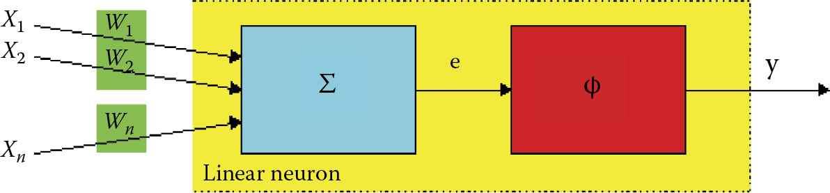
We start with a simple program that shows how one nonlinear neuron works. Figure 6.1 illustrates the structure. The Example 06a program that models a nonlinear neuron is analogous to the Example 01c program we used earlier to explore how a linear neuron works. The Example 06a program will demonstrate step by step how a simple nonlinearly characterized neuron works. It starts by asking the user to choose between unipolar and bipolar characteristics (Figure 6.2) from the Neuron type field. You can set the amount of neuron input, but at this point we recommend accepting the default value of 4 and clicking on the Next button.
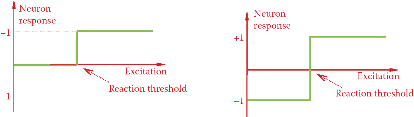
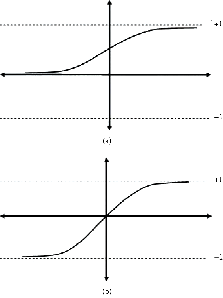
The concept of the unipolar characteristic is simple: the output signal is always nonnegative (usually 1 or 0 and certain nonlinear neurons can yield output values between these extremes). Bipolar characteristics allow a user to obtain either positive or negative signal values (usually +1 or –1, but intermediate values are possible). Figure 6.2 compares unipolar and bipolar characteristics and demonstrates the differences.
We should add one more qualification. Biological neurons such as those in your brain do not recognize negative signals. All signals in your brain must be positive (or zero if you are inactive). Therefore, the unipolar characteristic is more appropriate for achieving biological reality. Technical neural networks are different in that they are intended to act as useful computational tools instead of serving as accurate biological models. We want to avoid situations that allow 0 signals to appear in a network, especially when signals generated by one neuron are treated as inputs for other neurons within the same network. A network learns poorly if it encounters 0 signals. Remember the example of filtering signals discussed in Chapter 5.
The ability of bipolar structures to accept 0 and 1 expands their utility. We also use two other signals labeled +1 and –1. Look more closely at Figure 6.2.
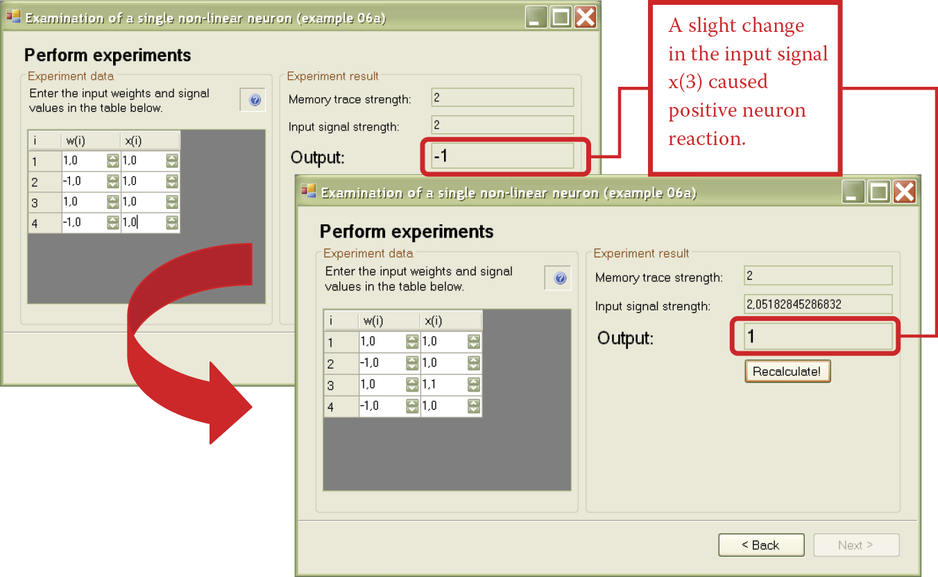
Using the Example 06a program, you will note that nonlinear neurons are more categorical than linear neurons. Figure 6.3 depicts conversations with the program. Neurons and networks react to input signals in a subtle and balanced way. Certain combinations of input signals induce a strong reaction (high output signal), whereas other inputs produce far weaker reactions or cause a network to be almost totally unresponsive when output signals approach 0.
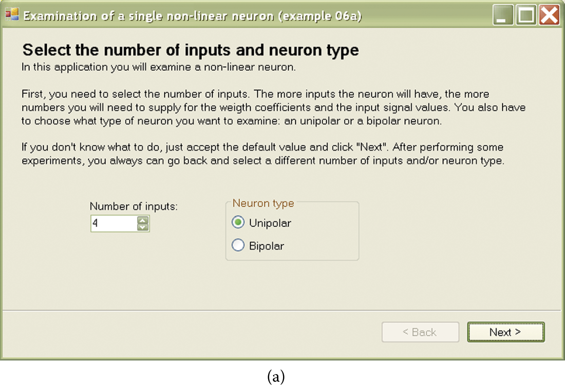
(a) Beginning of conversation with Example 06a program. (b) Next stage of conversation with Example 06a program.
Unlike the subtle linear neurons, nonlinear neurons work on an all-or-none principle. They can react negatively to certain combinations of signals by generating –1 outputs. Sometimes a minimal change in input signals is enough to make a neuron output signal become completely positive and change to +1 as shown in Figure 6.4.
While Example 06a is primitive, its operations are similar to those of a biological brain. A few simple experiments like those carried out with linear neurons will help you to understand how the program works and see how this type of network performs like a real nerve cell.
6.3 Teaching Nonlinear Networks
The Example 06a program involved a neuron whose output accepted two values associated with the acceptance (recognition) of certain set of signals or totally rejected them. This acceptance or rejection limitation is often connected with recognition of an object or a situation. Thus the neurons in the network we examined in Example 06a are often called perceptrons. They generate only two output signals: 1 or 0. In neurophysiology, this choice by a biological neuron is known as the everything-or-nothing rule. The Example 06a program follows this rule and we will use it to build all the networks described in subsequent chapters.
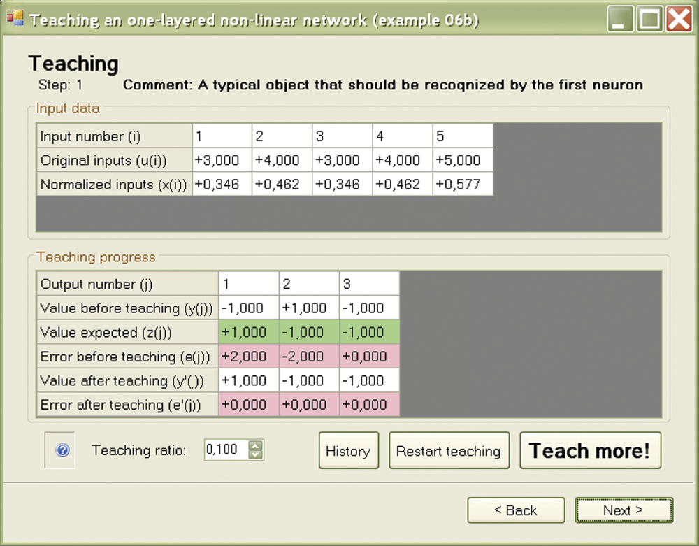
We now consider how to teach and work with a group of bipolar neurons by studying a simple single-layer network of bipolar neurons described in the Example 06b program. To teach a network from this program, you can use the Default teaching set 06b.txt file linked with example 06b. The file may have the following structure:
5, 3
A typical object that should be recognized by the first neuron is
3, 4, 3, 4, 5
1, –1, –1
A typical object that should be recognized by the second neuron is
1, –2, 1, –2, –4
–1, 1, –1
A typical object that should be recognized by the third neuron is
–3, 2, –5, 3, 1
–1, –1, 1
Contents of a similar file were discussed in Chapter 5 so we will not repeat the details here. You can review Chapter 5 if you need clarification. Comparing the above file to the one used earlier, we observe that a small number of examples is sufficient because a nonlinear network can learn very quickly. Usually only one step of learning is sufficient to eliminate errors (Figure 6.5). On average, a nonlinear network is taught fully after six or seven steps and is ready for examination. These networks learn quickly and thoroughly.
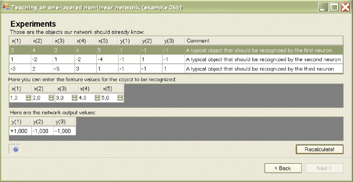
The effect of the knowledge generalization in neural networks is an important issue. What would be the benefit if you taught a neural network a series of tasks with the correct solutions and later find that it is unable to solve tasks beyond those it learned earlier? What you really need is a tool that learns to solve tasks from a teaching set and later can be used to solve other tasks by applying knowledge generalization. Knowledge generalization means that learning on a limited number of examples not only gains the knowledge necessary for solving these examples, but also can solve other unknown problems similar to those used during learning.
Fortunately, neural networks can generalize knowledge (Figure 6.6) and skillfully solve tasks similar to those included in a teaching set if the tasks are based on the similar logic of the relationships between inputs and outputs. Generalization of knowledge is one of the most important features of neural networks. For that reason, we encourage you to change input data on which teaching is based. We recommend that you try to “bully” a nonlinear network in various ways to assess its capabilities and compare its performance with performances of linear networks.
6.4 Demonstrating Actions of Nonlinear Neurons
The outputs of neural networks built from nonlinear neurons can be interpreted easily by drawing the so-called input signal space and indicating which values of the signals trigger positive responses (+1) and which ones trigger negative responses (–1) of neurons. Assume we want to interpret input signal space data.
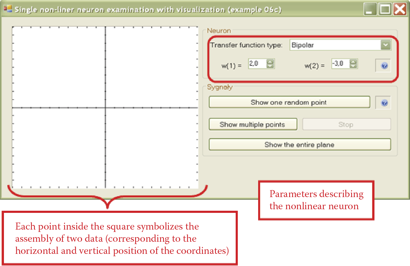
Each point inside the large square created by Example 06c represents a set of data (equivalent to the horizontal and vertical coordinates of the position of a point) composed of input signals of a neural network. The analyzed network is the brain of a hypothetical animal equipped with receptors for sight and sound (Figure 6.7). The stronger the signal received by the sight receptor, the more the point drifts to the right. The stronger the sounds are, the higher the location of the point.
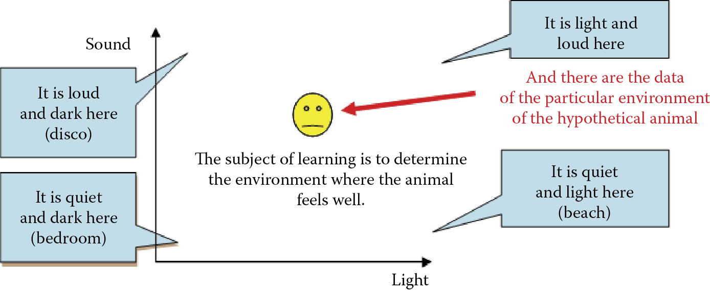
Experimental world of a hypothetical animal with a neuron brain containing receptors for sight and sound.
The bottom left corner of the figure represents the conditions of silence and darkness (bedroom). The upper right corner indicates maximum sound and light conditions, for example, in a city’s main square at noon. The upper left corner may represent a disco because conditions are dark and loud. The bottom corner is sunny and quiet, like a beach. You can imagine similar analogies for other points in the square. All the situations in the figure can be perceived by the hypothetical animal as positive (the point will show intense red color) or negative (blue); see Figure 6.8.
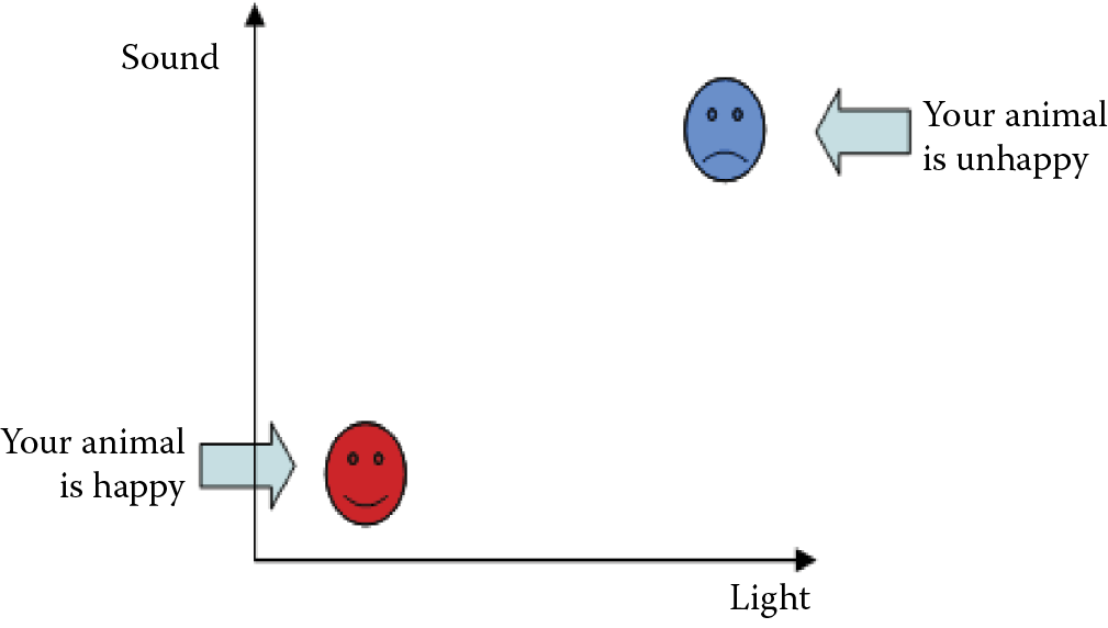
Imagine that the brain of our modeled animal consists of a single nonlinear neuron. Obviously, the neuron must have two inputs to accommodate the receptors for sight and sound. The two weights must be determined for each receptor. For example, when the first weight (sight) is positive, the animal may like lighted surroundings. A negative value may cause the animal to hide in a dark corner. The same procedure can be used with the second weight (sound), allowing you to determine whether the animal prefers peace and quiet or heavy metal concerts.
After your animal is programmed, it will be tested by exposure to different combinations of two input signals. Each initial combination of signals can be treated as an indication of a specified environment where the animal is placed. The properties of this environment are symbolized by a point on the plane of the picture. The value of the first signal (lighting) indicates the x axis of the point. The value of the second signal (sound) is the y axis. The neuron makes its decision based on the basis of input signals. A +1 indicates a type of environment will be accepted by the animal; –1 indicates rejection by the animal.
Try to prepare a map depicting the preferences of your neuron by coloring the points accepted by the neuron (+1 output) in red and indicated the rejected (–1) points in blue. The Example 06c program will perform this exercise for you. You must first provide all the weights to define the preferences of your neuron (Figure 6.9). You can then check the values (+1 or –1) generated by the neuron at its output at specific points on its input signal plane. The program is very useful because it performs calculations, draws a map, and generates the required input signals for neurons and provides their coordinates (Figure 6.10).
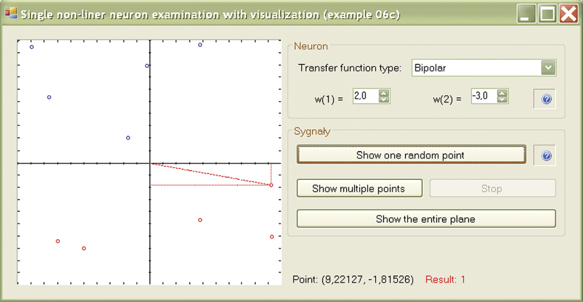
If you want to monitor the positions of new points on the screen, you can press the “Show one random point” button. A currently generated point is already marked by its coordinates projected onto the axes so it can be easily distinguished from the points generated earlier. While checking the position of a new point, you may wonder why the neuron accepted or rejected it. Data for the present point are shown on the line below the picture. Many points will be needed to create a map that would indicate precisely the areas of input signal planes where the responses were positive and negative. Pressing the “Show multiple points” button will switch the program into continuous mode in which the subsequent points are automatically generated and displayed on the map. You can always switch back to the previous mode by aborting the process with the Stop button. Eventually, the outline of the areas with the positive and negative responses of the neuron will appear (Figure 6.11).
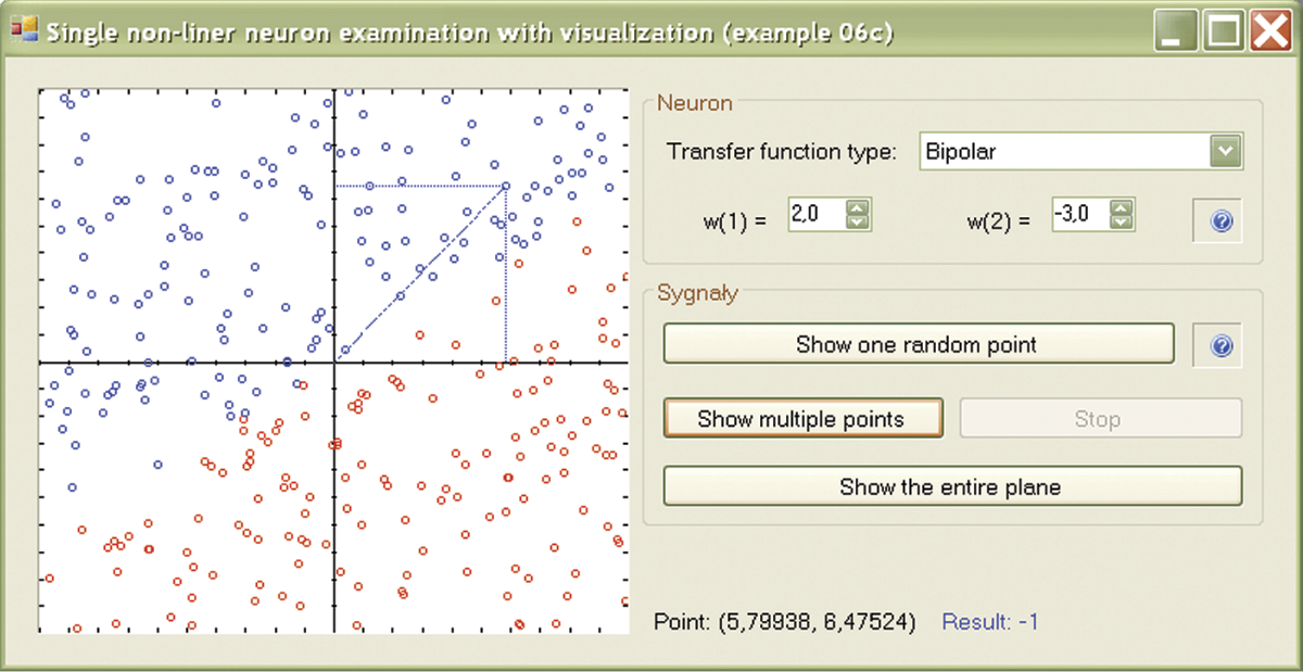
The border between these areas is clearly a straight line; it may be said that a single neuron performs a linear discrimination of the input plane. However, that statement refers only to what you will see on the screen while conducting the experiments described here.
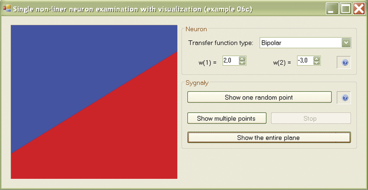
If you wish to see the map of the neuron response without the effort of generating the points, the Example 06c program allows you to do so by using the “Show the entire plane” button (Figure 6.12). One interesting experiment is to change the nonlinear characteristic of a neuron by choosing another option from the “Transfer function type” list.
6.5 Capabilities of Multilayer Networks of Nonlinear Neurons
One neuron (or one layer of neurons) may distribute two input signals by the boundary line in two-dimensional space as a straight line. By appropriately combining such linear bounded areas and properly juxtaposing them, you can obtain virtually any values of aggregated output signals at any points of input signal space. The neural network literature often contains the somewhat misleading claim of using neurons to generate arbitrarily accurate approximations of all kinds of functions.
This is not possible for a single layer of neurons, as shown by theorems of Cybenko, Hornik, Lapedes, Farber, and others. Scientific reason indicates that the use of multiple layers is necessary in such cases because structural elements forming the desired function built by learning neurons must be collected at the end by at least one resulting neuron (usually linear). This means that networks described as universal approximators in fact contain at least two and often three layers.
Bold statements that networks can approximate any function irritate mathematicians who then attempt to devise functions that neural networks cannot master. The mathematicians are correct in that a neural network does not have a chance with certain types of operations but nature is more generous than mathematicians. Real-world processes (physical, chemical, biological, technical, economic, social, and others) can be described by functions that exhibit certain degrees of regularity. Neural networks are able to handle such functions easily, especially if they consist of multiple layers.
Clearly a network consisting of multiple layers of neurons has much richer potential than the single-layer network discussed above. The areas where neurons will positively react to input signals can have more complicated forms. Two-layer networks contain convex polygons or their multidimensional counterparts called simplexes. Neural networks with more layers may contain both convex and non-convex polygons or even connected areas composed of many separate “islands.”
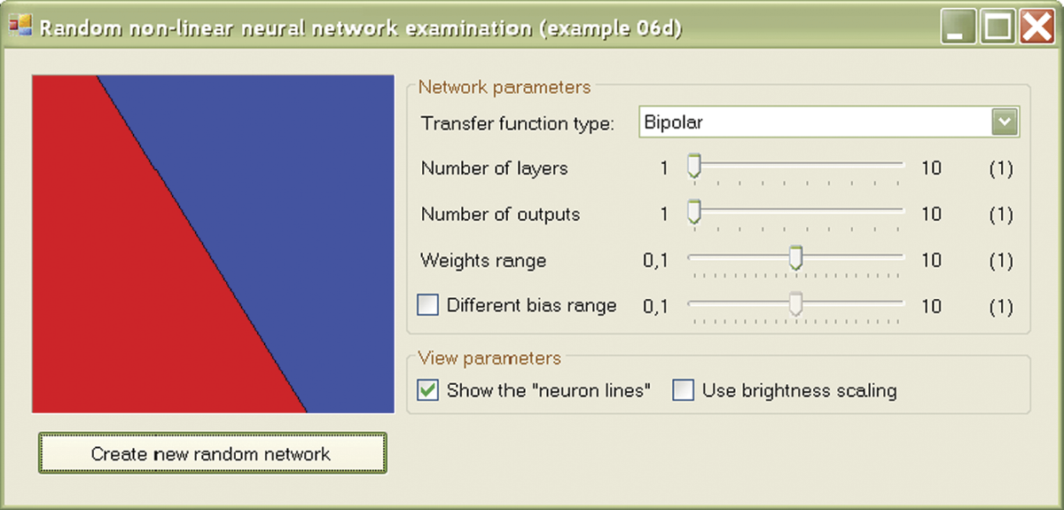
The Example 06D program illustrates this situation. This program allows you to obtain maps such as those built in the previous program faster. Most important, the program works for networks with any number of layers. If you choose a single-layer network, you will see the familiar image of linear discrimination (Figure 6.12).
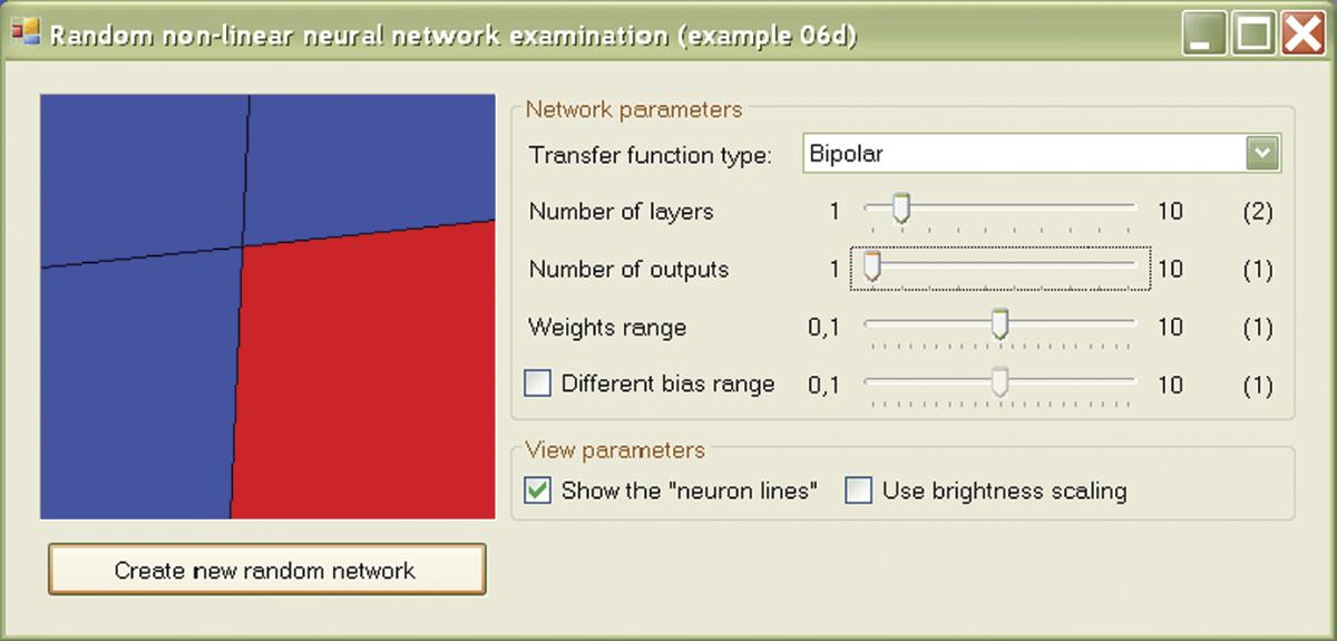
If you choose a two-layer network, you will see that the network can cut out the connected subspace convex bounded by planes (simplex) in the input signal space (Figure 6.13). A network with three or more layers has no such limitations. The area highlighted by the network in the input signal space can be complicated, not necessarily convex, and not necessarily connected (Figure 6.14). By using Example 06d, you can examine a lot more areas because the program randomly uses properties of the network. This enables you to view variants of the shapes described above.

It is also possible to change the network parameters, including the number of layers, neuron activation function (select Transfer function type), and number of network outputs. The network has other interesting features beyond the scope of this chapter. We encourage you, however, to try and discover all the potential of this program. If you are interested in programming, we encourage you to analyze its code because it is a good example of the art of programming.
Figure 6.15 and Figure 6.16 produced by this program clearly show how the growing number of network layers increases a system’s ability to process input information and implement complex algorithms expressing the relationships of input and output signals. These phenomena did not occur in the linear networks we discussed earlier. Regardless of the number of layers, a linear network realizes only linear processing operations of input data into output data so there is little need to build multilayer linear networks. The picture is quite different for nonlinear networks in which increasing the number of layers is a basic operation intended to improve the functioning of the network.
6.6 Nonlinear Neuron Learning Sequence
We now consider the geometrical interpretation of the learning process of a nonlinear neural network. We start from the simplest case—the learning process of a single neuron. As we know, the action of such a neuron is to divide the region of input signals into two regions, In a flat case (e.g., a typical two-dimensional Cartesian space), the linear function will be a straight line but interesting structures will appear in the n-dimensional space. They are affine varieties of the n – 1 order or simply hyperplanes. Such surfaces must be precisely to separate input points for which the network should give contradictory answers.
The Example 06e program will allow you to see how learning of a nonlinear neuron takes place and how the boundary is changed automatically from the random position set at the beginning to the optimum location to separate two groups of points for which the conflicting decisions were applied during the learning process.
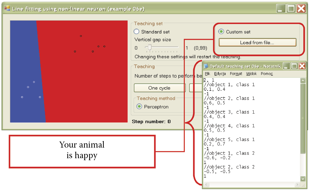
The initial screen of the program shows two sets of points (10 objects each) for sequence learning. Points belonging to one set are shown as small black circles. The second set points are shown as white circles. The collection consists of two clearly separate clusters, but to make the task more difficult, each set contains a single “malicious” point located in the direction of the opposite set. Fitting the boundary line, first between sets, and then more precisely between the “malicious” points located close to each other, is the main task of the learning process. The positions of these points may be adjusted freely by creating an input data file in the Example 06e program, then choosing “Custom set” option in the teaching set to load it (Figure 6.17). An example is presented in the Default teaching set 06e.txt file.
Selection of custom set of data from user’s file together with example of content of user’s data set file for Example 06e.
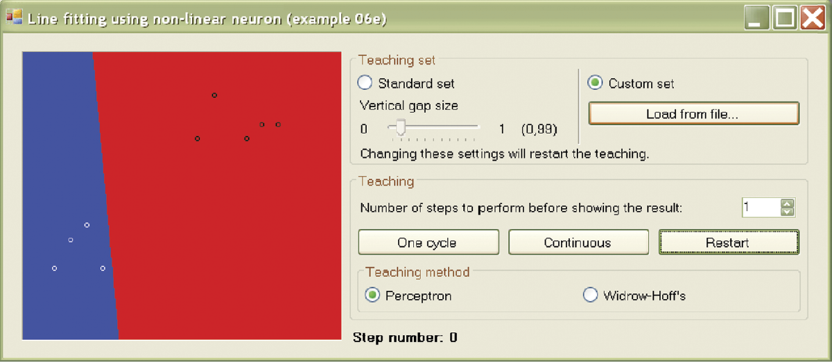
At the beginning, it will be comfortable to run the program with default parameters (Standard set). A slider option allows a change of set location (Vertical gap size). A closer location makes the neuron’s task more difficult. When you select Standard set and run the program, you will see the screen shown in Figure 6.18.
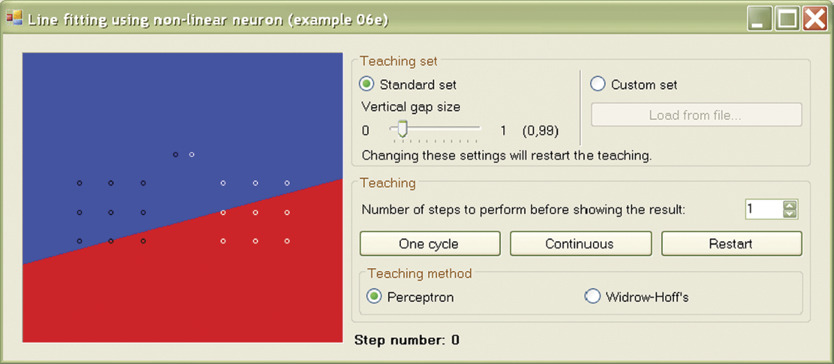
Initial state of learning process in Example 06e program after selection of Standard set option for input data.
The image shows the points mentioned above and the initial random position of the boundary line at the junction of two half-planes marked with different colors. Of course, the initial position of the boundary line depends on the initial parameters of the neuron. As usual with learning tasks, the neuron’s job is to adjust the weights so that its output is consistent with the qualifying points of the training set given by the teacher.
On the screen, you can see the fixed locations of both sets of points on which the neuron is trained, and also the position of the boundary line that changes during learning. The initial position of this line comes from the assignment of random values to all neuron weights. Such initial randomizing of weight is the most reasonable solution since we have no idea which weight values will be appropriate for the proper solution. Thus we cannot propose a more reasonable starting point for the learning process. For this reason, we cannot predict the location of the line separating our points initially and after modification resulting from learning.
By observing how the line gradually changes position and “squeezes” between the delimited sets of points, you can learn a lot about the nature of learning processes for neurons with nonlinear characteristics. Each time you click the “One cycle” button, learning of the desired number of steps in the cycle occurs.
You can change the number of learning steps performed in a single cycle before the next display of the boundary line. This feature is very practical because learning is characterized by rapid progress at the beginning (consecutive learning steps easily shift the boundary line); subsequent progress is much slower. We recommend setting smaller numbers (1, 5, or 10) at the beginning. Later you will have to set “jumps” of 100 and of 500 steps of the learning process between consecutive shows (Figure 6.18).
You do not have to constantly click the “One cycle” button. Pressing the “Continuous” button will instruct the program to follow one cycle until the button is pressed again. The program displays how many learning steps were performed. See the “Step number” feature at the bottom of the application window that allows you to monitor the learning process.
As seen in Figure 6.18, the initial position of the boundary line is far from the target location. As expected, one side of the boundary line displays all points belonging to one set and the other side indicates all points of the second set. The first learning stage (Figure 6.18) is very short—only three shows—but produces noticeable improvement. This trend continues through subsequent steps as more points are separated (Figure 6.19). Unfortunately, Step 51 reveals deterioration of learning and more points are located on the wrong side of the boundary line. The network performance deteriorated after it encountered the “malicious” points that are very difficult to separate from points in a set of easily distinguishable data. The next 10 steps fix this crisis in the learning process and generate significant improvement.
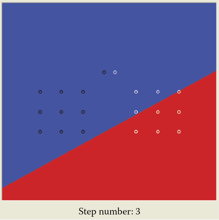
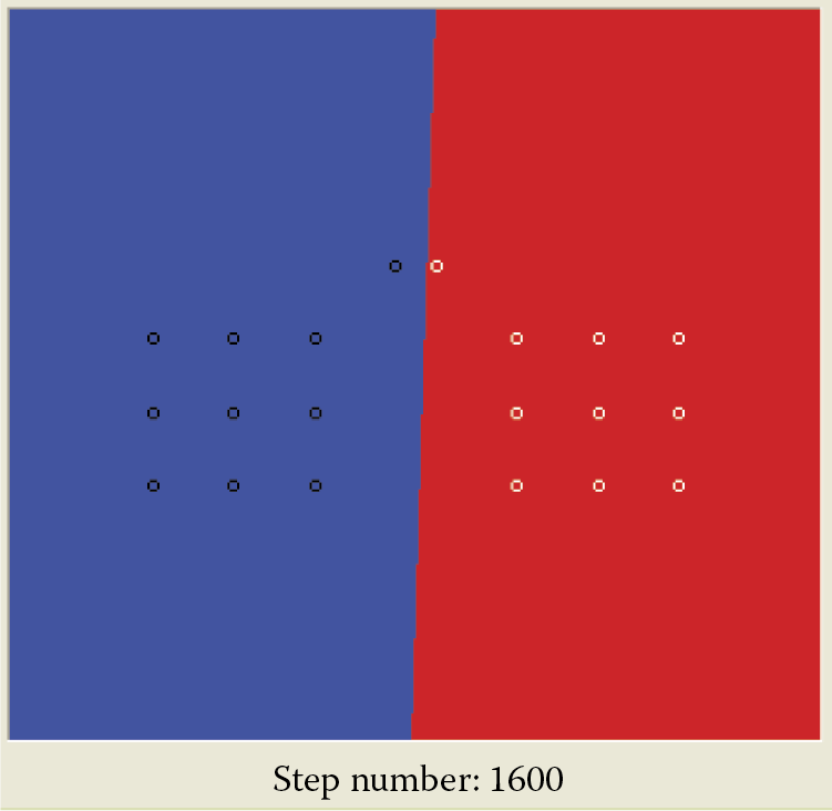
Figure 6.20 indicates that learning is finished and was successful because the final line (on the boundary of the red and blue half-plane) separates the set of points ideally. Note that after a network reaches a correct solution, continued learning will not yield anything new. For example, the lines shown after 1600 and 3600 steps of learning are the same. This is natural, because after learning a neuron does not modify the proper (determined by point qualification) values of the weighting factors.
6.7 Experimentation during Learning Phase
Example 06e allows you to conduct experiments in various ways. After you set up the data of interest and the desired parameters, you can change the positions of the individual points or even entire learning data sets. You can also apply one of the learning methods for nonlinear neurons described in the literature: the perceptron based on output signal and its confrontation with the learning data set or the Widrow–Hoff technique that assumes that learning is performed only for linear parts (net value-based learning). You can select one of these from the Teaching method list.
By conducting your own research, you can demonstrate that the Widrow–Hoff method named for its inventors is more robust in some cases. After a few attempts, you will find that almost ideal separation will be achieved more quickly by the Widrow–Hoff method than by the perceptron. The Widrow–Hoff method never stops learning. After finding a correct solution, it reviews it, repairs it, and continues the process.
People behave similarly. Aleksander Gierymski, a famous Polish painter, was never satisfied with his work. After painting masterpieces, he was obsessed with improving them. He erased objects, added new ones, and continued modifying his paintings until they became worthless. The only remaining works of this great artist were rescued by his friends who forcibly took them—unfinished—from his atelier!
Questions and Self-Study Tasks
1. List at least three advantages that justify the use of nonlinear neurons in solving complex computing tasks.
2. Do linear neurons have unipolar or bipolar characteristics (transfer functions)?
3. What are the benefits of the bipolar transfer functions of neurons? Are they present in the brains of humans and animals? Why?
4. Two commonly used neuron transfer functions are shown in Figure 6.21. Which one is unipolar and which is bipolar?
5. What is the generalization of knowledge phenomenon observed in neural network learning?
6. What limitations must be taken into account for tasks that can be solved by neural networks of (a) a single layer, (b) a double layer, and (c) three layers?
7. Based on experiments with the classification of points belonging to two classes of sketch graphs, show how the error rates of networks change as they learn.
8. What conclusions do you draw by analyzing the shape of the graph obtained by answering Question 7?
9. Why do repeated learning attempts by the same network based on the same training data usually result in variations of learning processes?
10. Advanced exercise: Try to justify the theorem (which is true) that linear networks with multiple layers can achieve only the same simple mapping of input data to output results as a one-layer network. The conclusion (also true) is that a multilayer structure for a linear network produces no advantage.
11. Build a program that will teach multilayer neural networks to recognize classes built from points placed arbitrarily on the screen by clicking the mouse at certain positions.
12. Build a program that allows a network to classify the input points in five (rather than two) classes as shown in the program used in this chapter.