
Chapter 9
Self-Learning Neural Networks
9.1 Basic Concepts
We have explained the structures and utilized programs to demonstrate how a neural network utilizes a teacher’s guidelines for pattern recognition and comparison to complete its tasks. This chapter will detail network learning without a teacher. We discussed self-learning networks briefly in Section 3.2 in Chapter 3. We will now discuss these networks in some depth.
We will not examine the common self-learning algorithms devised by Hebb, Oji, Kohonen, and others in great detail or discuss their mathematical bases. We will explain their operations and uses, and utilize examples to demonstrate their workings. We suggest you start by running the Example 10a program.
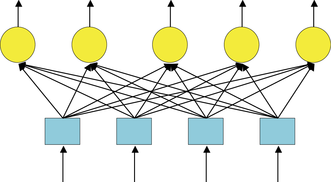
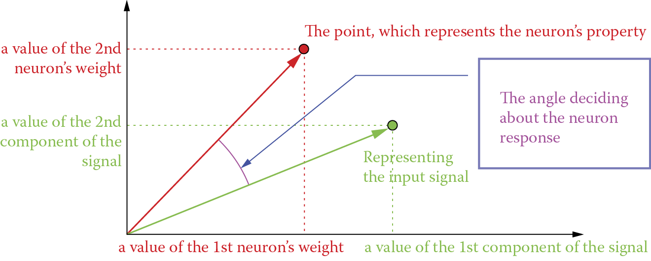
The program deals with a single-layer network of neurons (Figure 9.1). All neurons are given the same input signals, and each one determines independently of the others the value of its degree of excitation and multiplies its input signals (the same for all neurons) by its individual weighting factors (Figure 9.2).
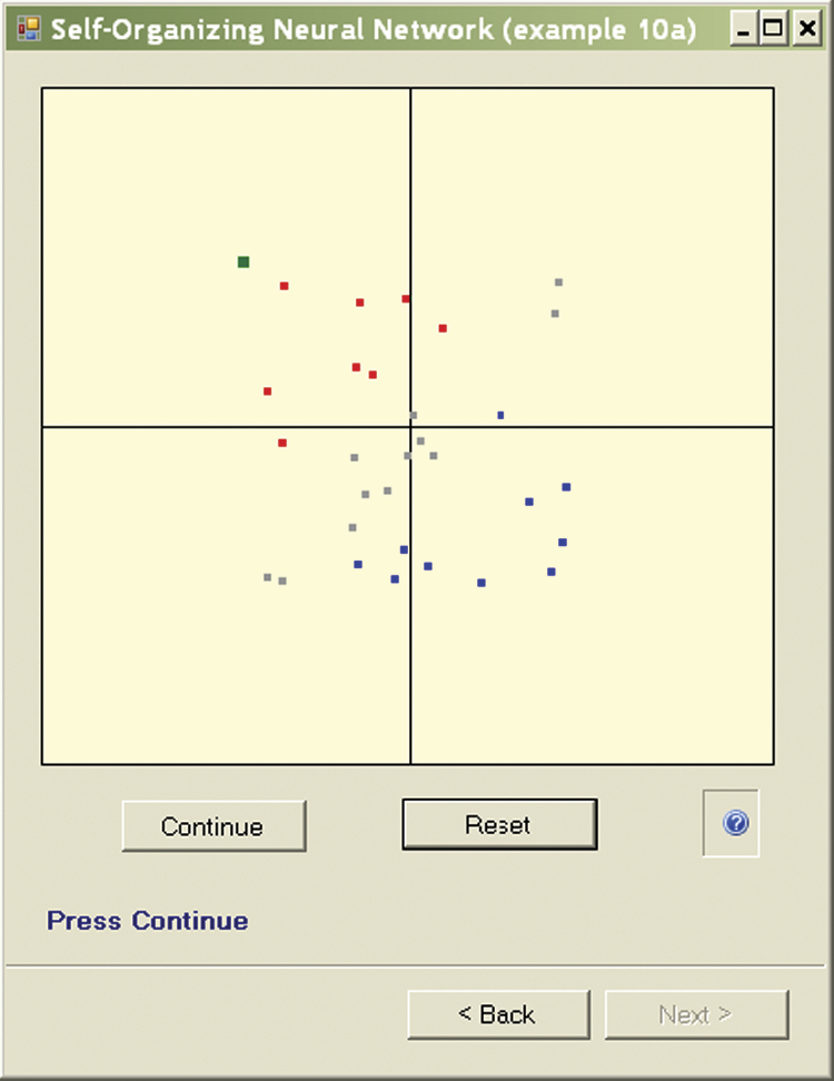
The self-learning principle requires that all neurons at the beginning obtain random weighting factor values that appear in the figure produced by the Example 10a program as a “cloud” of randomly scattered points. Each point represents a single neuron and the point locations are determined by the weighting factor values as shown on the right side of Figure 9.3. The window on the left side of the figure, as in previous programs, appears soon after start and serves to modify network parameters.
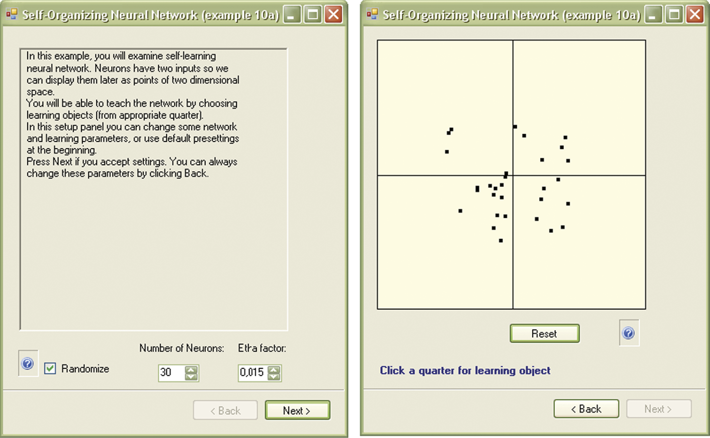
Initial window showing parameters (at left) and locations of points representing neurons after Example 10a program is run.
Set-up requires two parameters: the number of neurons in the network and a parameter named etha that represents the intensity of learning (higher values yield faster and more energetic learning). You may change these parameters at any time. However, at this stage we suggest you accept the default settings we selected after studying program behavior. We will return later in this chapter to descriptions of individual parameters and experimenting with their values.
After starting the program you will have a network composed of 30 neurons characterized by a moderate enthusiasm for learning. All the weights of all neurons in the network will have random values. To begin, we enter input signals that are examples of sample objects the network will analyze. Remember the Martian example in Chapter 3? Entering these objects in the Example 10a program will produce an impact. This contradicts the idea of self-learning that requires the user to do nothing. While the process of learning can proceed independently of user actions, we devised Example 10 intentionally to deviate from the ideal to demonstrate how the presentation of learning objects affects independent knowledge acquisition by a network.
However, some explanation is needed. All the knowledge the network can gain during self-learning comes from the objects presented to it at the input and also from the similarities among classes of objects. Thus, some objects are similar to each other (Martian men) and belong to another class (Martian women) because they are different. Therefore, neither you nor the automatic generator can prevent the network from showing objects that are distributed randomly in the input signal space. Presented objects should form explicit clusters around certain detectable centers that can be named and interpreted (typical Martian man, typical Martian women, etc.).
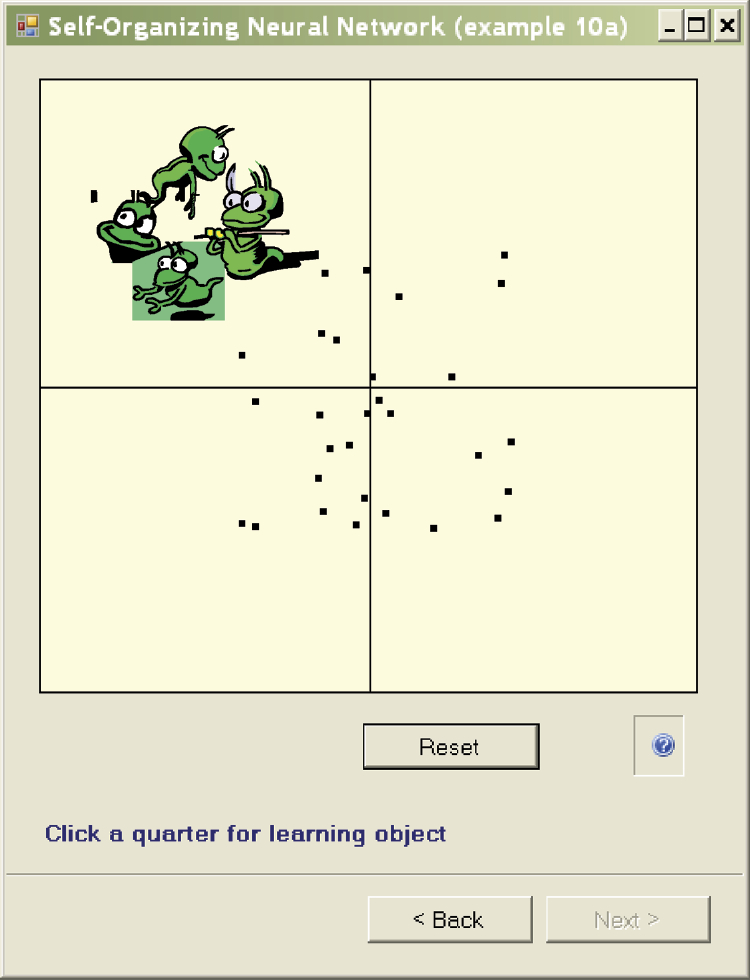
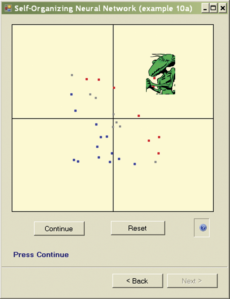
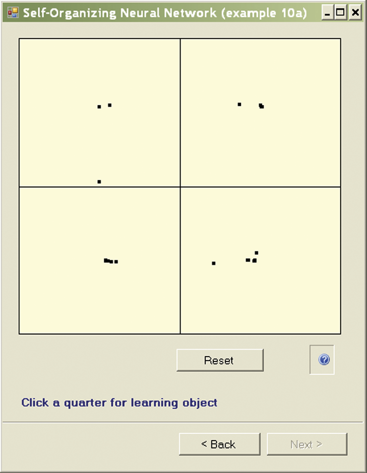
While working with Example 10a, you may decide each time what to show to the network, but your choice will not be fine-tuned because the details will be determined by the system. You will be able to indicate the quadrant* within which the next presented object should be located. All you have to do is to click the mouse on the right quadrant to control what the network will “see.” For example, the objects in the first quadrant belong to the Martian men; the second quadrant is for Martian women, the third to Martian children, and the fourth to Martianamors.† With a little imagination, you can see the window displayed by Example 10a in a manner (Figure 9.4) that shows Martians in sketch form instead of points representing their measured features.
As you can see, every Martian is a little different but they have certain similarities and therefore their data are represented in the same area of the input signal space (this will help a neural network learn how a typical Martian looks). However, since each Martian has individual characteristics that distinguish him, her, or it from other Martians, the points representing them during self-learning will differ little bit. They will be located in slightly different places within the coordinate system. However, since more features distinguish Martians generally than features that distinguish each of Martian individually, the points representing them will concentrate in certain subareas of input signal space.
Generating objects used in the learning process will enable you to decide whether to be shown the Martian man, Martian woman, Martian child, or Martianamor. You will not need to provide details such as eye color because the program will find them automatically. At each learning step, the program will ask you about Martian type—the quadrant to which the object belongs. After you choose one quadrant, the program will generate an object of a specific class and show it to the network.
Each Martian shown will differ from others, but you will easily notice that their features (associated with locations of corresponding points in the input signal space) will be clearly concentrated around certain prototypes. Perhaps this process of object generation and presentation to the network seems complicated now, but after a short time of working with the Example 10a, you will understand it. The program includes screen tips to help you understand the process.
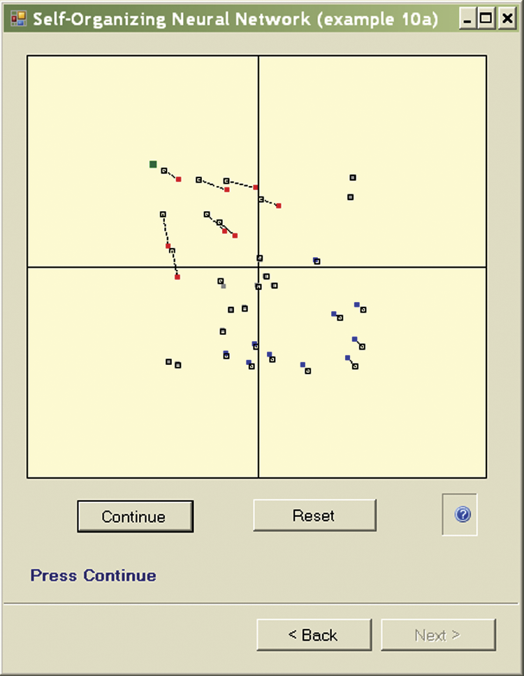
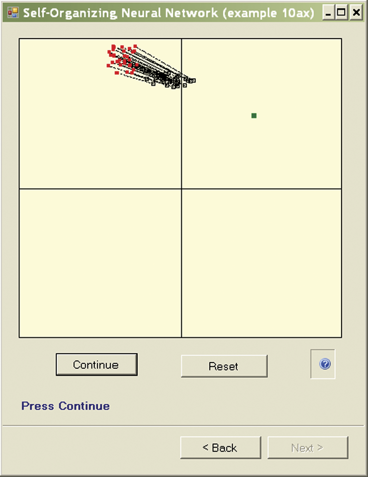
At the time of the emergence of a specific input signal of the learning set, it will appear on the screen as a green square much larger than the point of identifying the location of a neuron (Figure 9.5). After receiving the signal at input, all the neurons of a self-learning network define their output signals (based on the components of the input and its weights). These signals can be positive (red points indicating the neuron “likes” the object) or negative (blue points indicating the neuron “dislikes” the object). If the output signals of some neurons (both positive and negative) have low values, relevant points exhibit gray color (corresponding to indifference to the subject).
All the neurons of self-learning networks correct their weights based on the input signals and established output values. The behavior of each neuron during correction of its weights depends on the value of its output (response to stimulation). If the output neuron was strongly positive (red on the screen), the neuron weights will change toward the “likes” point. If the same point is presented again, the neuron will react even more enthusiastically; the output signal will have a larger positive value.
Neurons that show negative reaction to a pattern (blue points on the screen) will be repelled from it. Their weights will motivate them to even more negative responses to the pattern in the future. In Example 10a, you can see the “escape” of negatively oriented neurons outside the viewing points that represent them. In this case, the neuron is no longer displayed. This is a natural result if we consider that self-learning neural networks typically exhibit equally strong attractions and repulsions.
You can see clearly the moving of points showing the positions of the weight vectors of neurons because the program presents an image at each step to show the previous and new locations of points representing the neurons (Figure 9.6). Furthermore, the old location is combined with a new one by a dotted line so you can follow the paths of neurons during learning.
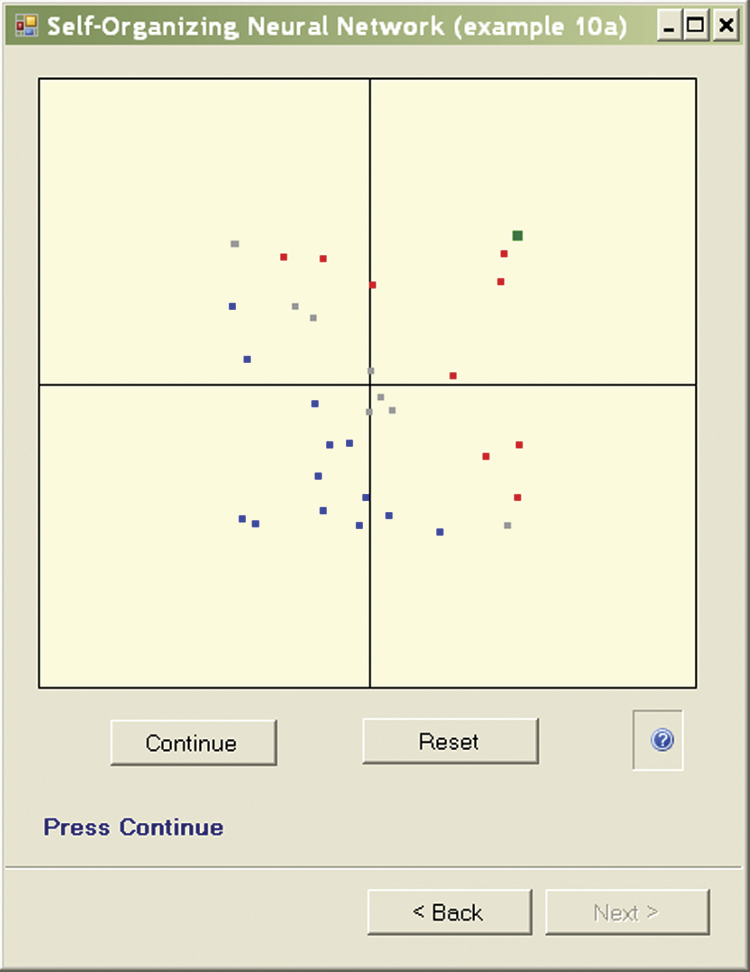
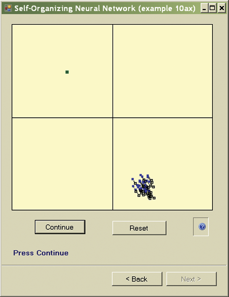
In the next step, the new neuron weights become old. After the system displays the next point step the cycle begins again (Figure 9.7) and a new object is presented to the network, perhaps belonging to a new class (Figure 9.8). If you repeat this process long enough, a cluster of neurons specialized in the recognition of typical objects belonging to a group will appear in each quadrant (Figure 9.9). In this way, the network specializes its recognition capabilities.
After you observe the processes of self-learning, you will certainly see that this learning strengthens the innate tendencies of neural networks expressed in the initial (random) spread of weighs vectors. These initial differences cause some neurons to respond positively to an input object while others react negatively. The correction of all neurons is made in such a way that they learn to recognize common elements appearing at the inputs and effectively improve their recognition abilities without interference from a teacher who may not even know how many objects should be recognized and what their characteristics are.
To ensure that self-learning proceeds efficiently, we must provide initial diversity in the neuron population. If the weight values are randomized in a way that ensures the needed diversity in the population, self-learning will proceed relatively easily and smoothly. If, however, all neurons will have similar “innate tendencies,” they will find it difficult to handle all emerging classes of objects and exhibit the phenomenon of “collective fascination,” which causes it to reactive positively to a selected object and ignore others.
The diversity in Example 10a was intentional. Because the initial random distribution of neurons is of primary importance we prepared a variant of the program called Example 10ax that allows a user to request random spreading of the features or draw the initial positions of the neurons from a narrow range. The field (checkbox) called Density must be set properly in the initial panel (left screen in Figure 9.10). Initially, it is better to choose widely spread neurons and not set a density value. After you are familiar with basic pattern of the network self-learning process and ready to see a new reaction, check the Density box.
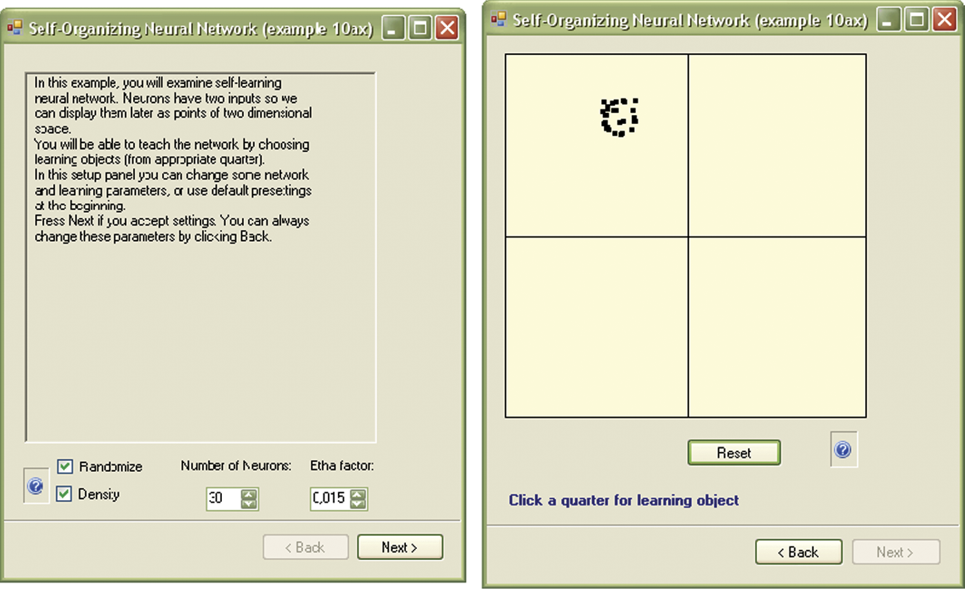
Initial window with parameters (left) showing effect of drawing initial values of weight vectors in Example 10ax program.
You can see how important the initial random scattering of neuron weights is. Figure 9.10, Figure 9.11, and Figure 9.12 show the results of insufficiently differentiating neuron weights.
You can use the Example 10a and Example 10ax programs to carry out a series of studies, for example, to examine the effects of a more “energetic” self-learning process by increasing the value of the learning rate (etha).
Other interesting phenomena can be observed by unchecking the Randomize default parameter. The network will always start with the same initial weight distribution and you can observe the effects of the order and frequency of presenting of objects from different quadrants on the final neuron distribution.
Another parameter for experimentation is changing the number of neurons (number of plotted points). This value can be reset by going back to the first window appearing after program launch (Figure 9.3 and Figure 9.10) and the results are interesting. The initial distribution of certain neurons can be considered by analogy to the innate process by which a human learns from his or her experiences.
9.2 Observation of Learning Processes
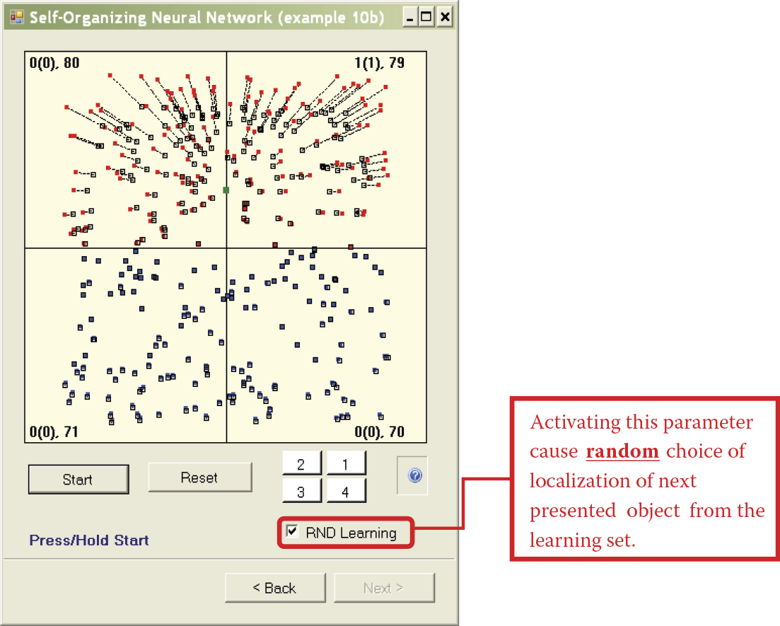
Example 10a demonstrated the machine learning process of a neural network. It required many presses of the Continue button to see results. To eliminate the repetitive use of the button, we devised Example 10b to implement the machine learning process almost automatically. As with previous programs, Example 10b starts by allowing a user to accept or change default values. You can then watch the process in the windows. The learning is “almost” automatic because you have an option via the Start button to observe the steps as learning proceeds. You can halt the operation to observe progress.
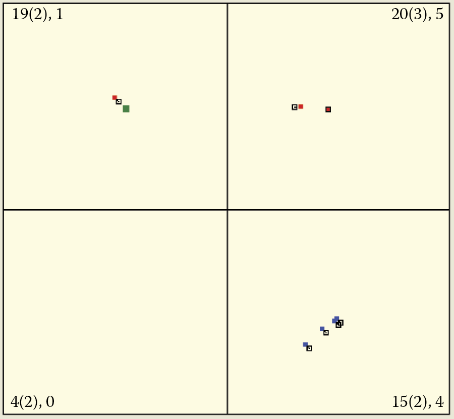
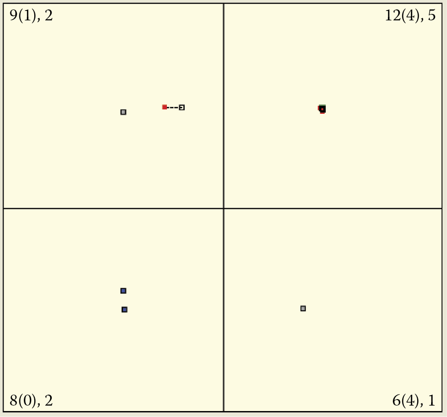
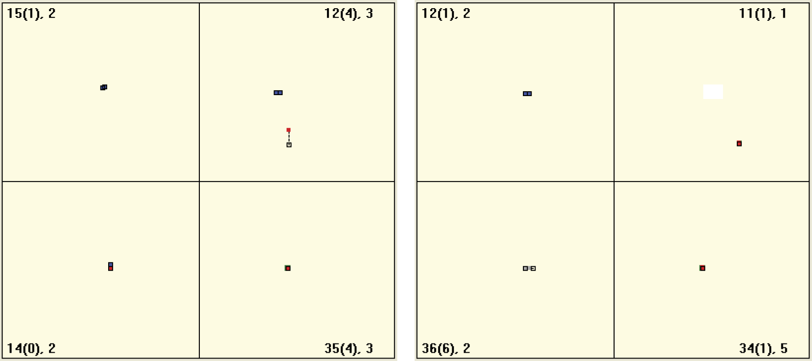
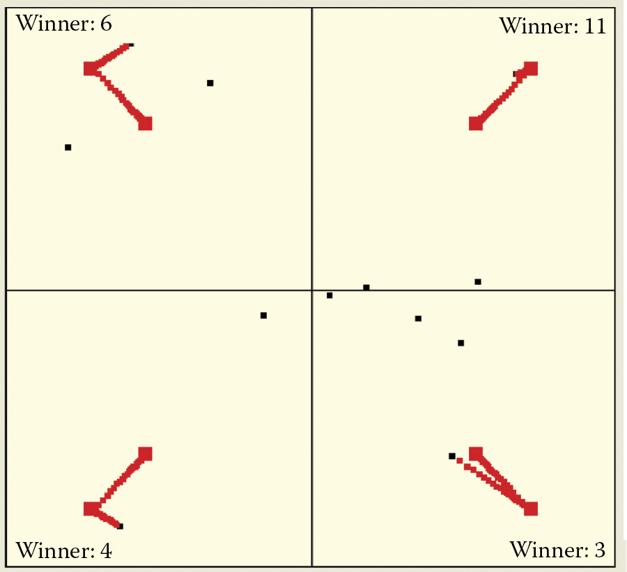
One issue to consider before starting the program in the mode described above is the network size. The program lets us simulate a network composed of freely chosen neurons, starting with a network that contains only a few neurons (Figure 9.13 and Figure 9.14). Because the network builds four clusters in four quadrants, there is no point in analyzing a network composed of fewer than four neurons, but you can see how a single neuron behaves. The simulation follows the program; the user monitors the process and draws conclusions.
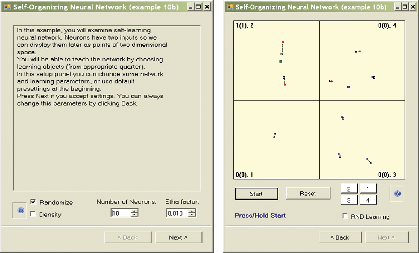
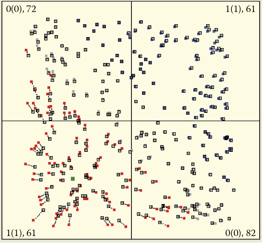
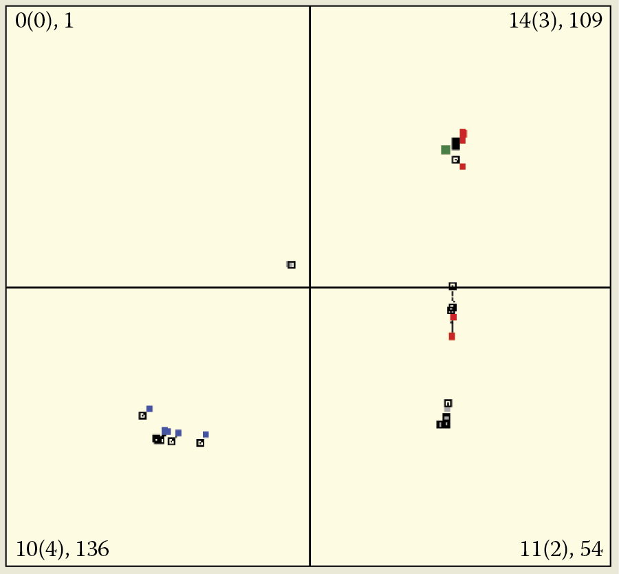
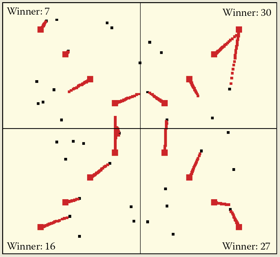
To make the observation of the ongoing processes easier, each quadrant displays additional information that indicates (1) how many times the object of a learning sequence was shown in the quadrant (this demonstrates the crucial role of initial presentations); (2) the results of the first nine presentations (in brackets); and (3) how many neurons are currently located in the quadrant. For example, the 10 (3), 1 notation in a quadrant means that the learning object appeared ten times, three times in the first nine presentations, and one neuron is now located in the quadrant.
This information is especially useful for a system containing many neurons. It allows a user to the track the number of neurons and where they are, and interpret situations such as neurons that overlap near the repetitive point of a learning sequence object and make judgment difficult. Observing randomly appearing asymmetric effects caused when objects from a certain quadrant are presented more often than others is also an interesting exercise.
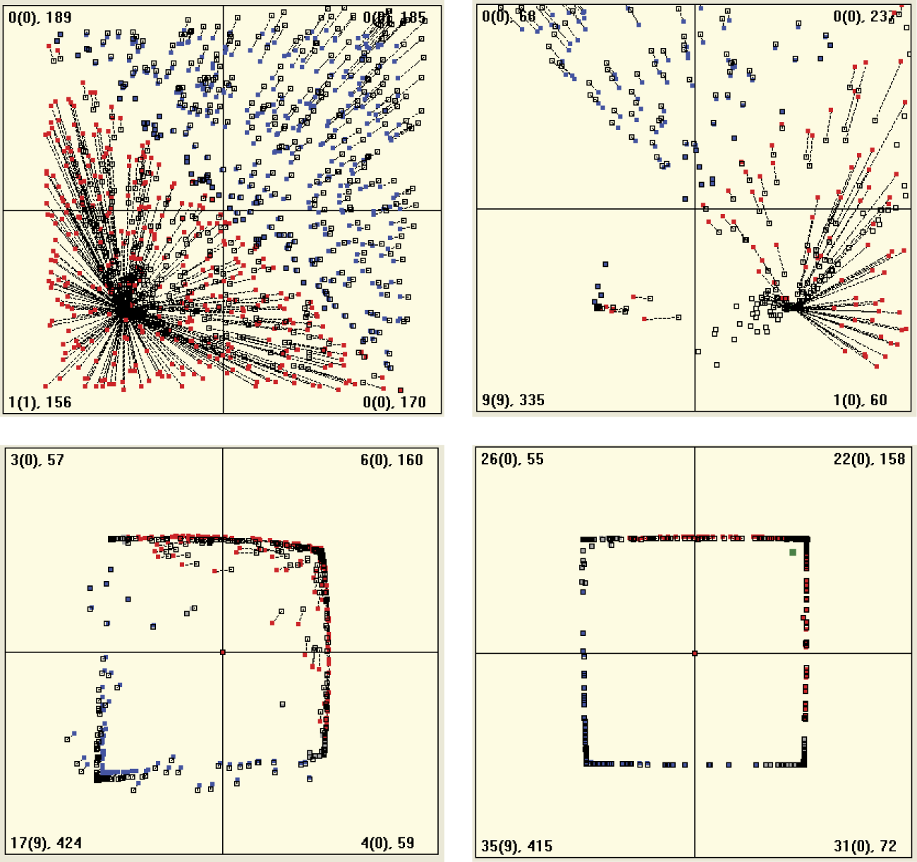
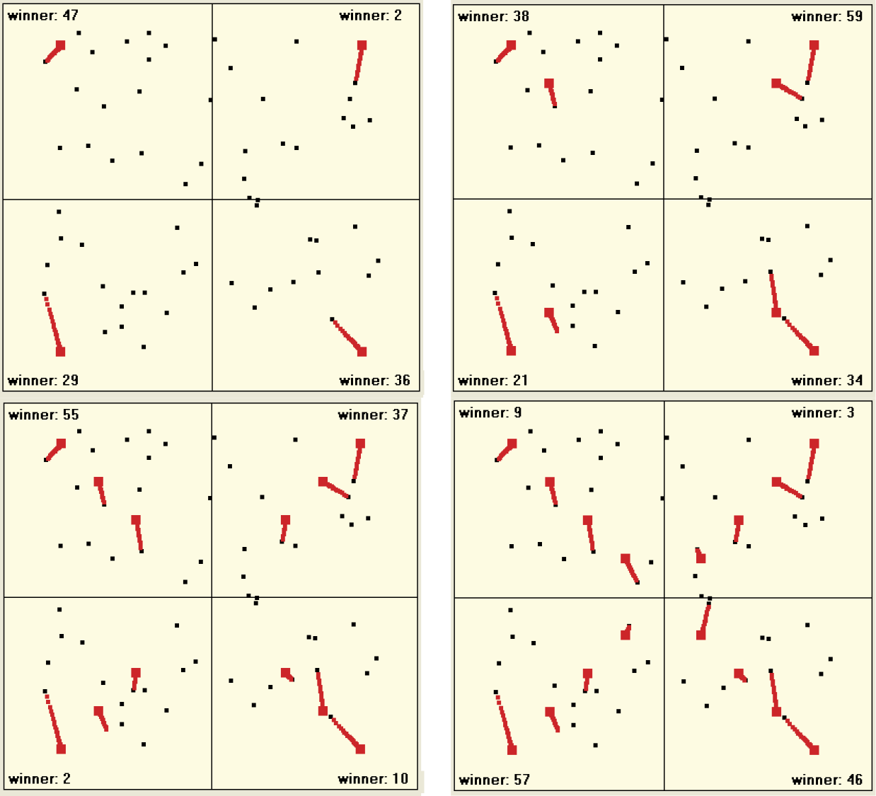
This program helps you understand how large networks, composed of thousands of neurons behave. Figure 9.15 and Figure 9.16 demonstrate how 700 neurons learn simultaneously. The program generates initial weight distributions for all the neurons and then shows input signal patterns as points in the centers of certain randomly chosen quadrants. Each input is followed by a vector weight change caused by the machine learning process. The next input object is shown and the next step of machine learning follows.
At first, when you click and release the Start button, machine learning proceeds step by step. It stops after every presentation of inputs so that you can view what happens in the network. The interruptions are eliminated later, and machine learning continues automatically and continuously. To simplify your view of more of the more complex operations of the system, subsequent figures in this chapter will display only the main parts of windows depicting point distributions for specific experiments.
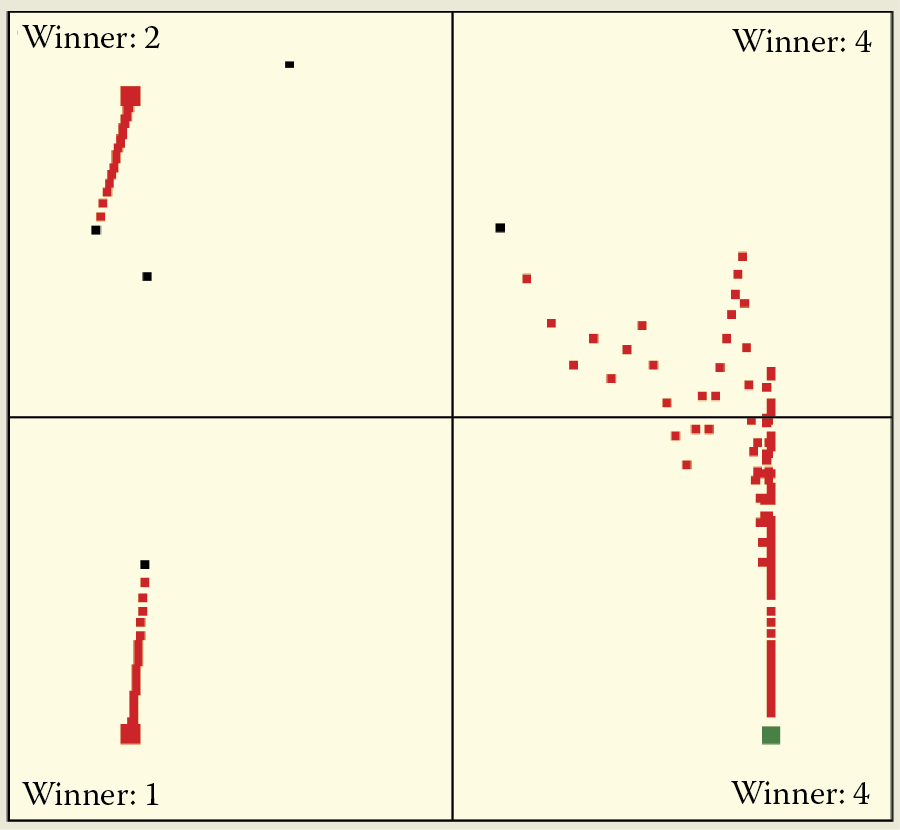
Machine learning processes and supervised learning can be achieved with different values of learning coefficients. Figure 9.15 shows how a network with a very high learning coefficient behaves. It displays an exceptionally enthusiastic attitude; every new idea attracts its attention entirely. The attracting object interests an enormous number of neurons that want to recognize and locate the object as quickly as possible. The attractor tactic enables a network to learn quickly but also causes immediate saturation of its cognitive potential. A minor number of attractors (in comparison with the number of neurons) can completely involve all the neurons in attempts to recognize them. As a result, the neurons will have no adaptation capabilities left for recognizing new patterns and thus the network becomes unable to accept and assimilate new ideas.
A network with small consolidation coefficients behaves differently. When a new object appears, the network reaction is calm and balanced (Figure 9.17). This is why learning is not a fast process. Compare Figure 9.18 depicting a similar learning level of a “calm” network and Figure 9.16 that displays an “enthusiastic” network. The network retains a reservoir of neurons that are not yet specialized and are thus able to accept and assimilate new signal patterns.
Slow and deliberate beginning of machine learning process in system with low value of learning coefficient (etha).
Similar stage of machine learning process shown in Figure 9.14 . We see numerous “vacant” neurons with low values of learning coefficients.
The acceptance of new ideas by some humans is similar. Some people accept an idea uncritically at first (e.g., a political issue). They learn about it, identify with it, and then become fanatic to the point where they cannot accept other ideas or views, almost as if their brains have no space left. In extreme cases, their religious or political ideas possess them to the point where they are capable of murdering and torturing those who oppose their views.
Researching a highly excitable neural network may produce an interesting phenomenon. If a “fanatic” network receives no signals from its attractor for a long enough time, it will rapidly change its focus. All the points previously associated with a certain pattern (or fanatic idea) will suddenly migrate toward (and fixate on) a completely different pattern (Figure 9.19). Humans behave similarly. The literature is full of examples of people who suddenly changed their beliefs or lurched from one extreme to another.
Left: Attraction of all neurons to objects coming from one class only. Right: Abandonment of attractor and transfer of recognition of all neurons to second attractor.
The phenomena described above occur only in networks with high learning coefficient values. Shifts that can be seen in Figure 9.18 and Figure 9.19 arise when the learning sequence objects belonging to the same class are not identical and a network learns continuously.
A network model with a low learning coefficient (Figure 9.17) resembles a reluctant human who has to examine every new idea completely before assimilating it on a limited basis. However, once this human adopts a preference, he or she generally does not change it easily.
9.3 Evaluating Progress of Self-Teaching
We will now present some simple experiments you can conduct to analyze the features of the program described above. These experiments will help you to learn more about the characteristics of the self-teaching processes in neural networks and the impacts of changes on learning progress. We will describe the use of the Example 10b program which is designed so that you can work with it and discover the various features it presents.
After activating learning with a given number of neurons, we can observe how the neurons detect repetitive presentations of certain characteristic objects within the input data. You will notice immediately that the initially chaotic set of points representing the locations of neuron weights display an inclination to divide the population of neurons into as many subgroups as the number of object classes appearing at the input.
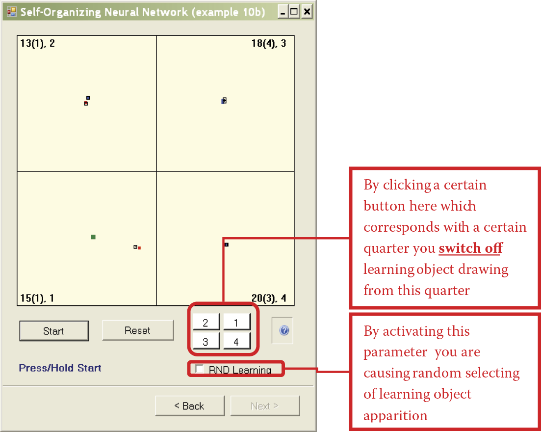
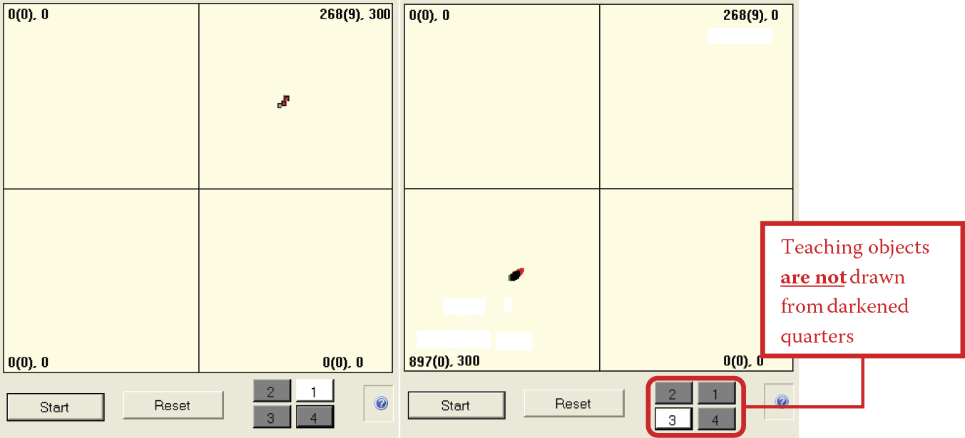
This is easy to check. During a simulation, when you click on the picture with a number of a quadrant (1 to 4), the objects appearing during teaching will only come from three or fewer quadrants, not all four. Objects from the chosen quadrant will be omitted and the quadrant will be marked with a darker color. This option of the program allows you to assess the efficiency of detection performed by the network and the number and types of object classes it should recognize (Figure 9.20 and Figure 9.21).
Beginning of self-teaching process during which objects from second quadrant are omitted.
Final stage of self-teaching process during which objects from second quadrant are omitted.
At the beginning of the teaching process, the network partially organizes neurons that potentially may recognize the objects of the missing class (Figure 9.21), leading to increased focus of the network on these objects. However, even at the final stage of the self-teaching process, when the network already achieved a high level of recognition and identification of objects through self-teaching (three clusters in Figure 9.21), the area with no attractors still contains spare neurons. They are dispersed randomly and they will disappear as the self-teaching process continues.
Sometimes, even after basic learning has ended and a new object appears, the neurons take over the learning process rapidly and attempt to identify the new object. Even after a long period of systematic self-teaching and considerable experience, a network may deploy all its neurons into a certain orbit of an attractor. If a new object appears after this type of network petrification, it will have no free neurons capable of accepting the new object and learning to identify it. Thus, a long process of self-teaching leads to the network’s inability to accept and adapt to new inputs.
Humans are subject to the same phenomenon. Young people adapt to new conditions and acquire new skills (e.g., using computers) easily. Older people who have experience performing certain functions and recognizing situations may take a skeptical view of new ideas and resist learning new tasks.
The detailed course of self-learning depends on the initial set of the values of neural weights—the innate qualities of individuals. Learning also depends on the sequence in which the learning series objects (life experiences) are presented. Some people retain their youthful curiosity and sense of amazement, and approach new situations enthusiastically. Others remain rigid and cling to their biases. You can track this process in a network.
Example 10b is constructed so that pressing the Reset button will restart the self-teaching process with the same number of neurons, randomly chosen initial weight vector values, and a new and random set of learning objects assigned to chosen quadrants. By clicking on the buttons that mark the quadrants, you can freely switch presentations of objects on and off. In essence, this allows the user full control of the experiment.
If you repeat the learning process, you will see that the tendency for self-organization—the spontaneous tendencies of individual neurons to identify certain classes of input signals—is a constant feature of a self-teaching neural network. It does not depend on the number of classes, the number of neurons, or the arrangement of their initial values of weights. You will also notice that “more talented” networks consisting of more neurons can accept new types of inputs and maintain new skills for longer times.
9.4 Neuron Responses to Self-Teaching
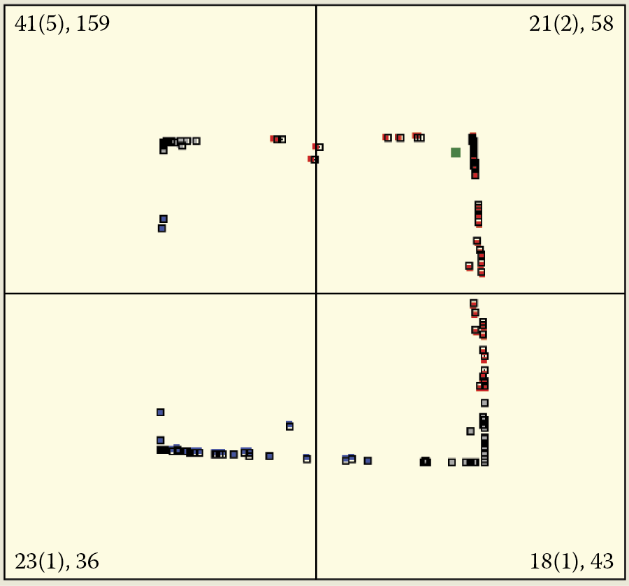
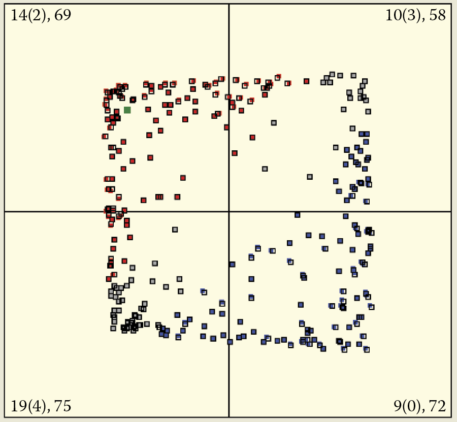
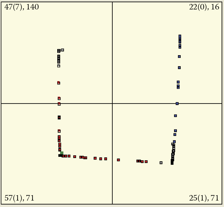
You can perform various analyses using Example 10b. We suggest you begin with an analysis of the influence of object presentation on self-teaching. The program has no built-in mechanisms that present the relevant facts “on a plate.” However, if you watch the simulated self-teaching process several times, you will notice that the classes whose objects are shown more often attract far more neurons than the classes whose objects appear less frequently (see Figure 9.22 results for first and second quadrants). This may lead to a lack of willing neurons’ recognition of some classes of inputs, especially in networks with small numbers of neurons (compare third quadrant in Figure 9.22).
This is a big problem that was mentioned briefly in an earlier chapter. As a result of this tendency of neurons to focus on certain inputs, self-teaching networks must contain many more neurons than networks that carry out the same tasks after training by a teacher.
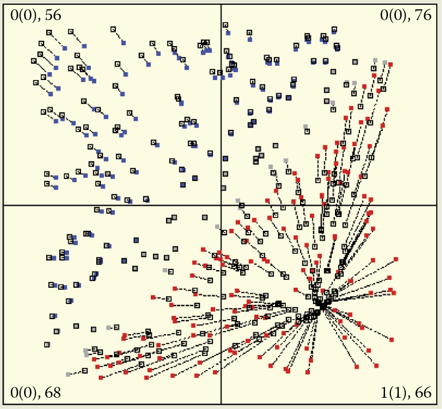
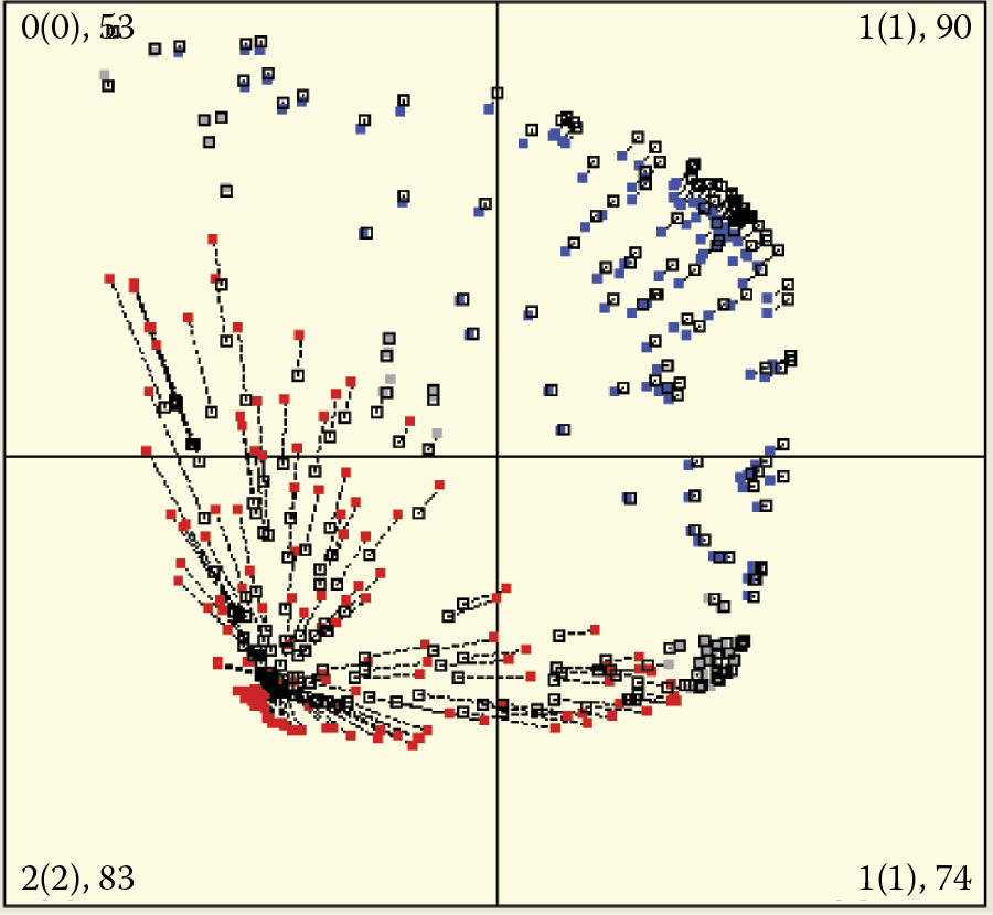
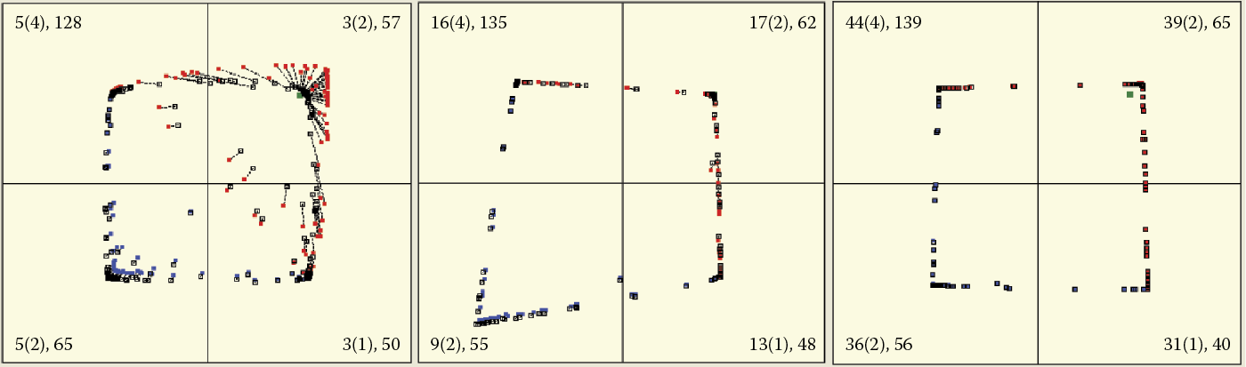
Examining the self-teaching process on many samples will demonstrate that the first reaction of a network is particularly relevant. This can be seen in Figure 9.23. The reproduced images of the first (top left) and final (bottom right) self-teaching steps accidentally draws only objects of the third quadrant in the first nine steps of the algorithm. Notice how it strongly affected the final distribution of the number of neurons in different quadrants.
Note that the overwhelming influence of experiences on later development of preferences and habits can also be seen in humans. If certain reactions (quadrants) are initially disabled (e.g., by an unhappy childhood experience), the representation of the initial experiences (represented in the model by a quadrant containing signals) remain visible in the network as limited or absent signals. This observation explains why successes in eliminating the effects of a difficult childhood are so rare.
Observing the attraction processes of some neurons and repulsion reactions of others allows you to imagine what happens when your brain encounters new situations and must analyze them. Consider a neural network with a large number of neurons. Figure 9.23 shows the self-teaching process of a network containing 700 neurons. You will see the mass movement of the “states of consciousness” as many neurons converge toward the points corresponding to the observed input stimuli and thus become detectors of these classes of input signals.
You can also view the “revolution” that takes place in the first steps of the self-teaching process. This is best done by conducting an experiment in steps. Information about which objects are often and rarely shown in the initial stages of learning is shown as numbers in the relevant quadrants, so you can easily observe and analyze the basic relationship between the frequency of presentation of the specified object in the training data and the number of neurons ready to recognize them. You can observe the effect especially clearly when you compare the results of many simulations. Recall that the results of all the individual simulations strongly influence the initial distribution of the weighting factors of individual neurons and the order of presentation of the training set objects. Both these factors are randomly drawn in the experimental programs.
9.5 Imagination and Improvisation
After you observe how networks form and classify ideas, you can move on to more subtle network activities. You may have noticed when practicing examples with large number of neurons the process of formation of neuron clusters recognizing main objects introduced to the system. We can also view tracks of neurons. These neurons are spontaneously aspiring to detect and recognize inputs and related objects (Figure 9.24). During self-learning, these neurons act as detectors focused on signaling the presence of real-life objects but “fantasize” about non-existing entities with astounding regularity.
Parameter localization for neurons (detectors of hybrids) ready to detect objects having properties shared by real objects.
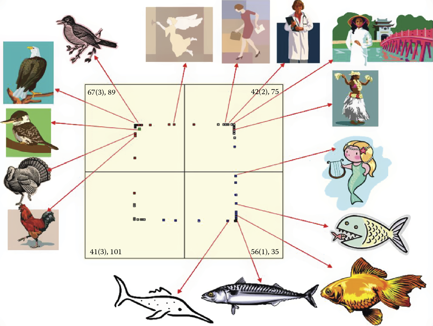
How does this impact results? A network that is shown a fish and a woman repeatedly will learn to recognize both images but this requires explanation. At appropriate points, some neurons will correctly recognize a woman and a fish; some will be ready to recognize entities displaying the features of the fish (tail) and the woman (the head and shoulders). Although the creatures were not shown during the self-learning process, the network prepared neurons to detect them. In a certain sense, the network may have “imagined” them.
Following a similar principle, the same network that developed an ability to recognize bird species can associate bird features with the characteristics of a woman (head, hands, dress) and thus create an image of an angel (Figure 9.25).
After repeating many experiments, we are convinced that every young (not fully taught) neural network will have a tendency to invent objects that do not exist. If experiments regularly prove that women and fish both exist and no creatures share the properties of women and fish (e.g., mermaids), the neurons will change their specialization to accommodate the hybrid combination.
These neurons will proceed to recognize real-life creatures instead of fantasies. They exhibit this tendency during experiments. If a hybrid creature (e.g., a bat that is in essence a mouse with wings) is presented, a network’s previous experience with combination objects will facilitate the detection and classification tasks.
It appears that this ability to invent non-existent objects by combining elements of impressions and experiences is displayed by networks only during the early stage of self-learning. The analogous human behavior is a child’s enjoyment of fairy tales and legends that are boring to adults. When you observe feeble chains of neurons emerging during self-learning, as shown in Figure 9.26, then you may be watching the formation of associations, analogies, and metaphors.
During some experiments, certain (usually single) neurons remain outside the areas concentrated near the spots where input objects appear. Actually, these are of little practical significance because most neurons are taught easily and are subject to precise specialization. The majority of them aim toward perfection in handling detection and signaling of real-world objects. The neurons that are out of touch with reality will stay and retain (Figure 9.27) their images of non-existent entities.
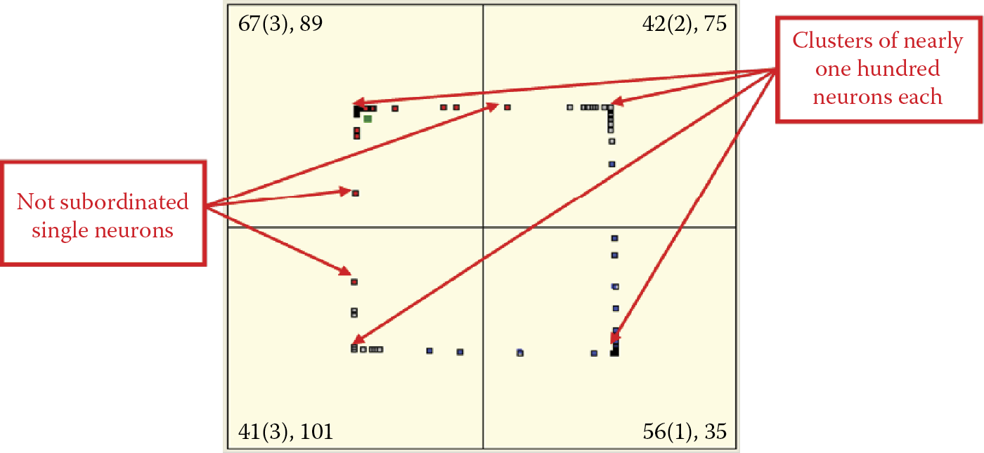
Appearance of single neurons outside global centers during advanced self-learning (after 200 steps).
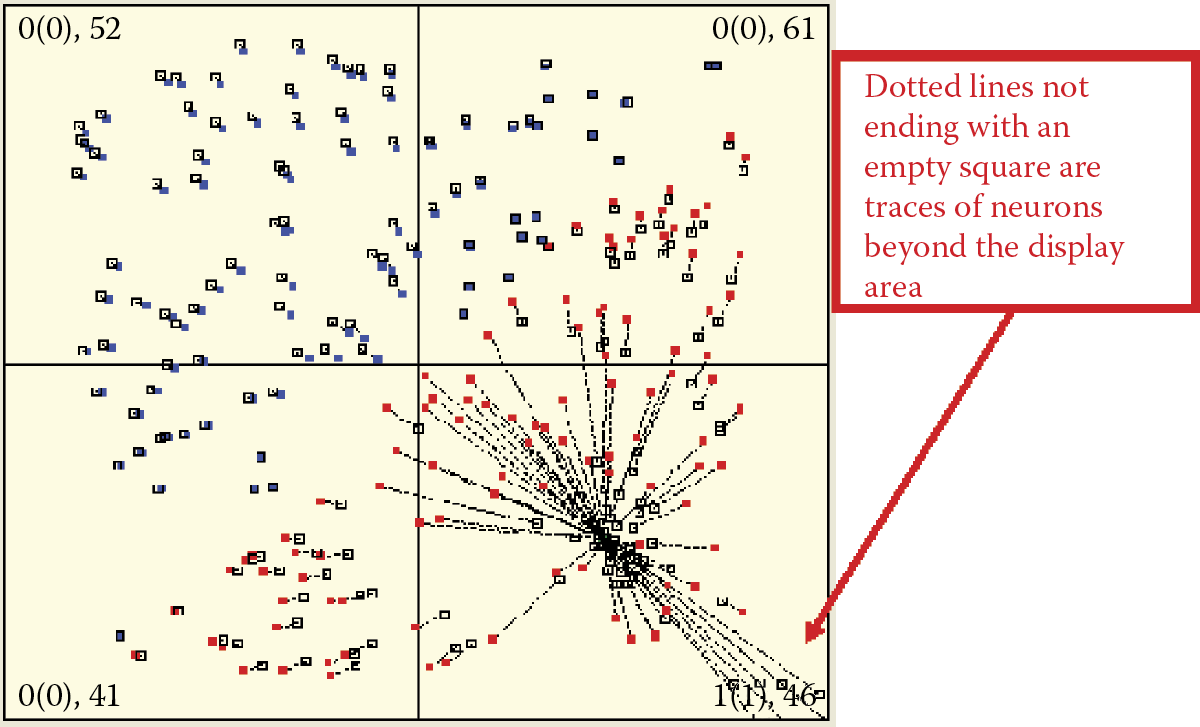
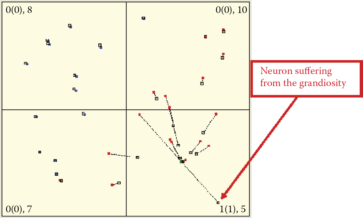
If you watch carefully the initial stages of self-learning, you may notice another interesting phenomenon. After an object is shown at a certain point in the space of the input signals, a few neurons will change their original positions. When they reach a new location distant from the original one, they remain in the same direction as the input object even though they are far from the origins of the coordinate system. This is a rare event because it depends on the initial distribution of weight coefficients. If you patiently repeat your experiments, you will notice this change (Figure 9.28). As a rule, rebellious neurons land outside the borders of the limiting frame and they can be seen because lines with no empty squares at the ends will appear.
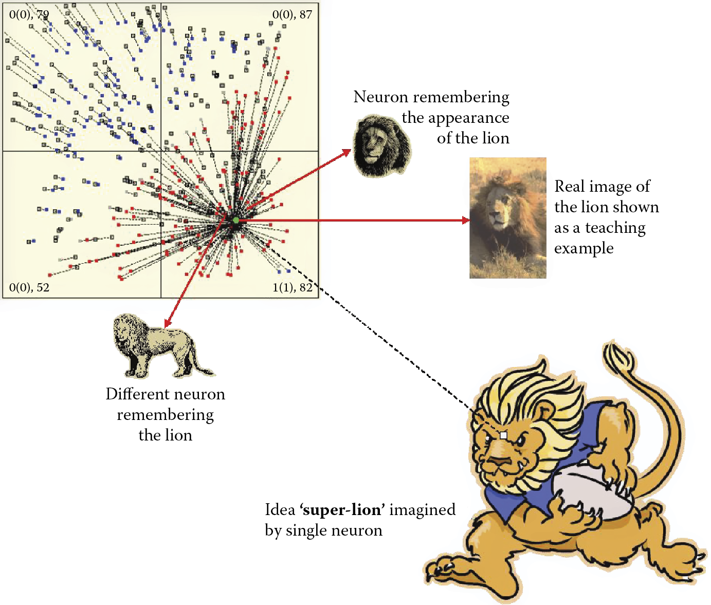
Neurons that wander far at the start of self-learning will be pulled back in consecutive stages of teaching to the area associated with the presented standard and they will find their way back to where they should be. We are concerned with them because they illustrate a well-known psychological effect known as grandiosity (Figure 9.29). Indeed, a neural Gulliver escaping the display area becomes the standard of an object that displays roughly the same features as the model object perceived at the start of teaching—with all its features magnified.
If a lion is shown, the image produced after enlarging its perceivable features depicts a real monster that has huge fangs and claws, ruffled mane, and dangerous roar. The image contains all the features of a lion, only larger, as in Figure 9.30. Such exaggerated ideas of a neural network are usually short lived and the system behaves as programmed.
At the end of self-learning, most neurons form tight clusters near the spots where input objects will signal (they have already chosen a master and are ready to serve). Sometimes, rebellious points appear beyond the display area. Despite their resistance, they are pulled back to the areas where real objects are recognizable (Figure 9.31). These neurons pursue different paths and the results may be incorrect reactions. As time passes, the rebel neurons are forced to join the conforming majority on the correct path. On occasion, an unexpected input gives these non-conformists a chance to win, but such occasions are rare.
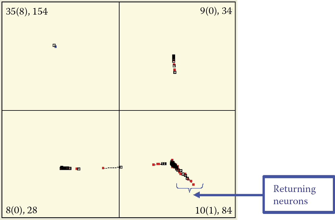
Pulling back neurons that escape in the initial stage of teaching and create fictional representations of data—effect known as grandiosity.
9.6 Remembering and Forgetting
This chapter concentrates on the activities of self-learning networks such as storing information and gaining knowledge, and explains how they accomplish these tasks. Networks are also subject to another event that occurs daily in human life: forgetting. This phenomenon is burdensome in some situations, but it is an essential biological function. Our living environments change constantly. Actions we mastered at some stage of life may become outdated or even harmful, and we are compelled to gain new skills and forget earlier ones. Forgetting unneeded information prevents conflict and confusion.
We can use neural network simulation to observe and analyze this process. New objects appearing during simulation of self-learning networks may divert neurons from tasks they already learned. In extreme cases, new objects can “kidnap” neurons that recognize earlier patterns that are obsolete (Figure 9.32). In this situation, the neural network recognizes quite well all four patterns that were presented to it. Please note that pattern number 1 has the strongest representation in the 1st quarter.
First stage of forgetting process during self-learning. Network still possesses earlier (class 1) knowledge.
The network in the figure recognizes all four patterns presented to it. The first pattern in the first quadrant displays the strongest representation. At this point, self-learning is interrupted intentionally and the experiment proceeds to “kidnapping.” A class is a collection of objects that are similar to each other within a class and different from the objects belonging to other classes—each object is an instance of its class. Classes can be named (e.g., “dogs,” “cats,” “horses,” “cows”), but in our considerations the names are not important. Therefore, we use numbers instead of names. Our discussion is concentrated on classes 1 and 4, because class 1 loses neurons and class 4 gets them. Classes 2 and 3 are stable, and therefore not interesting. Neurons recognizing objects of class 1 change their specializations immediately. They quickly focus on recognizing other classes of objects (class 4; Figure 9.33 left). The earlier familiar class is forgotten but not completely. Even extended learning courses leave traces of earlier learning in neuron memories (Figure 9.33 right). Although the trace in the figure is very weak (involving only one neuron), it significantly altered the position of the neuron.
Forgetting of class 1 when trace in memory is not enforced systematically during self-learning.
Humans have similar experiences. You may be interested in botany and learn the names of and characteristics of new plants. If you fail to revise and solidify your knowledge quickly, you will forget what you learned. The old information will be blurred by new knowledge and plant identification will be difficult.
9.7 Self-Learning Triggers
During experiments with Example 10b, we saw that the impulsive nature of self-learning caused some classes of objects to be stronger (better recognized) and other classes to be weak or absent. This is an important shortcoming of self-learning methods and we will describe it in detail in Section 9.8.
We should demonstrate that self-organization and self-learning occur only when a network is based on patterns in the input data sequence. The situation in Example 10b was simple. The objects shown to the network belonged to a specific number (usually four) of well-defined classes. Furthermore, the classes occupied distinct areas, namely the central parts of four quadrants of the system.
The objects appeared in a random sequence but were not located in random places. Each time a point presented to the network was located (with some deviation) in the central area of a given quadrant, it represented an example of an object. A completely typical (ideal) object would have appeared exactly in the center of the quadrant. This type of object representation may reveal a familiar result. The self-learning process caused neurons to form groups specialized to recognize specific patterns: combinations of slightly varied object representations from one class—variations of the same perfect pattern.
We now consider how a network behaves when points used during learning are located completely randomly. In an example from an earlier chapter, we discussed a space probe sent to Mars. In this example, no Martians are found. The landing vehicle sensors receive images only of random shapes of Martian dust formed by winds.
A feature of Example 10b allows easy observation of this situation during learning by activating the RND learning option. You must check the box because this option is disabled by default. From this point, you will not see the quadrant in which the learning sample is located (Figure 9.34). It is not important if you enable random point selection from all quadrants as in the figure. The sample object will appear randomly anywhere in the coordinate system.
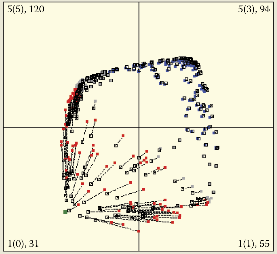
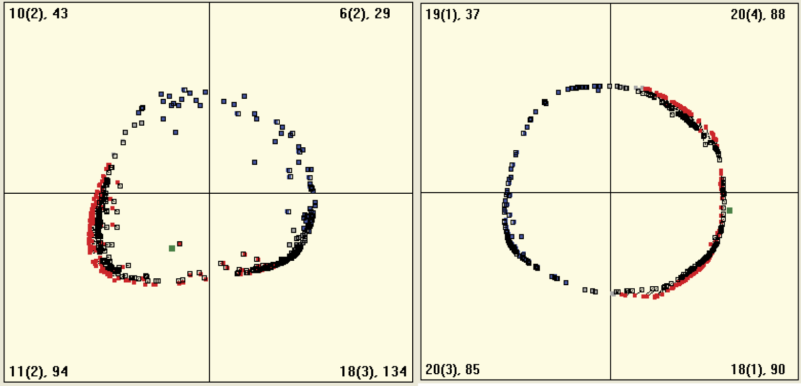
Because of the lack of order, no information will be generated in the input data sequence. Neurons may be attracted to the center of the area on one occasion and at other times will be pushed outside (Figure 9.35). In this case, the self-learning process will not lead to the creation of visible groups of neurons. Instead the neurons will form a large circle within which the mean signal pattern will appear. When you watch this aspect of self-learning for a time, you will see that the size and location of the circle change with every presentation of the learning sample (Figure 9.36). However, no groups of neurons will emerge because the input data contain no such groupings.
The conclusion is both optimistic and pessimistic. The optimistic view is that the self-learning of a neural network may help it find unknown patterns present in the input data; users do not have to know what and how many patterns are present. Sometimes, self-learning networks appear to answer unasked questions. In general, they accumulate knowledge during learning and also discover it. This is an awesome development because computer science has many good tools (Internet and databases) that yield good answers to good questions. We can even obtain good answers to stupid questions but no commonly available tools can find answers to unasked questions.
Self-learning neural networks have such abilities. Finding answers to unasked questions is called data mining. It is used, for example, to determine customer behaviors and preferences of mobile phone users. The marketing specialists can make use of even the smallest piece of data about repeatable and common customer behaviors. The result is a huge demand for systems that provide such information.
The (slightly) pessimistic part relates to a self-learning network that generates data devoid of useful information. For example, if input values are completely random (without explicit or implicit meaning) even the longest learning process will not provide meaningful results. This characteristic has a positive side. Neural networks will never replace humans by generating new ideas suddenly and spontaneously.
9.8 Benefits from Competition
Any type of neural network can be self-learned. The most interesting results arise by enriching self-learning with competition. The competition between neurons is not a new concept; it was described in Section 4.8. Example 02 demonstrated the operations of networks in which neurons compete.
All neurons in competitive network receive input signals (generally the same signals because the networks are usually single-layer types). The neurons then calculate the sums of those signals (multiplied by weights that vary with each neuron). All values calculated by neurons are compared and the “winner”—the neuron that generated the strongest output for the input—is determined.
The higher the output value, the better the agreement between the input signal and the internal pattern of a neuron. Therefore, if you know the weights of the neurons, you can predict which ones will win by presenting samples that lie in particular areas of the input signal space. The prediction is easy to make because only the neuron whose internal knowledge is in accord with the current input signal will win the competition and only its output signal will be sent to the network output. Outputs of all the other neurons will be ignored.
Of course, the success of the neuron is short-lived. The arrival of new input data means another neuron will win the competition. This is not surprising there. The map showing the arrangement of the weight values determines which neuron will be the winner for any given input signal—the neuron whose weight value vector is the most similar to the vector representing the input signal.
A few consequences surround the winning of a competition by a neuron. First, in most networks of this type, only one neuron has a non-zero output signal (usually its value is 1). The output signals of all other neurons are zeroed. This is the winner-takes-all (WTA) rule. Furthermore, the self-learning process usually concerns only the winner. Its (and only its) weight values are altered so that presentation of the same input signal will cause the same winning neuron to produce even output. Why is that?
To answer, let us examine carefully what exactly happens in a self-learning network with competition. At the start, we present an object represented by its input signals. The signals are propagated to all neurons and form a combined stimulation. In the simplest case, combined stimulation is a sum of input signal multiplied by the weight values. We can apply the same rule to neurons with nonlinear characteristics. The more weight values of the neuron are similar to the input signal, the stronger the combined stimulation of neuron’s output.
We already know that the sets of weight values can be treated as input signal patterns to which each neuron is particularly sensitive. Therefore, the more the input signal is similar to the pattern stored in the neuron, the stronger the output when this signal is used as an input. Thus, when one of the neurons becomes the winner, its internal pattern is the most similar to the input signal among signals of all the other neurons. But why is it similar?
In the beginning, this result may arise from random weight value initialization. The initial values of these are random in all networks. The randomly assigned values are more or less similar to the input signals used during learning process. Some neurons accidentally acquire an innate bias toward recognition of some objects and aversion to others. The learning process later forces internal patterns to become more similar to some kinds of objects at each step. The randomness disappears and neurons specialize in the recognition of particular classes of objects.
At this stage, a neuron that won by recognizing the letter A will probably win again when another A is presented on an input even if it is slightly different from the previous sample. We always start with randomness. Neurons decide which of them should recognize A, which should recognize B, and which should signal that a character is a fingerprint and not a letter. Self-learning process only reinforces and polishes a neuron’s natural bias (again randomly assigned during initial value generation).
This happens in every self-learning network, so what does competition mean? Competition makes self-learning more effective and efficient. Because initial values of weights are random, a few neurons may be biased toward a single class of object. Without competition, the bias will be strengthened simultaneously in all the affected neurons. Eventually there will be no variety in behaviors of neurons. Neuron behaviors will become more similar as shown in experiments with Example 10b.
When we introduce competition, the situation changes completely. Some neurons will operate more suitably for recognizing the input object than their competitors will. The natural consequence is that a neuron whose weight values are (accidentally) most similar to the presented object will become the winner. If this neuron (and only this one) is learning during this step, its inborn bias will develop further. The competition will stay behind and compete only for recognizing other classes of objects.
You can observe self-learning with competition using the Example 10c. We designed competitive learning in a task similar to the Martian family examples from Section 9.1. This time, the learning principle is different because the system will process completely new behaviors.
After starting, the application will display a parameter window. You can specify the number of neurons in the network. We suggest you manipulate only this parameter at first. It will be too easy to stray from the goal if you change several parameters.
The rule to determine the number of neurons is simple: the fewer neurons (e.g., 30), the more spectacular the results of self-learning with competition. You can observe easily that all neurons except the winner remain still; only the winner is learning. The exercise allows a user to trace changes of locations of learning neurons to reveal their trajectories. In Example 10c, a neuron that reaches its final location appears as a big red square that indicates completion of learning process for the particular class (Figure 9.37).
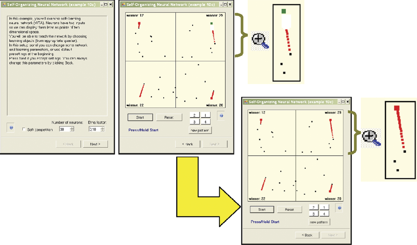
Example 10c parameter window and self-learning visualization in network with competition before and after eventual success.
When self-learning starts, you will see that only one neuron will be attracted to each point where objects belonging to a particular class appear. This neuron will eventually become a perfect detector for objects that belong to this class. You will see a big red square in a place where objects of that class typically appear during learning. If you click the Start button again, you will activate a step-by-step feature (if you hold the Start button down, the self-learning process will become automatic).
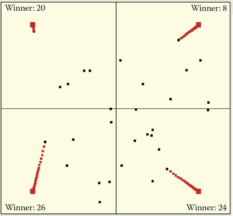
You can observe trajectories of moving weight vectors of specific neurons and read messages shown in each quadrant to see which neuron wins in each step. One neuron in each quadrant is chosen to win every time samples from the quadrant are presented. Moreover, only this neuron changes its location and moves toward a presented pattern. Eventually it reaches its final location and stops moving (Figure 9.38).
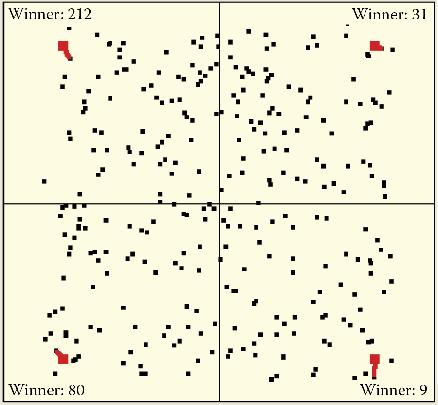
Self-learning with competition is more difficult to observe in systems with huge numbers of neurons. Unlike the classic self-learning process in large complex networks, learning with competition has a very local character (Figure 9.39). With many neurons, the distance from the nearest neighbor to the winning one is very short and therefore the trajectory of the winner is barely visible.
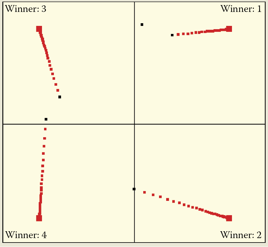
Conversely, with a small number of neurons (e.g., five), trajectories are long and spectacular. Moreover, the competition feature allows detection of even very weak initial biases toward recognizing some classes of objects can be detected. The biases will be strengthened during learning provided that competitors have even weaker biases toward recognizing objects of a particular class (Figure 9.40). The visibility of the sequence of changing locations will allow you to notice another interesting characteristic of neural networks: the fastest learning and greatest location changes occur at the beginning of the learning process.
9.9 Results of Self-Learning with Competition
Example 10c permits you to active the soft competition parameter (Figure 9.37 left). We suggest you use the default setting at first. We will experiment with soft competition after you understand the benefits and disadvantages of hard competition.
The hard competition displayed in Example 10c allows us to avoid cliques of neurons that have exactly the same preferences as those formed during our work with Examples 10a and 10b. If you are lucky, especially when working with networks consisting of many more neurons than classes of recognized objects, you may also avoid holes and dead fields in representations of input objects. Holes and dead fields denote the objects that no neurons could recognize. There is a high probability that when competition is used in a network, no neuron will be able to recognize multiple classes of objects. Conversely, no class of objects will not be recognized by any neuron, as noted in the old proverb that says, “Every Jack has his Jill.”
When learning with competition, the neurons other than the winner do not change their locations so they are ready to learn and accept other patterns. If objects from a completely new class suddenly appear during learning, some free neurons will be ready to learn from and identify this new class. Example 10c includes an option that allows you to order a new class of objects to appear.
To do that during simulation, click the New Pattern button. By clicking the button a few times, you can lead your network to recognize many more classes of objects than only four types of Martians. Learning with competition assigns each of those classes of input objects a private guardian neuron that from that moment will identify with this class (Figure 9.41). Usually some free neurons are available to learn new patterns that may appear in the future.
Unfortunately, the pure self-learning process combined with hard competition may cause abnormalities. When you initiate self-learning with a low number of neurons (four in the example application), one neuron will identify with and recognize one class of object. If new classes of objects are introduced when you click the New Pattern button, the “winner” may be a neuron that already specialized in recognizing some other class. Some class of input objects that gained a strong representation among neurons suddenly loses it. This is similar to the human reaction when new information replaces old information.
Figure 9.42 shows such an effect, in this case very strong. All trained neurons recognizing some objects re-learned after being shown new objects and started recognizing the new ones. This situation is not typical. Usually more neurons are available than recognized classes of objects are presented so the “kidnapping effect” is somewhat rare—it happens in one or two classes out of a dozen (Figure 9.43). That explains why some details disappear from our memories and are replaced by more intense memories. Unfortunately, memories that are “lost” may be important.
During experiments with Example 10c, you will notice other “kidnap-related” phenomena. New objects may kidnap neurons that already were in stable relationships with some class of objects and many neurons may still be free if they are distant. In the sample application, the phenomenon intensifies after one class of objects is shown and only when neurons start identifying with this group are new classes of objects shown. The new objects sometimes “steal” neurons from established classes. If all objects are shown at the same time, a competition can be observed when neurons are attracted to the first group and then to the second. You can see this in Example 10c when you start the self-learning process with a very low number of neurons; see Figure 9.44.
In this case, it is possible that a network will learn nothing despite a very long self-learning process. That will sound familiar to students who are not prepared to take a battery of examinations in mathematics, physics, geography, and history in a single day.
The solution may be “softening” the competition by clicking the Back button to return to the parameter window (Figure 9.37 left). Activate Soft competition by checking the box. From this moment, the application will apply softer limited competition. This means the winning neuron will be chosen only if the value of the output signal is exceptionally high.‡ Thus those neurons will be evenly divided between classes of recognized objects and no kidnapping of neurons that already belong to some other class will occur.
Unfortunately, you may see another worrying phenomenon. Under some circumstances (especially in networks with low numbers of neurons), no winner may appear among the neurons when an image is shown§ (Figure 9.45). Use Example 10c with soft competition to examine this phenomenon carefully. It will be easy, because the application uses special markers that show the locations of patterns of classes that are omitted (for which there is no winner among neurons).
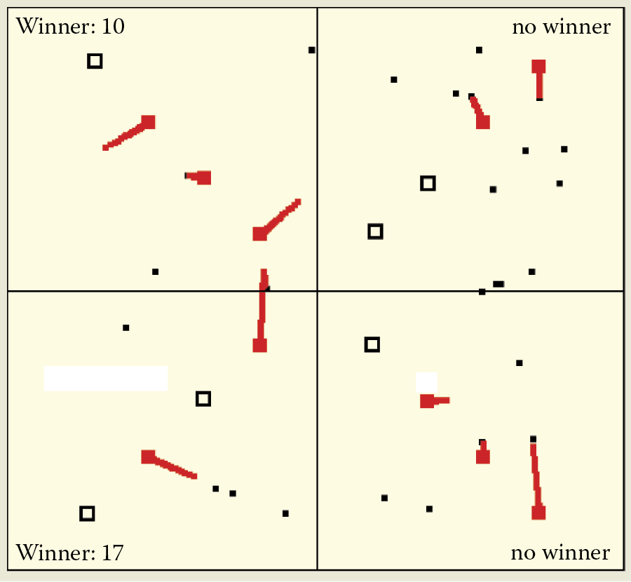
In the absence of strong competition, such omissions happen often, especially in networks with small numbers of neurons. In such cases for most classes in the network, voluntarily patterns will be created to allow automatic recognition of signals that belong to the specific classes. However, the “unlucky” class of signals no neuron wants to detect will have no specialized detectors. Such a neuron is like a person who has a flair for history, geography, and languages but cannot master mathematics.
Questions and Self-Study Tasks
1. Explain for whom, when, and why a self-learning neural network might be useful?
2. What determines whether points representing neurons in Example 10a will be blue or red?
3. Taking into consideration experiments described in this book and your own observations, formulate your own hypothesis on the influence that the inborn talents (represented by initial randomly organized weight vectors) exert on the gained knowledge represented by the self-learning process. Do you think that systems of small numbers neurons (such as primitive animals) are strongly influenced by their instincts and inborn qualities and more complex systems of many neurons (such as human brains) are more strongly influenced by external factors such as personal experiences and education? Find arguments for both views using self-learning networks of various sizes.
4. Describe the features of self-learning networks with very low and very high learning factor (etha) values. Do we observe similar phenomena in animal brains? When answering this question, remember that learning is easier for younger brains and it becomes more difficult with age (diminishing etha values in a neural network). For example, a young puppy has a brain that can be modeled by a network with a very high etha value. Its brain is different from the brain of an older dog (whose etha value may approach zero). Present the positive and negative views of this concept.
5. Do you think that a self-learning network that has “imagination” capabilities and can devise a new idea that has no similarity to known input signals used during self-learning?
6. Can you imagine a real-life situation that represents the experience described in Section 9.7? Explain what influence the situation would have for an animal brain or the brain of a young human.
7. Do you think that the forgetting mechanism triggered by over-learning described in Section 9.6 explains all the issues related to over-learning? Is the forgetting of information that is not constantly updated beneficial from a biological view or not?
8. Which adverse phenomena that occur during self-learning of a neural network can be eliminated by introducing competition? Which phenomena will remain?
9. In networks with competition, the winner-takes-all rule is sometimes replaced by the winner-takes-most rule. The Internet has information about this concept. What does the replacement indicate? What do you think?
10. Assume you want to design a self-learning network that can create patterns for eight classes. Prepare an experiment to determine how many more neurons (more than eight) the network should have at the start of self-learning, so no class will be omitted and the number of free neurons will be as low as possible.
11. Advanced exercise: Modify Example 10b to demonstrate how the etha parameter changes over time. Allow for the planned appearances of some objects during the network’s lifetime (e.g., early during learning or after training and experience). Run a series of experiments with such a real-life application. Describe your observations and develop conclusions. What observed phenomena have their representations in real-life situations? Which ones result from simplifying real neural networks (brains)?
12. Advanced exercise: Modify Example 10c to enable competition with a “conscience” (a neuron keeps winning but gradually lets other neurons win). Compare such a behavior with serious competition. What conclusions can you derive? Do those conclusions apply only to neural networks or could they also apply to real-life processes, for example in economics?
* The quadrant term for a space defined on the basis of a two-dimensional coordinate system is derived from mathematics. Although we promised that no mathematics details would be discussed, a little knowledge of coordinate systems is required for mastery of the material in this chapter. The signal space of a coordinate system is divided into quadrants (four sections). Assume the quadrants are numbered starting from upper right corner or quadrant (where variables on both axes are of positive value only) is numbered 1. The numbering proceeds counter-clockwise for consecutive quadrants. Quadrant 2 is at upper left; quadrant 3 is under 2 and so on. The lower right corner of Figure 9.13 further on in this section shows four buttons corresponding to quadrant numbers. You will learn how to apply the buttons later.
† Martianamors are representatives of a third gender on Mars. The inhabitants of Mars merge into triangles to produce offspring. Their complex sex lives have prevented them from developing a highly technological civilization and constructing large structures. Therefore we cannot detect them.
‡ Soft competition is like partners who love each other and get married. Short and strong fascination does not lead to long-lived relationships such as marriages.
§ Another analogy applies to this situation. Unmarried people sometimes engage in hard competition in attempts to achieve monogamy.