
Chapter 2
Neural Net Structure
2.1 Building Neural Nets
Who has not started to explore the world by breaking an alarm clock into pieces or smashing a tape recorder just to find out what was inside? Before we explain how a network works and how to use it, we will try to precisely and simply describe how one is built. As you know from the previous chapter, a neural network is a system that makes specific calculations based on simultaneous activities of many connected elements called neurons. The network structure was first observed in biological nervous systems, for example, in the human cerebellum depicted in Figure 2.1.
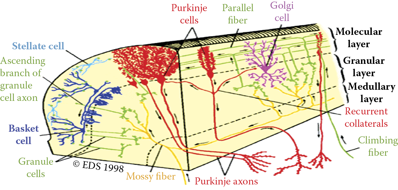
Cerebellar cortex showing that an organism’s nervous system is built of many connected neurons. The same pattern is applied in artificial neural nets.
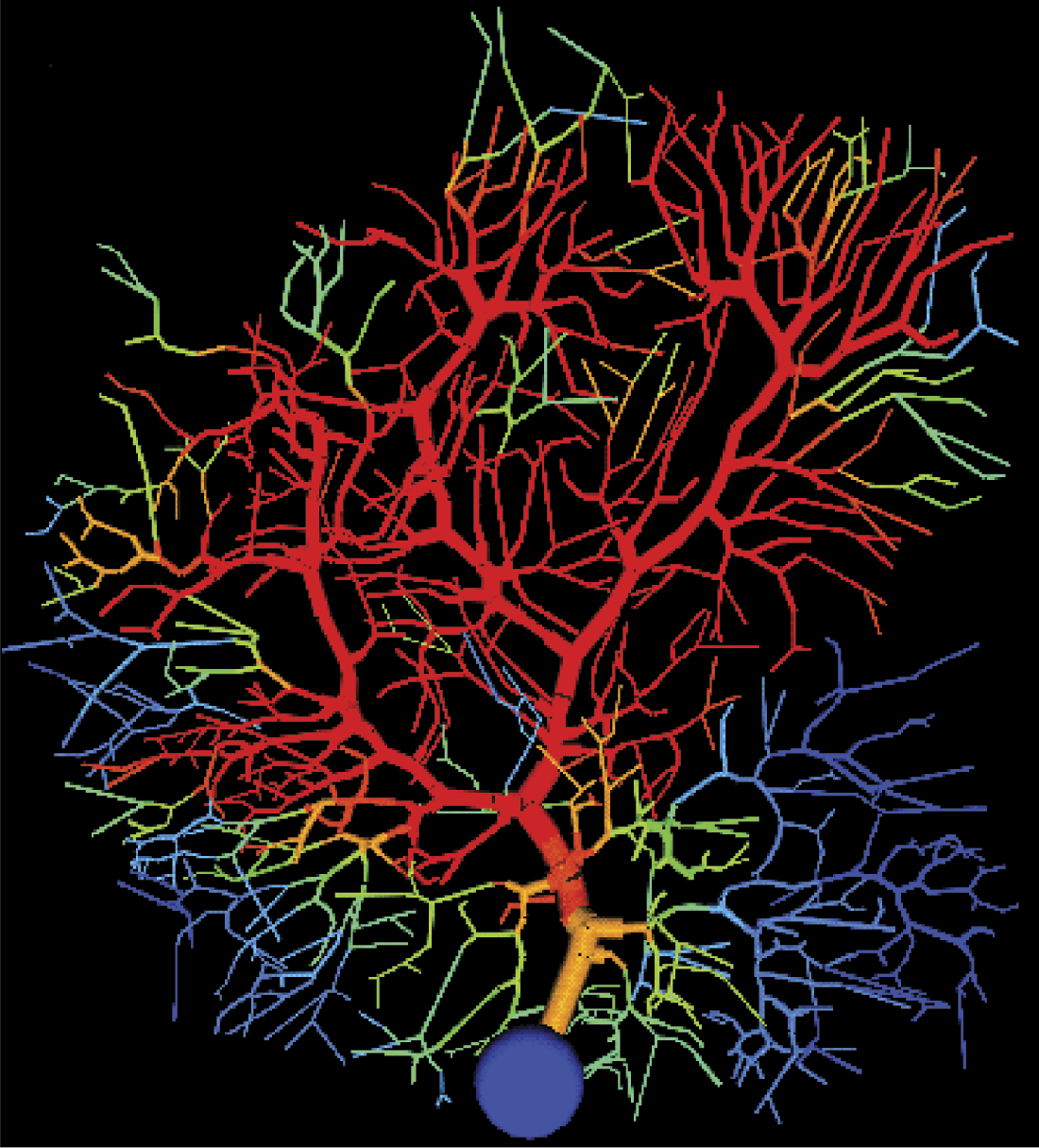
Neural networks are also built from a lot of neurons, but they are artificial—far more simple than the biological neurons and connected in a less complicated (more primitive) way. The artificial neural network model of a real nervous system structure would appear unclear and difficult to control. Figure 2.2 shows how an artificial neural net based on the identical structure scheme of a real nervous system. You can see that the structure does not appear easy to study; the structure is very complex, like a forest.
Artificial neural net with structure based on three-dimensional brain map. (Source: http://www.kurzweilai.net/images/3D-nanoelectronic-neural-tissue.jpg )
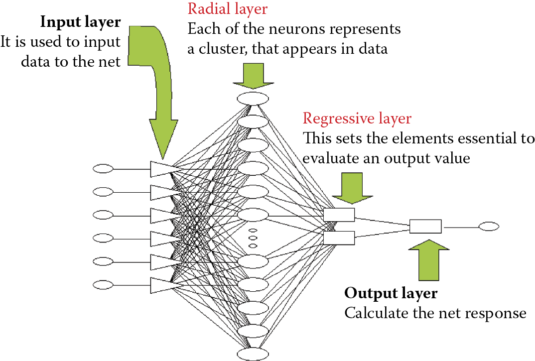
Artificial neural nets are built so that their structures may be traced easily, and production and use are economical. In general, the structures should be flat (not three-dimensional) and regular, with layers of neurons having well-defined objectives and linked according to simple (but wasteful) requirement to connect “everyone with everyone.” Figure 2.3 illustrates a common neural net [general regression neural network (GRNN) type]. Its structure is rational and simple in comparison to a biological network. We shall discuss three factors that influence neural networks properties and possibilities:
- The elements used to build a network (how artificial neurons look and work)
- How the elements are connected with each other
- Establishing the parameters of a network by its learning process
2.2 Constructing Artificial Neurons
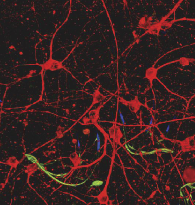
The basic building materials we use to create a neural network are artificial neurons and we must learn about them precisely. In the previous section, we illustrated biological neurons. Figure 2.4 is a simplified depiction of a neuron. To make the point that not all neurons look exactly like that, Figure 2.5 shows a biological neuron dissected from rat cerebral cortex.
Structure of a biological nerve cell (neuron). (Source: http://cdn.thetechjournal.com/wp-content/uploads/HLIC/8905aee6a649af86842510c9cb0fc5bd.jpg )
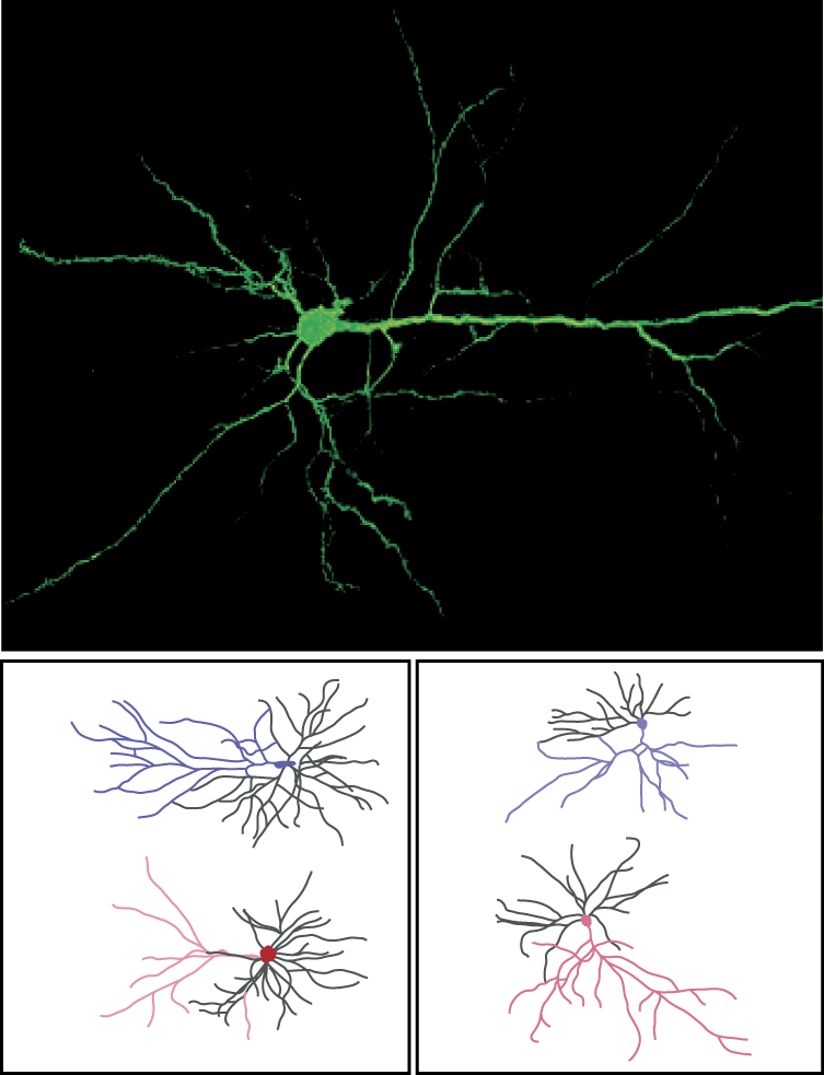
Microscopic views of real neurons. (Source: http://newswire.rockefeller.edu/wp-content/uploads/2011/12/110206mcewen.1162500780.jpg )
It is hard to distinguish between an axon that delivers signals from a specific neuron to all the others, and a dendrite that serves another purpose from the maze of fibers in the figure. Nevertheless, the figure portrays a real biological neuron that resembles the artificial neuron presented in Figure 2.6. A comparison of Figure 2.4, Figure 2.5, and Figure 2.6 will demonstrate the degree to which neural network researchers simplified biological reality.
However, despite the simplifications, artificial neurons have all the features required from the view of tasks they are supposed to carry out. Let us look at some common features of artificial neurons.
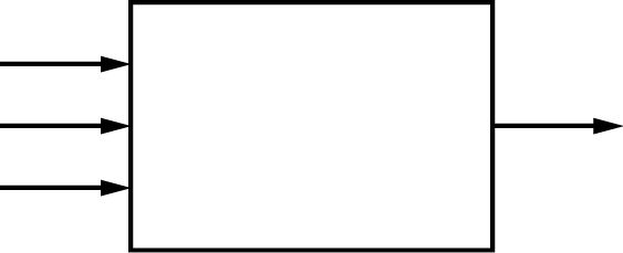
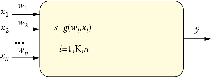
They are characterized by many inputs and a single output. The input signals xi (i = 1, 2,…,n) and the output signal y may take on only numerical values, generally ranging from 0 to 1 or from –1 to +1). The fact that the tasks to be solved contain information (e.g., the output of a decision to recognize an individual after analyzing a photo) is the result of a specific agreement. Generally each input and output is associated with a specific meaning of a signal. Additionally, signal scaling is used, so that the selected signal values within a network would not be out of an agreed range (e.g., from 0 to 1).
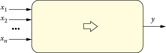
Artificial neurons perform specific activities on input signals, and consequently produce output signals (only one by a single neuron) meant for forwarding to other neurons or onto the network’s output. Network assignment, reduced to the functioning of its basic neuron element, is based on the fact that it transforms an input data xi into a result y by applying rules that are both learned and assigned at the time of network creation. Figure 2.7 illustrates these neuron properties.
Neurons have the ability to learn via coefficients called synaptic weights (Figure 2.8). As noted in Chapter 1, artificial neurons reflect the complex biochemical and bioelectric processes that take place in real biological neuron synapses. The synaptic weights that constitute the basis of teaching a network can be modified (i.e., their values can be changed). Adding adjustable weight coefficients to a neuron structure makes it a learnable unit. Artificial neurons can be treated as elementary processors with specific features described below.
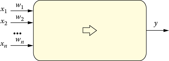
Each neuron receives many input signals xi and on the basis of the inputs, determines its answer y with a single output signal. A weight parameter called wi is connected to separate neuron inputs. It expresses a degree of significance of information arriving to a neuron using a specific input xi.
A signal arriving via a particular input is first modified with the use of the weight of the input. Most often a modification is based on the fact that a signal is simply multiplied through the weight of a given input. Consequently, in further calculations, the signal participates in a modified form. It is strengthened (if the weight exceeds 1) or restrained (if the weight value is less than 1). A signal from a particular input may occur even in the form opposite signals from the other inputs if its weight has a negative value. Inputs with negative weights are defined by neural network users as inhibitory inputs; those with positive weights are called excitatory inputs.
Input signals (modified by adequate weights) are aggregated in a neuron (see Figure 2.9). Networks utilize many methods of input signal aggregation. In general, aggregation involves simply adding the input signals to determine internal signals. This is referred as cumulative neuron stimulation or postsynaptic stimulation. This signal may be also defined as a net value.
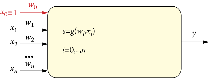
Sometimes a neuron adds an extra component independent of input signals to the created sum of signals. This is called bias and it also undergoes a learning process. Thus, a bias can be considered an extra synaptic weight associated with inputs and it is provided an internal signal of constant value equal to one. A bias helps in the formation of a neuron’s properties during the learning phase since the aggregation function characteristics need not pass through the beginning of the coordinate system. Figure 2.10 depicts a neuron with a bias.
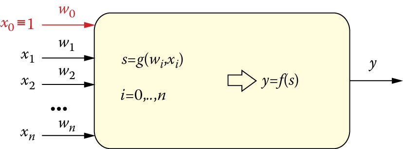
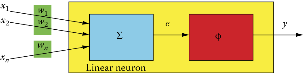
A sum of internal signals multiplied by weights plus (possibly) a bias may be sometimes sent directly to its axon and treated as a neuron’s output signal. This works well for linear systems such as adaptive linear (ADALINE) networks. However, in a network with richer abilities such as the multilayer perceptron (MLP), a neuron’s output signal is calculated by means of some nonlinear function. Throughout this book, we shall use the symbol ƒ() or φ() to represent this function. Figure 2.11 depicts a neuron including both input signal aggregation and output signal generation.
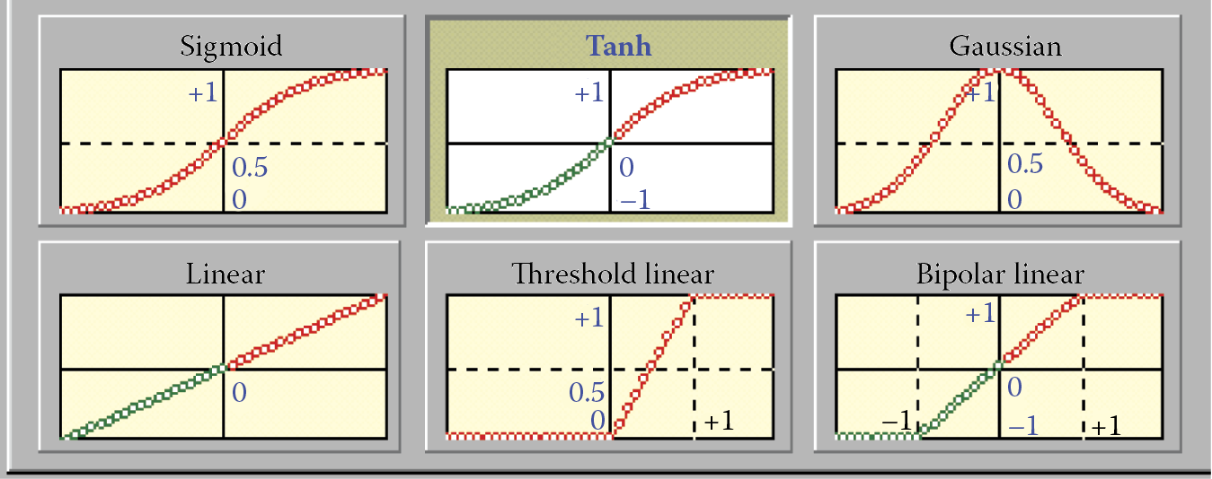
Function φ() is called a characteristic of a neuron (transfer function). Figure 2.12 illustrates various characteristics of neurons. Some of them are chosen in such a way that an artificial neuron’s behavior would be the most similar to a real biological neuron’s behavior (a sigmoid function), but characteristics also could be selected in a manner that would ensure the maximum efficiency of computations carried on by a neural network (Gauss function). In all cases, function φ() constitutes an important element between a joint stimulation of a neuron and its output signal.
A knowledge of the input signals, weight coefficients, input aggregation method, and neuron characteristics allowed to unequivocally define the output signal at any time usually assumes that the process occurs immediately, contrary to what happens in biological neurons. This helps the artificial neural networks reflect changes in input signals immediately at the output. Of course, this is a clearly theoretical assumption. After input signals change, even in electronic realizations, some time is needed to establish the correct value of an output signal by an adequate integrated circuit.
Much more time would be necessary to achieve the same effect in a simulation run because a computer imitating network activities must calculate all values of all signals on all outputs of all neurons of a network. That would require a lot of time even on a very fast computer. We will not pay attention to neuron reaction time in discussions of network functioning because the reaction time is an insignificant factor in this context. Figure 2.13 presents a complete structure of a single neuron.
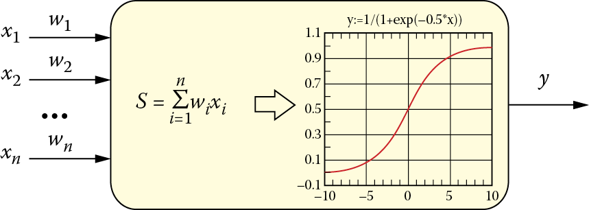
The neuron presented in this figure is the most typical “material” used to create a network. More precisely, such typical network material constitutes neurons defined as multilayer perceptrons (MLPs). The most crucial elements of the material are presented in Figure 2.14. Note that the MLP neuron is characterized by the aggregation function consisting of simple summing of input signals multiplied by weights and uses a nonlinear transfer function with a distinctive sigmoid shape.
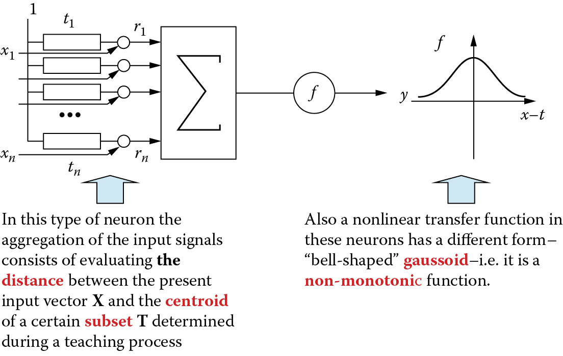
Radial neurons are sometimes used for special purposes. They involve an atypical method of input data aggregation, use a specific (Gaussian) characteristic, and are taught in an unusual manner. We will not go into elaborate details about these specific neurons that are used mainly to create special networks called radial basis functions (RBFs). Figure 2.15 shows a radial neuron to allow a comparison with the typical neuron shown in Figure 2.14.
2.3 Attempts to Model Biological Neurons
All artificial sigmoid and radial neurons described in this chapter and elsewhere in this book are simplified models of real biological neurons, as noted earlier. Now let us see the true extent of simplification of artificial neurons in reality. We shall use the example of research of Goddard et al. (2001) to illustrate this point.
For many years, de Schutter tried to model in detail the structure and working of a single neuron known as the Purkinje cell. His model utilized electric systems that, according to Hodgkin and Huxley (Nobel Prize in 1963), modeled bioelectrical activities of individual fibers (dendrites and axons) and cell membranes of neuron soma. He was successful in generating with extraordinary accuracy the shape of a real Purkinje cell after considering Neher’s and Sakamann’s research (Nobel Prize in 1991) on the functioning of so-called ion channels.
The modeled cell structure and replacement circuit used in Goddard et al. (2001) model are shown in Figure 2.16. The model turned out to be very complicated and involved costly calculations. For example, it required 1,600 so-called compartments (cell fragments treated as homogeneous parts containing specific substances in specific concentrations), 8,021 models of ion channels, 10 different complicated mathematical descriptions of ion channels dependent on voltage, 32,000 differential equations, 19,200 parameters to estimate when tuning the model, and a precise description of the cell morphology based on precise microscopic images.
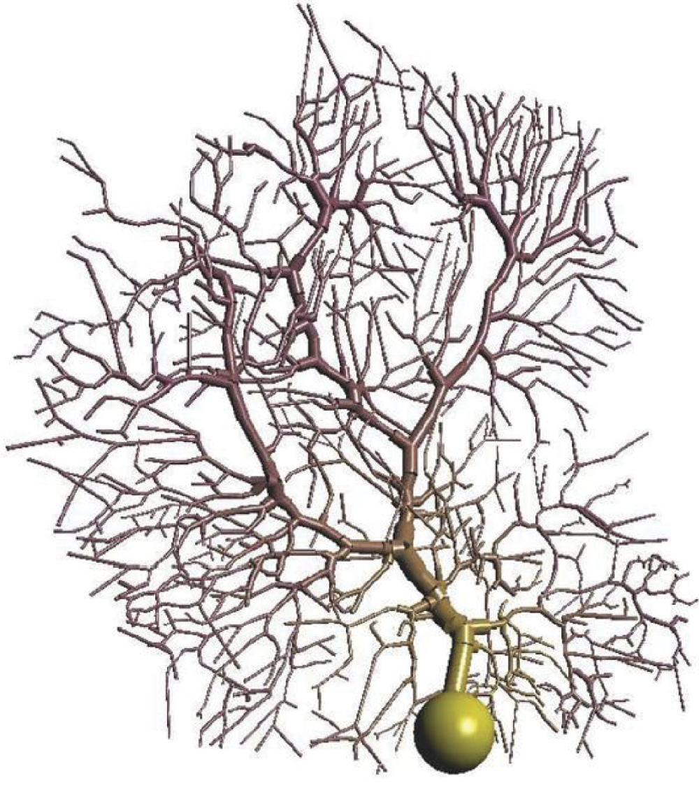
de Schutter’s model of Purkinje cell neuron that clearly resembles biological original. (Source: http://homepages.feis.herts.ac.uk/~comqvs/images/purkinje_padraig.png )
It is no surprise that many hours of continuous work on a large supercomputer were needed to simulate several seconds of “life” of such a nerve cell. Despite this issue, the results of the modeling are very impressive. One result is presented in Figure 2.17.
Example result obtained by de Schutter. (Source: http://www.tnb.ua.ac.be/models/images/purkinje.gif )
The results of these experiments are unambiguous. This attempt at faithful modeling of the structure and action of a real biological neuron was successful but simply too expensive for creating practical neural networks for widespread use.
Since then, researchers used only simplified models. Despite the extent of simplification they represent, we know that neural networks can solve certain problems effectively and even allow us to draw interesting conclusions about the behavior of human brain.
2.4 How Artificial Neural Networks Work
From the earlier description of neural networks, it follows that each neuron possesses a specific internal memory (represented by the values of current weights and bias) and certain abilities to convert input signals into output signals. Although these abilities are rather limited (a neuron is a low-cost processor within a system consisting of thousands of such elements), neural networks are valuable components of systems that perform very complex data processing tasks.
As a result of the limited amount of information gathered by a single neuron and its poor computing capabilities, a neural network usually consists of several neurons that act only as a whole. Thus, all the capabilities and properties of neural networks noted earlier result from collective performances of many connected elements that constitute the whole network. This specialty of computer science is known as massive parallel processing (MPP).
Let us now look at the operational details of a neural network. It is clear from the above discussion that the network program, the information constituting the knowledge database, the data calculated, and the calculation process are all completely distributed. It is not possible to point to an area where specific information is stored even though neural networks may function as memories, especially as so-called associative memories and have shown impressive performance. It is also impossible to relate certain areas of a network to a selected part of the algorithm used, for example, to indicate which network elements are responsible for initial processing and analysis of input data and which elements produce final network results.
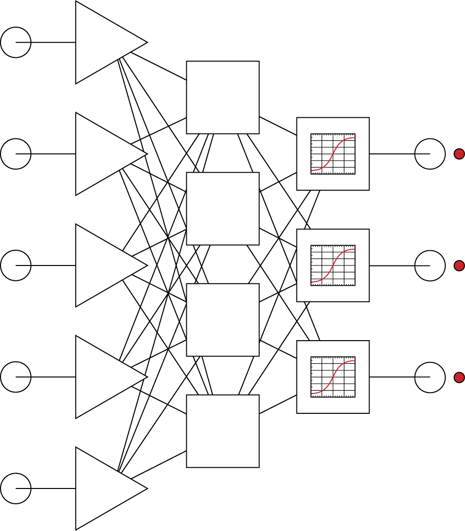
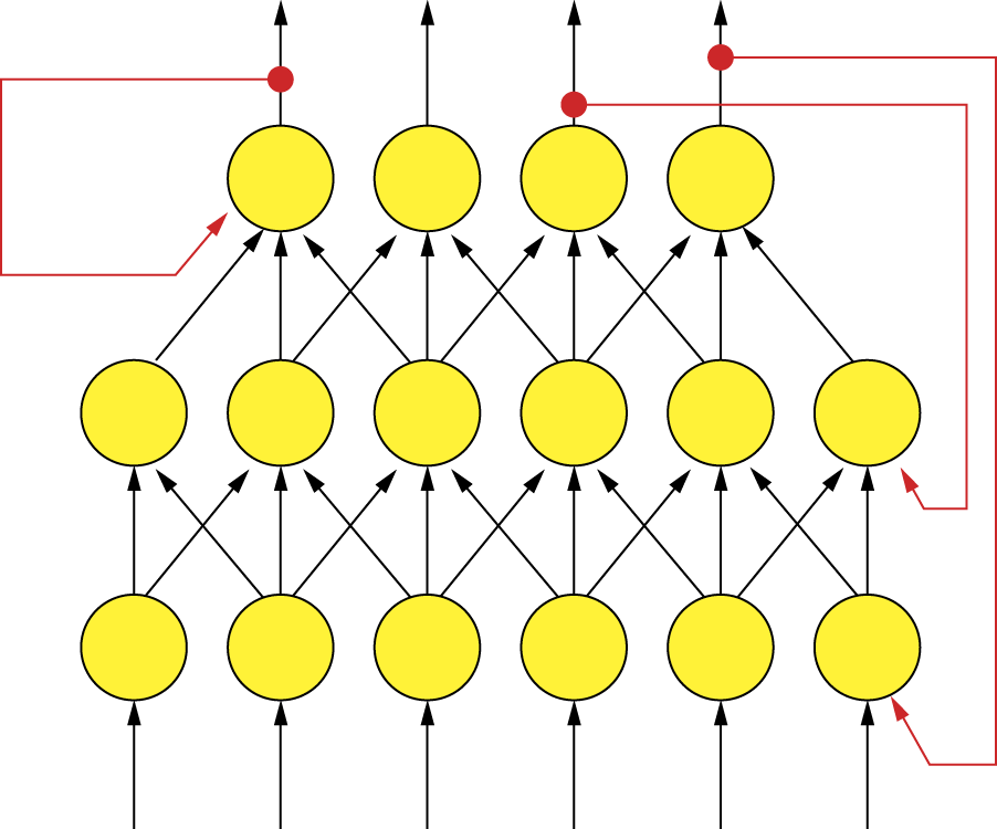
We will now analyze how a neural network works and what roles the single elements play in the whole operation. We assume that all network weights are already determined (i.e., the teaching process has been accomplished). Teaching a network is a vital and complex process that will be covered in subsequent chapters. We will start this analysis from the point where a new task is presented to a network. The task is represented by a number of input signals appearing at all input ports. In Figure 2.18, these signals are represented by red (tone) dots. The input signals reach the neurons in the input layer. These neurons usually do not process the signals; they only distribute them to the neurons in the hidden layer (Figure 2.19).
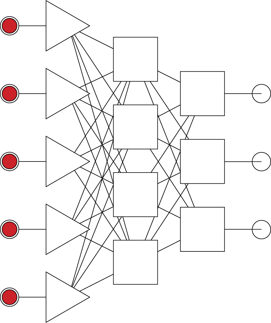
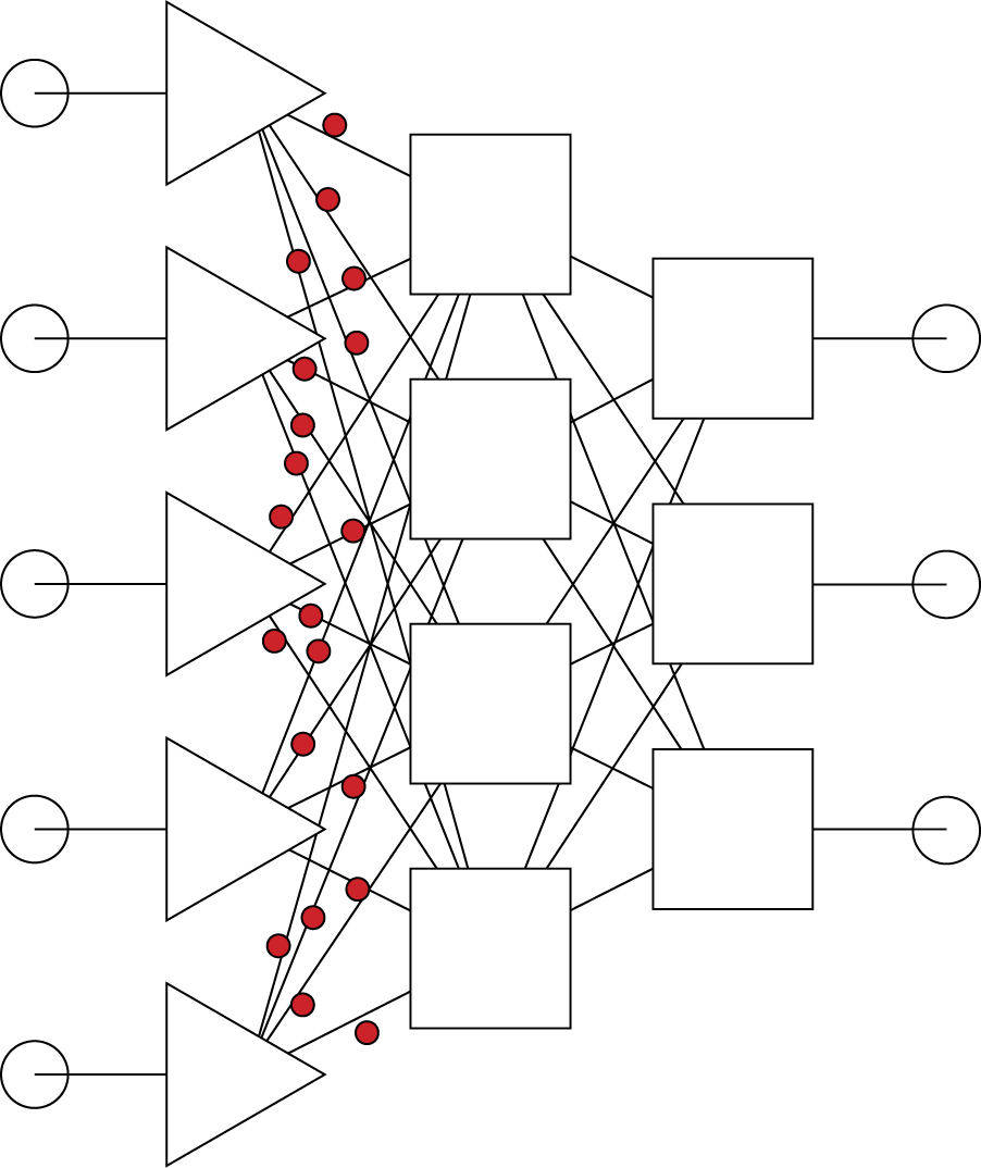
Note that the distinct nature of the input layer neurons that only distribute signals rather than process them is generally presented graphically by various types of symbols (e.g., a triangle instead of a square).
The next stage involves activation of the neurons in the hidden layer. These neurons use their weights (hence utilizing the data they contain) first to modify the input signals, aggregate them, and then, accordingly to their characteristics (shown in Figure 2.20 as sigmoid functions), calculate the output signals that are directed to the neurons in the output layer.
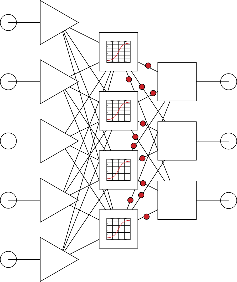
After processing signals, neurons from a hidden layer produce intermediate signals and direct them to neurons in an output layer.
This stage of data processing is crucial for neural networks. Even though the hidden layer is invisible outside the network (its signals cannot be registered at the input or output ports), this layer is where most of the task solving is performed. Most of the network connections and their weights are located between the input and the hidden layers. We can say that most of the data gathered in the teaching process is located in this layer.
The signals produced by the hidden layer neurons do not have direct interpretations, unlike input or output signals—every single signal has a meaning for the task being solved. However, using a manufacturing process analogy, the hidden layer neurons produce semiproducts, that is, signals characterizing the task in such a way that it is relatively easy to use them later to assemble the final product (the final solution determined by output layer neurons; see Figure 2.20).
Following the performance of the network at the final stage of task solving, we can see that the output layer neurons take advantage of their abilities to aggregate signals and their characteristics to build the final solution at the network output ports (Figure 2.21). In summary, a network always works as a whole and all its elements contribute to performing all the tasks of the network. The process is similar to a hologram reproduction where one can reproduce a complete picture of a photographed object from pieces of a broken photographic plate.
Neurons from an output layer use information from neurons in a hidden layer and calculate final results.
One of the advantages of network performance is its unbelievable ability to work properly even after a failure of a significant portion of its elements. Frank Rosenblatt, a neural network researcher, taught his networks certain abilities (such as letter recognition) and then tested them as he damaged more and more of their elements. The networks were special electronic circuits. Rosenblatt could damage a significant part of a network and it would continue to perform properly (Figure 2.22). Failure of a higher number of neurons and connections would deteriorate the quality of performance in that the damaged part of the network would make more mistakes (e.g., recognize O as D) but it would not fail to work.
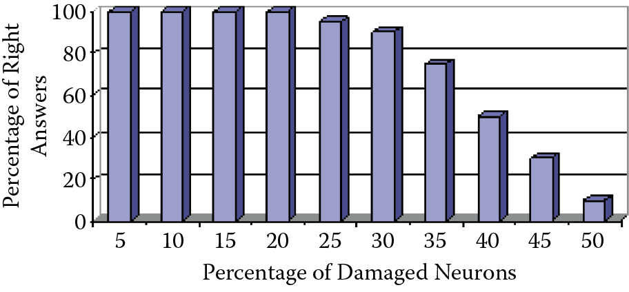
Compare this behavior to the fact that the failure of a single element of a modern electronic device such as a computer or television can cause it to stop working. Thousands of neurons within a human brain die every day for many reasons, but our brains continue to work unfailingly throughout our lives. Details of this fascinating property of the neural network are described in a paper by Tadeusiewicz et al. (2011).
2.5 Impact of Neural Network Structure on Capabilities
Let us consider now the relationship between the structure of a neural network and the tasks it can perform. We already know that the neurons described previously are used to create networks. A network structure is created by connecting outputs of neurons with inputs of other neurons based on a chosen design. The result is a system capable of parallel and fully concurrent processing of diverse information.
Considering all these factors, we usually choose layer-structured networks and connections between the layers are made on a one-to-one basis. Obviously the specific topology of a network (the numbers of neurons in layers) should be based on the types of tasks the network is to perform. In theory the rule is simple: the more complicated the task, the more neurons in a network are needed to solve it. A network with more neurons is simply more intelligent. In practice, however, this concept is not as unequivocal as it appears.
The vast literature about neural networks contains numerous works proving that the decisions related to a network’s structure affect its behavior far less than expected. This paradoxical statement derives from the fact that behavior of a network is determined fundamentally by the network teaching process and not by its structure or number of elements it contains. This means that a well-taught network that has a questionable structure can solve tasks more efficiently than a badly trained network with an optimal structure. Many experiments were performed on network structures created by randomly deciding which elements to connect in what way. Despite their casual designs, the networks were capable of solving complex tasks.
Let us take a closer look at the consequences of the statement about random design because they are interesting and important. If a randomly designed network can achieve correct results despite its structure, its teaching process allowed it to adjust its parameters to operate as required based on a chosen algorithm. This means the system will run correctly despite its fully randomized structure. These experiments were first performed in the early 1970s by Frank Rosenblatt. The researcher rolled dice or drew lots and, depending on the results, connected certain elements of a network together. The resulting structure was completely chaotic (Figure 2.23). After teaching, the network could solve tasks effectively.
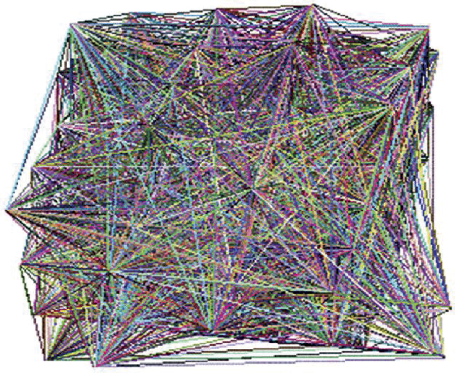
Rosenblatt’s reports of his experiments were so astonishing that scientists did not believe his results were possible until the experiments were repeated. The systems similar to the perceptron built by Rosenblatt were developed and studied around the world (Hamill et al., 1981). Such networks with random connections could always learn to solve tasks correctly; however, the teaching process for a random network is more complex and time consuming compared to teaching a network whose structure relates reasonably to the task to be solved.
It is interesting that philosophers were also interested in Rosenblatt’s results. They claimed that the results proved a theory proclaimed by Aristotle and later extended by Locke. The philosophical concept is tabula rasa. The mind is considered a blank page that is filled in by learning and life experience. Rosenblatt proved that this concept is technically possible, at least in the form of a neural network. Another issue is whether the concept works for all humans. Locke claimed that inborn abilities amounted to nothing and gained knowledge was everything.
We cannot comment on Locke’s statement but we certainly know that neural networks gain all their knowledge only by learning adjusted to the task structure. Of course, the network structure must be complex enough to allow “crystallization” of the needed connections and structures. A network that is too small will never learn anything because its “intellectual potential” would be inadequate.
The important issue is the number of elements, not the structure design. For example, no one teaches relativity theory to a rat although a rat may be trained to find its way through complicated labyrinths. Similarly, no human is programmed at birth to be a surgeon, an architect, or a laborer. Careers and jobs are choices. No statements about equality will change the fact that some individuals have remarkable intellectual resources and some do not.
We can apply this idea to network design. We cannot construct a network with inborn abilities although it is easy to create a cybernetic moron that has too few neurons to learn. A network can perform widely diverse and complex tasks if it is big enough. Although it seems that a network cannot be too large, size can create complications as we will see in Section 2.13.
2.6 Choosing Neural Network Structures Wisely
Despite studies indicating that a randomly constructed network can solve a problem, a formalized neural structure is obviously more desirable. A reasonably designed structure that fits the problem requirements at the beginning can significantly shorten learning time and improve results. That is why we want to present some information about construction of neural networks even though it may not provide solutions for all kinds of construction problems.
Choosing a solution to a construction problem without sufficient information is very difficult if not impossible. Placing a neural network constructor in a situation that allows it to adopt any structure freely is similar to the problem of the abecedarian computer engineer who is confused by the “press any key” system message. Which key? You may laugh about that but we hear a similar question from our graduate students: what is “any structure” of a neural network?
We must note a few facts about common neural network structures. Not all aspects of all structures are completely understood. Designing a neural network requires both cerebral hemispheres to deal with the logical and creative issues. We start by classifying commonly used neural network structures into two major classes: neural networks with and without feedback. Neural networks without feedback are often called feed-forward types. Networks in which signals can circuit for unlimited time are called recurrent.
The feed-forward networks follow a strictly determined direction of signal propagation. Signals go from defined input, where data relevant to the problem arrives in the neural network, to output where the network produces a result (Figure 2.24). These types of networks are the most common and useful. We will talk about them later in this chapter and elsewhere in this book.
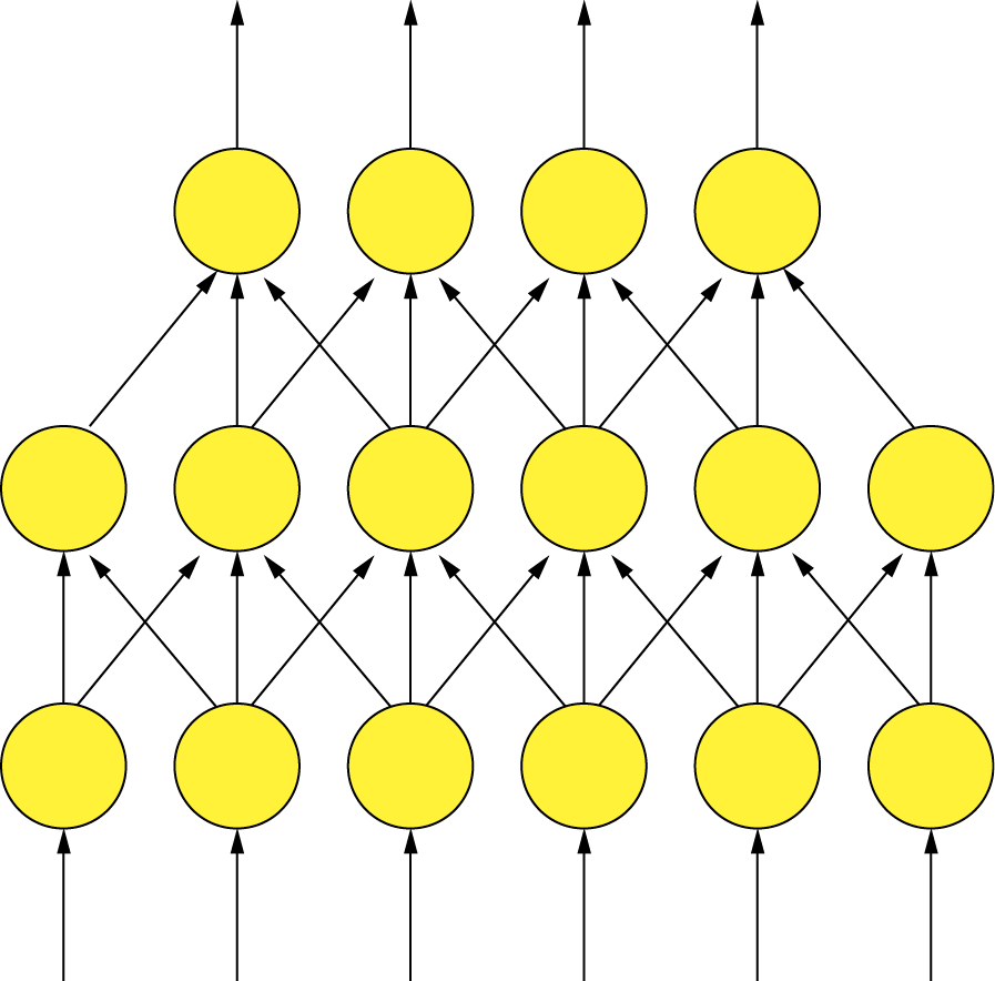
Example structure of a feed-forward neural network. Neurons represented by circles are connected to allow transmission signals only from input to output.
The recurrent networks are characterized by feedback (Figure 2.25). Signals can circuit between neurons for a very long time before they reach a fixed state. In some cases, these networks do not produce fixed states. In Figure 2.25, the connections presented as red (outer) arrows are feedbacks so the network depicted is recurrent.
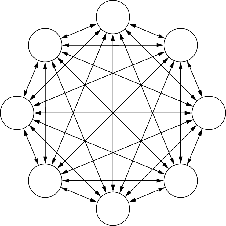
Recurrent network properties and abilities are more complex than feed-forward networks. Furthermore, their computational potentials are astonishingly different from those of other types of neural networks. For instance, they can solve optimization problems. They can search for best possible solutions—a task that is almost impossible for feed-forward networks. Among all recurrent networks, a special place belongs to those named after John Hopfield. In Hopfield networks, the one and only type of connection between neurons is feedback (Figure 2.26).
Some time ago, the solution of the famous traveling salesman problem by a Hopfield network was a global sensation. Given a set of cities and the distance between each possible pair, the traveling salesman problem is to find the best possible way of visiting all the cities exactly once and returning to the starting point. A solution of this problem using neural networks was presented for the first time in a paper by Hopfield and Tank (1985). Afterward, the problem has been discussed many times in numerous papers (e.g., Gee and Prager, 1995). One recently published paper about using neural networks for solving the traveling salesman problem was authored by Wang, Zhang, and Creput (2013). The event opened a path for Hopfield networks to manage the important NP-complete (nondeterministic polynomial time) class of computational problems, but this is something we will discuss later. Despite this sensational breakthrough, Hopfield networks did not become as popular as other types of neural networks, so we will cover them in Chapter 11.
Building a neural network with feedbacks is far more difficult than constructing a feed-forward net. Controlling a network involving multiple simultaneous dynamic processes is also much more difficult than controlling a network where signals uniformly go from input to output. For this reason, we will start with one-directional signal flow networks and then progress to recurrent nets.
If we focus on feed-forward networks, the best and most common way to characterize their structure is a layer model in which we assume that neurons are clustered in sets called layers. Major interlinks exist between neurons in adjacent layers. This kind of structure is mentioned early in the chapter, but is worth another look (Figure 2.27).
As noted earlier, links between neurons from adjacent layers may be constructed in many different ways but the most common configuration is all-to-all linkage. The learning process will cut off unneeded connections automatically by setting their coefficients (weights) to zero.
2.7 “Feeding” Neural Networks: Input Layers
Among all layers that constitute a neural net, we begin with the input layer whose purpose is to collect and convert data outside the network (tasks to be completed, problems to be solved) to inputs. The input layer decision is fairly easy. The number of elements in the layer is determined strictly by the amount of incoming data to be analyzed for a specific task or problem. However, sometimes decisions about which and how many data should be fed to a neural net become quite complex.
Assume, for example, that we want to predict how stock indices will behave. It is well known that some researchers achieve encouraging results that surely produce increased income for those willing to take risks by selling or buying stocks based on outputs produced by neural nets. However, publications revealing data used as inputs are harder to find. Neural nets are applied after they master learning routines.
Users receive outputs in the forms of colorful graphs showing how well the stocks performed. Inputs are described vaguely, for example, “The network utilized information about earlier stock returns and financial analysis documentation.” Obviously, preparation and results are explained, but the actual operation of such networks remains an interesting secret.
Another important yet subtle issue is that numeric inputs and outputs are usually limited. Most implementations assume all neuron inputs to be digits from 0 to 1 (or better, from –1 to +1). If we require results outside that range, we need scaling (Figure 2.28).
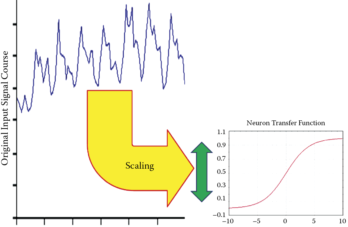
The problem with scaling inputs is actually less important than dealing with results as shown in the next section. Inputs may be assigned any signal with any value. However, outputs are defined by neuron characteristics. Neurons can produce only signals for which they are programmed. To preserve unitary interpretation of all signals in a neural network and assign importance weights, we usually scale output data. Scaling also aids normalization of input variables.
It is difficult to guarantee network equivalency of input signals. The main problem is that the values of some important variables are naturally very small, whereas other less important variables produce high values. Inputs of a neural net used by a doctor to help diagnose patients could be levels of erythrocytes (red blood cells) and body temperature. Both variables are equally important to the network although the doctor may be influenced by one value or the other. However, human body temperature is generally a low number (36.6 degrees Celsius for a healthy man) and even its slight changes up or down may indicate serious health issues.
The number of red blood cells is normally about 5 million. A difference of a million cells is not a cause for alarm. Remember scaling? A neuron seeing two inputs at different levels would ignore the difference. Normalization or scaling allows us to treat every input according to its importance defined by the neural net creator rather than its numerical value.
2.8 Nature of Data: The Home of the Cow
The next problem is more difficult. Data provided to a neural network or generated by it as a result of solving a problem may not always be numerical nature. Not everything in our world can be measured and described numerically. Many data to be used as inputs into or outputs from a neural network have a qualitative, descriptive, or nominal nature. This means that their values are represented by names instead of numbers. As an example, assume your task is to design a neural network to distinguish whether certain animals may or may not be dangerous to humans. (We have published similar problems on the Internet.)
The task needs inputs, for example, the part of the world where the animal lives. If an animal is big, has horns, and gives milk, it is probably a cow. What determines whether it is dangerous is the continent where it lives. European and Asian cows are calm and mellow as a rule. Some American cows reared on open pastures are dangerous. Therefore, to decide whether an animal is or is not dangerous, the task involves a variable that indicates an animal’s origin. However, how do we distinguish Asia from America as inputs of a neural network?
A solution for the input problem is use of a representation called one of N where N denotes the number of different possible values (names) that the nominal variable may adopt. Figure 2.29 shows a coding system for the one of N method in which N = 3. The principle is simple and involves using for every nominal variable as many neurons in an input layer as different values of a specific variable may adopt (which is simply N). If, for example, we assume that an animal may come only from Asia, America, or Europe, we must designate a set of three neurons to represent the origin variable. We then we want to inform a network that in this case one origin variable is the America name. We assign a signal of value 0 to the first input, 1 to the second input, and 0 again to the third input.
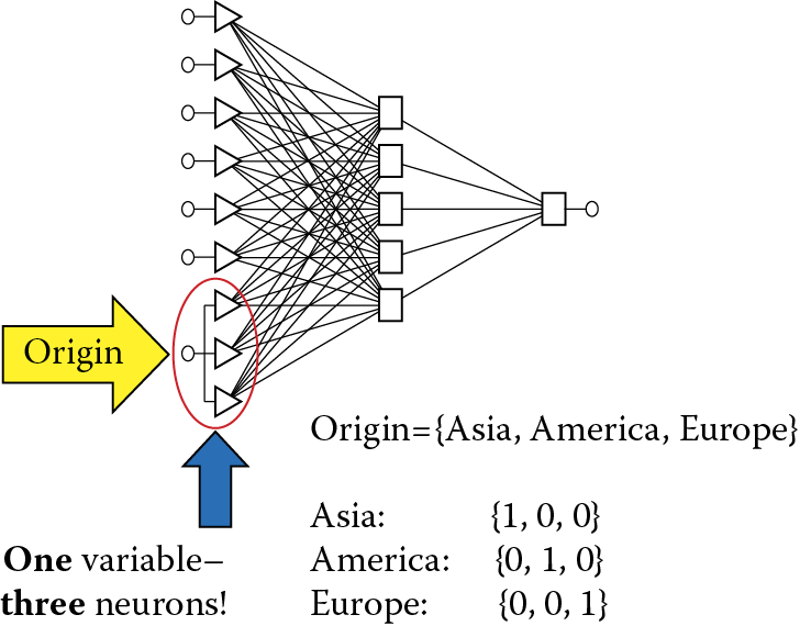
You may ask: why complicate things? Perhaps a better idea is to code Asia as 1, America as 2, and Europe as 3, then assign the values to one input of the network. If the signal on the input assumes values ranging from 0 to 1, let Asia be 0, America be 0.5, and Europe be 1. Why has no one thought of this earlier?
The hypothetical solution proposed above is unsatisfactory. Neural networks are very weak in the area of analyzing values shown to them. If you adopt the 1, 2, 3 coding system, a neural network in the learning phase will assume Europe is three times more valuable or larger than Asia and that is nonsensical. Even worse will be the application of scaling to the problem. That will indicate that America can be converted to Europe (by multiplying by 2) and Asia cannot be converted because 0 multiplied by any number always totals 0.
In brief, all nominal values have to be represented with the one of N technique even though this will increase the number of inputs, connections, and layers of a network. Of course this is inconvenient, because every connection in a network is related to a weight coefficient whose value must be determined in the course of teaching. Additional inputs and connections require more teaching. In spite of this inconvenience, no better solution exists at present. A designer must multiply inputs related to every nominal variable by using the one of N schema until a better method is devised.
One more point must be considered: an exception to the one of N rule that arises when N = 2. One binary nominal variable may be gender for which we can code male = 0, female = 1 or vice versa, and a network will cope with it. However, this kind of binary data is the exception that proves the rule that nominal data should be coded by the one of N method.
2.9 Interpreting Answers Generated by Networks: Output Layers
The second component we will discuss in this chapter is the output layer that generates the solutions to the problem considered. The solutions take the form of output signals from the network. Thus, their interpretation is vital because we must understand what the network wants to tell us.
Determining the number of exit neurons is simpler than deciding the number of entrance signals because we usually know how many and what kinds of solutions we need. Thus we have no need to deal with the steps of adding or dropping signals required for designing input layers. Coding procedures are similar for both the input and output layers. The numerical variables should be scaled to allow the neurons at the output layer to produce a number that represents the correct solution to a problem. The nominal values to be presented as outputs should follow the one from N method. However, a few typical problems arise in the output layer, as discussed below.
The first problem arises directly from use of the one from N method. Recall that the signal with maximum value (usually 1) in this method can have only one neuron on exit—a name represented as a value of a nominal variable. All remaining neurons representing one variable group should have values equal to zero. This ideal situation in which the nominal variable at the output layer is correctly indicated is shown in Figure 2.30. The convention used is that the network is (in some sense) a reversal of the task in Figure 2.29. In that case, the input requirement was the name of the continent where the classified animal lives as the first step in determining whether the animal is dangerous. An animal entry must indicate the continent where it lives.

The situation shown in Figure 2.30 is theoretical; it could happen in practice only as a result of a favorable coincidence. In practice, considering the limited precision of computations performed by networks (discussed below), neuron outputs often include a nominal variables with non-zero signals as shown Figure 2.31. What should we do about this?

To obtain clear and unequivocal answers in such situations, some additional criteria may be useful in working with network outputs. These additional criteria for post-processing of results are known as the threshold of acceptance and threshold of rejection. The exit signals computed by the neurons belonging to output layer of the network are, according to this concept, quantified by comparison of their current values with thresholds as shown in Figure 2.32.
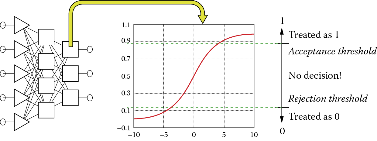
Result of output signal post-processing showing unambiguous result values despite inaccurate neuron output values.
The values of the threshold of acceptance and threshold of rejection parameters can be chosen to meet user needs. Experience shows that it is better to set high requirements for a network without trying by force to determine unequivocal values of exit variable nominals, for example, in situations of low clarity as in Figure 2.33. It is also wise to admit that a network is not able to achieve an unequivocal classification of the input signal than to accept a network decision that is probably false.
2.10 Preferred Result: Number or Decision?
While using a neural network, we must remember that results returned by the network even if they are numeric values (that may be subject to appropriate scaling) are always approximate. The quality of the approximation can vary, but significant figures should be accurate.
Accuracy is good if a product returned by a neuron has accuracy higher than two significant figures, which also means that the fault can reach several percent. That is the nature of the tool. Awareness of such limitations dictates an appropriate interpretation of the output signals so that they can be useful and also induces thinking about which neural calculations model should be used. Generally, neural networks can form regressive and classification models. In a regressive model, the output of the network must generate a specific numeric value that represents a solution of the problem. Figure 2.34 presents an interpretation of such a model.
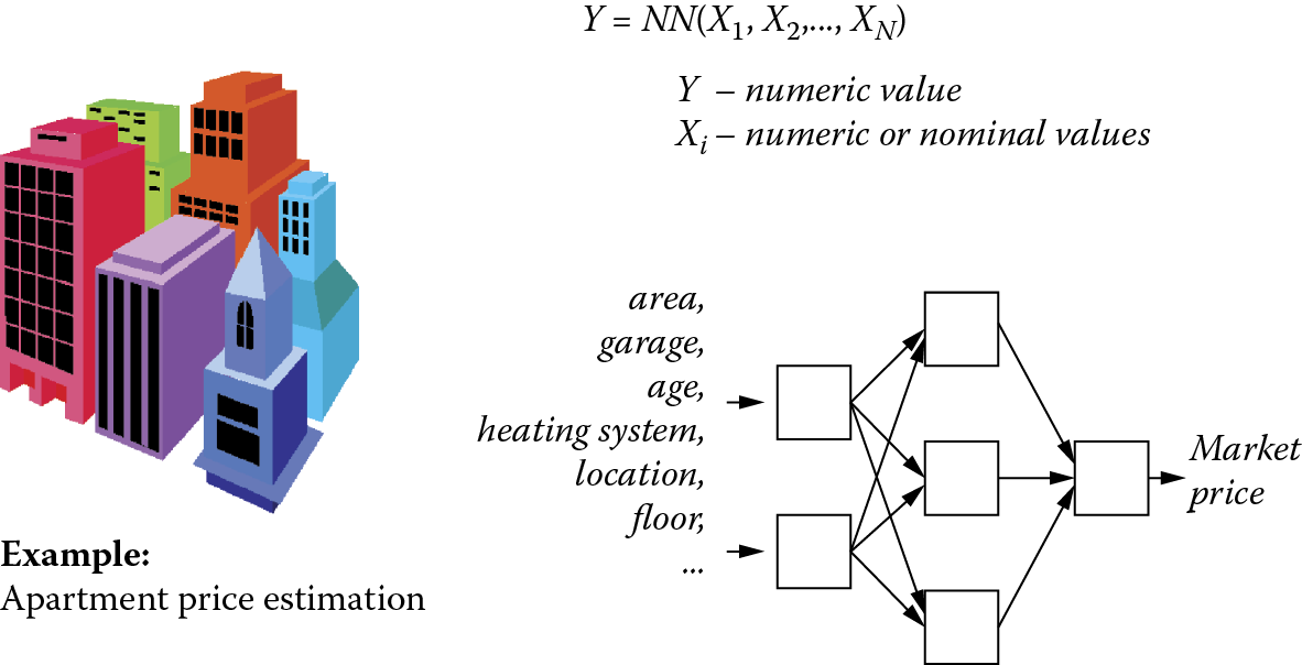
In Figure 2.34, the task of the neural network is to estimate the price of an apartment. At the input, we load data that can be numeric values (e.g., area in square meters) and data that are nominal (e.g., whether an apartment has an assigned garage). Conversely, we expect the output to be a numeric value indicating the amount that may be gained from a sale. As all apartment buyers and sellers know, a market price depends on many factors. No one can present strict economic rules for predicting absolutely accurate apartment prices. Accurate prediction is seemingly impossible because price is determined by a combination of market factors, decisions made by buyers and sellers, and timing. Still it appears that a neural network after long training (based on historical buy and sell transaction data) can form a regressive model of the problem so efficient that real prices for successive transactions may differ from predicted prices by only a few percentage points.
The alternative classification model requires information for classifying an object described by input data to one of the predefined classes. Of course, in this type of problem, a nominal output variable will be assigned (Figure 2.35). The example in the figure concerns the classification of individuals of companies seeking bank loans. Potential borrowers must be classified by a bank worker in one of two categories:
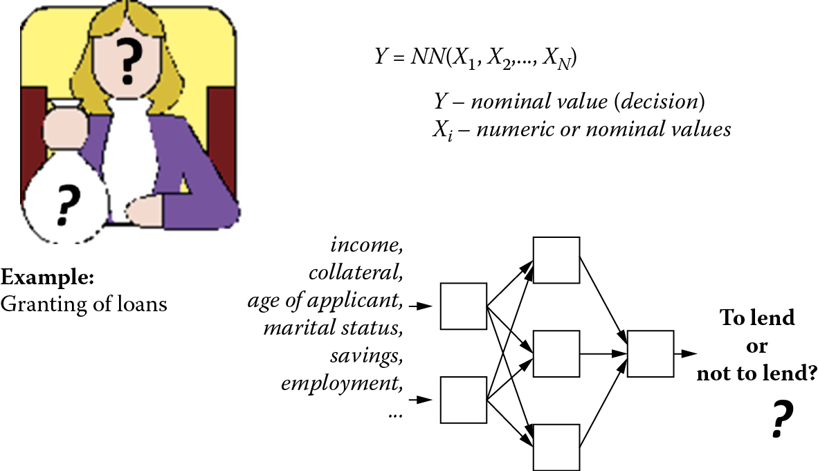
- Clients who are trustworthy and reliable, who will repay loans with interest and thus generate bank profits.
- Fraudulent applicants and potential bankrupts who will not repay their loans, thus exposing the bank to losses.
How can one distinguish one category from the other? While no strict rules or algorithms exist for this question, a correct answer can be provided by a neural network taught with historical data. Banks grant many loans and compile complete data on clients who have and have not repaid their loans and thus have a lot of relevant history information.
Years of experiences in neural network exploitations proved that it is most convenient to interpret the tasks given to a neuron network computer in a way that would allow answers utilizing the classification model. For example, we can specify that a network will state the profitability of an investment as low, average, or high or classify as borrower as reliable, risky, or totally unreliable. However, demanding that a network estimate the amount of profit, determine a risk level, or limit the amount loaned to a customer will inevitably lead to frustration because in general a neural network cannot perform these tasks. That is why the number of the outputs of a network usually exceeds the number of questions posed. This happens because we must add a few artificial neurons to service all output signals to allow the predicted range of output signal values to be divided into certain distinct subranges essential for the user. We should not force a network to return a specific “guessed” value as an output. Instead, each output neuron is responsible for signalizing a certain answer within a specific range and usually that is all we need.
Such classification networks are easy to build and teach. Constructing a neural network intended to “squeeze out” specific answers to mathematical problems is time consuming and yields minimal practical application. These issues are illustrated by Figure 2.36, which presents a “classic” neural network problem: prediction of currency rates.
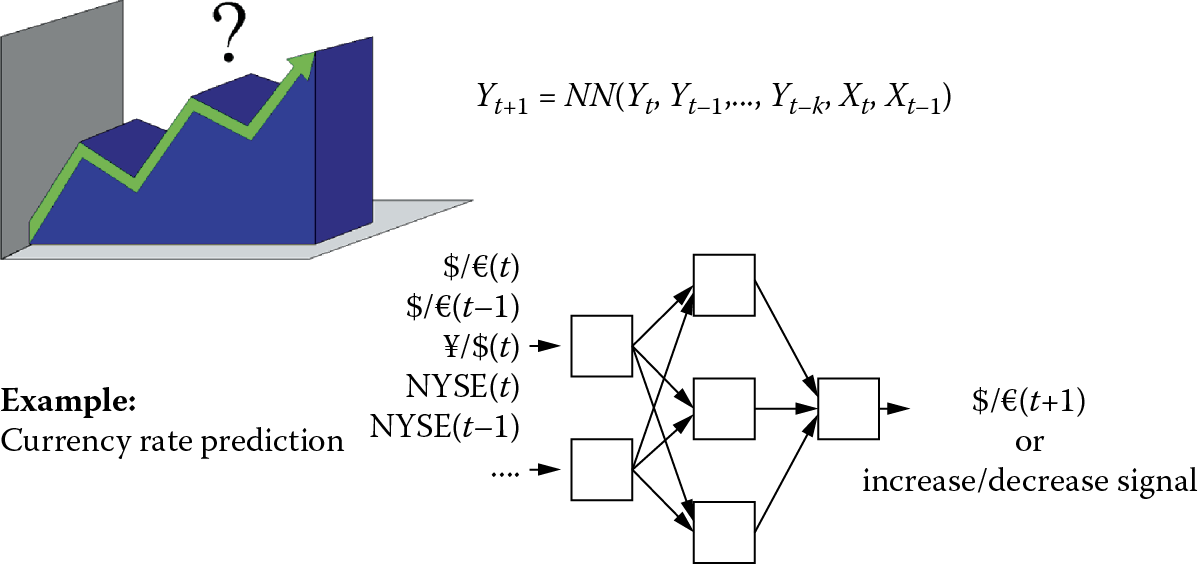
Currency rate estimation is one of many problems that require the creator of a neural network to choose between regressive and classification models. As shown in Figure 2.36, the problem can be solved in two ways: A designer can build a prognostic model that attempts to determine how many euros a dollar will be worth tomorrow or he or she can be satisfied with a model that will only indicate whether the exchange rate will rise or fall tomorrow. The second task is far easier for a network to solve and the prediction of exchange rate rise or fall can be useful for an individual who wants to exchange currency before traveling abroad.
2.11 Network Choices: One Network with Multiple Outputs versus Multiple Networks with Single Outputs
Another issue related to the design of output layers of neural networks can be solved in two different ways. It is possible to create a network producing any number of outputs to generate sufficient data to solve a problem. Increasing outputs is not always an optimal solution because the teaching of a multiple-output network, while estimating weight values, requires specific compromises that always have negative effects on results.
One example of such a compromise is deciding the role of a neuron in the calculation of the values of several output neurons that receive output signals from neurons while setting a problem for a specific neuron of the hidden layer. It is possible that the role of a given hidden neuron, optimal from the view of generating one output signal from an entire network, will be significantly different from its optimal role for another output.
In such cases, the teaching process will change the weight values in this hidden neuron by adapting it each time to a different role. This will necessitate more teaching that may not be completely successful. That is why it is better to divide a complex problem into smaller subproblems. Instead of designing one network to generate multiple outputs, it is more useful to build several networks that will use the same set of input data but contain separate hidden layers and produce single outputs.
The rule suggested in Figure 2.37 cannot be treated as dogma because some multiple-output networks learn better than those with single outputs. This paradox may not have to be solved. The potential “conflict” (described above) connected to functioning of the hidden neurons and assignment of their roles for calculating several different output values may never occur.
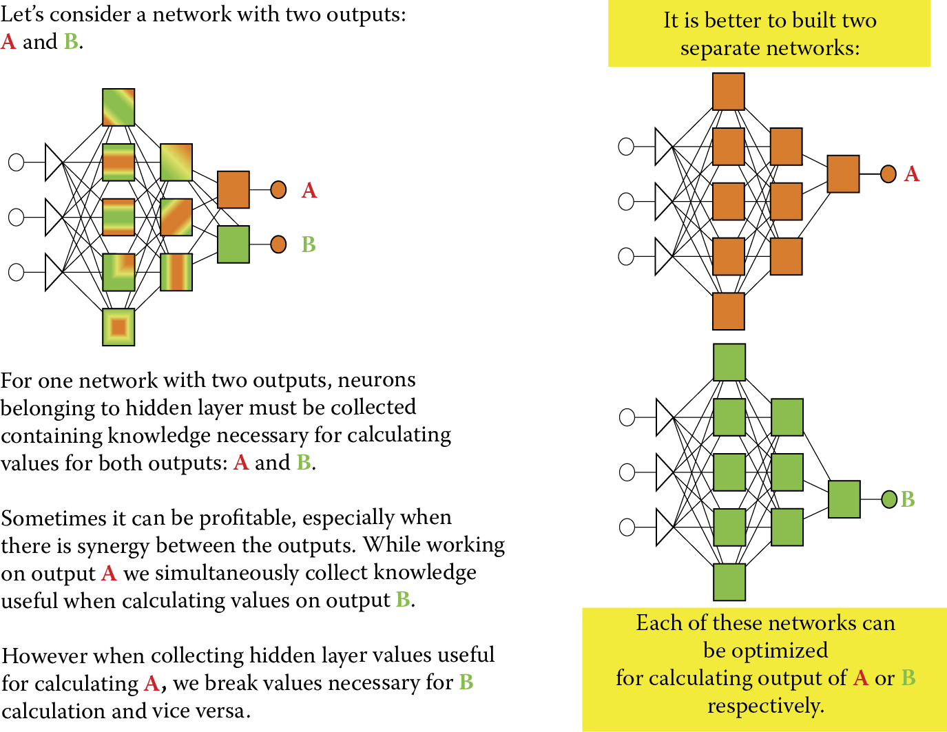
On the contrary, during the teaching process a designer can sometimes observe a specific synergy in setting the parameters of a hidden neuron that are optimal from the view of the “interests” of several output layer neurons. One can achieve success faster and more efficiently with multiple-output networks than with individual networks tuned for each separate output signal.
To decide which solution works best, we recommend testing them both, then making a choice. Our observations, based on experience in building hundreds of networks for various uses and years of examining works by our students, shows that significantly more often a collection of single-output networks is an optimal solution although biological neural networks are more often organized as multi-output aggregates.
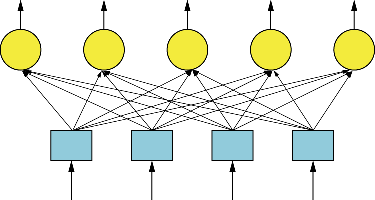
You already know that every feed-forward network requires at least one input layer and one output layer. However, single-layered networks (see Figure 2.38) utilize only one learning layer. It is, of course, an output layer because input layers of networks do not learn. Many networks, especially those solving more complex problems, must contain additional layers connecting inputs and outputs. They are installed between input and output layers and designated hidden layers. The name sounds mysterious. For that reason we will explain in what sense these layers are hidden
2.12 Hidden Layers
Hidden layers are the tools used to process input signals (received by the input layer) to the output layer in such a way to allow the required response (problem to be solved) to be found easily. Hidden layers are not utilized in every network. If they are present, they cannot be observed by users who assign tasks to a network and then make sure the network performs them correctly.
The user has no access to enter the neurons of hidden layers. He or she must use the input layer neurons to transmit signals to hidden layers. Furthermore, the user cannot access outputs. The effects of hidden layer neurons are revealed only indirectly, via the responses they produce and transmit to the output layer neurons. These layers are “hidden” in the sense that their activities are not directly visible to network users.
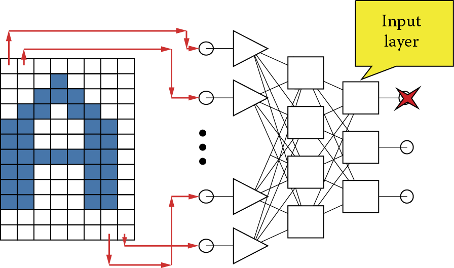
Although they are not accessible, these additional layers in neural networks handle a very important function. They create an additional structure that processes information. The simplest way to explain their role is to use the example of network implementation frequently used for pattern recognition tasks. A digital image is produced at the input (first) layer of the network.
The image cannot be a typical camera photo or traditional image loaded into a scanner or frame grabber. The reason is very simple. In a system fed by a simple image at the input (see Figure 2.30), the input layer neurons corresponds to the size and organization (grouping of neurons in corresponding rows and columns) of the image.
Briefly, each point of the image is assigned to the input of a neuron network that analyzes and reports its status. An image from a digital camera or scanner is a set of millions of pixels. It is impossible to build a network with millions of input neurons because it would require billions of connections (!) that would need set weight values. Such a structure is impossible. However, you can imagine a system that processes simplistic digital images consisting of small numbers of pixels arranged in the form of simple characters such as letters as inputs (Figure 2.39).
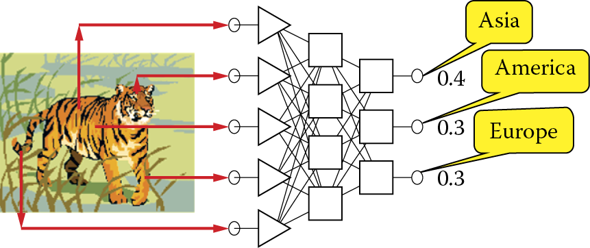
The output of the network that is expected to provide certain decisions may be organized so that the outputs of individual neurons assign certain decisions, for example, “A was diagnosed” or “B was diagnosed.” The sizes of the signals at these outputs will be interpreted in terms of the degree of certainty of the decision. Note that it is therefore possible for a network to generate ambiguous responses (“x is related to A to the extent of 0.7 and to B to the extent of 0.4 points”). It is one of the interesting and useful features of neural networks that they can be associated with fuzzy logic systems. More comprehensive discussion of this topic goes beyond the scope of this book.
Hidden layer neurons act as intermediaries. They have direct access to the input data and can see the image presented at input. Based on their outputs, additional layers make certain decisions based on certain images. It appears that the role of the hidden layer neurons is to devise pre-processed sets of input data for use by the output layer neurons in determining the final result.
The utility of the intermediate layers arises because certain input transformations make the solution of a network task much easier to achieve than attempts to solve the same task in a direct way. Using a pattern recognition task as an example, it is difficult to find a rule that allows identification of an object when only bright and dark pixels appear in an image. Finding the correct recognition rule that functions at that low level is difficult because the subjects may vary widely in shape but convey the same meaning.
A single object (e.g., the letter A) can look different when scanned from a manuscript, printed on a page, and photographed on a fluttering banner. A printed document containing exactly the same characters can be represented as two completely different pixel images due to pixel values at selected points. A slight movement can change a digital picture in a dramatic way if specific pixels are only white or black. Another difficulty with digital images of low resolution arises when completely different objects display very large sets of identical pixels on digital images.
The expectation that a “one-jump” neural network will overcome these discrepancies between the raw image and the final recognition decision may be unrealistic in some situations. The reasoning is correct because experience confirms that no learning process can ensure that a simple network with no hidden layer will be able to solve every task. Such a network without hidden layers would produce a mechanism by which some selected and established sets of pixels would be treated as belonging to different objects and at other times would link different sets pixels to the same object. This simply cannot be done.
What is not possible for a network with few layers can generally be achieved by a network containing a hidden layer. For complex tasks, neurons in the hidden layer would find certain auxiliary values that significantly facilitate solution of a task. In a pattern recognition task, hidden layer neurons can detect and encode a structure describing the general characteristics of the image and objects within the image. These characteristics should be more responsive to the demands of the final image recognition than the original image. For example, they can be to an extent independent of the position and scale of recognized objects. Examples of features that describe the objects in images of letters (to facilitate their recognition) may be:
- The presence or absence of closed contour drawing letters (letters O, D, A, and a few others; letters such as I, T, S, N, and others do not have these characteristics)
- Whether the character has a notch at the bottom (A, X, K), at the top (U, Y, V, K), or at the side (E, F)
- Rounded (O, S, C) or severe (E, W, T, A) shape
Obviously you can find many more differentiating features of letters that may or may not be insensitive to common factors affecting their recognition (font changes, handwriting, letter size changes, tilting, and panning). However, it should be emphasized that the creator of a neural network does not have to explicitly ask what characteristics of a picture may be found because the network can acquire relevant identification skills during the learning process.
Of course, we have no guarantee that a neural network designed to recognize letters taught its hidden layers to detect and signal precisely the characteristics cited above. A neural network would not detect the characteristics for differentiating letters mentioned above without sufficient training. The experiences of many researchers confirm that neural networks can recognize characteristics that effectively facilitate recognition when performing recognition tasks, although the user of a network cannot understand the relevance of characteristics encoded in hidden layers.
Hidden layers allow a neural network to perform more intelligently by utilizing elements that can extract descriptive image features precisely. Note that the nature of the extracted features is determined by the structure of the network only through the process of learning. In a network designed to recognize images, all features that will be extracted by hidden layer neurons may adapt automatically to the types of recognizable images. If we ask the network to detect masked rocket launchers in aerial photographs, it becomes clear that the main task of the hidden layer will become independent of the position of the object because the shape of the suspect can occur in any area of the image and should always be recognized in the same way.
If a network has to recognize letters, it should not lose information about their positions. A network that will detect an A somewhere on a page is not very useful because the user wants to know where the A is and in what context. In this case, the objective of the hidden layer is to extract features that may allow reliable identification of letters regardless of their size or typeface (font). Interestingly, both these tasks can be achieved after appropriate training by the same network. Of course, a network taught to recognize tanks cannot read printed material and a network trained to identify fingerprints cannot handle face recognition.
2.13 Determining Numbers of Neurons
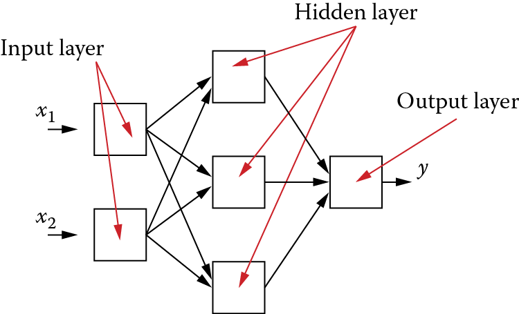
It follows from the above that the broadest possibilities for future use involve networks structured with at least three layers: (1) an input layer that receives signals, (2) a hidden layer that elicits the relevant characteristics of input signals, and (3) an output layer that makes decisions and provides a solution. Within this structure, certain elements must be determined: the numbers of input and output elements and the methods of connecting successive layers. However, certain variable elements may need to be considered: (1) the number of hidden layers and (2) the number of elements within the hidden layer or layers (Figure 2.40).
The most important problem for neural network design concerns the number of hidden neurons.
Despite many years of development of this technology, no precise theory of neural networks has yet been formulated. Network elements are usually chosen arbitrarily or by trial and error. It is possible that a designer’s concept of how many hidden neurons to use or how they should be organized (as one hidden layer or several layers) will not operate correctly. Nevertheless, these issues should not exert a critical impact on the total operation because the learning process should provide opportunities to correct possible structure errors by choosing appropriate connection parameters. Still, we warn our readers about two types of errors that may trap designers and researchers of neural networks.
The first error is designing a network with too few elements—no hidden layer or too few neurons. The learning process may fail because the network will not have any chances to imitate in its inadequate structure all the details and nuances of the problem to be solved. Later, we will provide examples demonstrating that a network that is too small and too primitive cannot deal with certain tasks even if it is taught thoroughly for a very long time. Neural networks are somewhat like people. Not all of them are capable of solving certain types of problems. Fortunately, we have an easy way to check how intelligent a network is. We can see its structure and can count its neurons. Thus the measure of a network’s capability is merely counting its hidden neurons. The task with humans is more difficult!
Despite the ability to build bigger or smaller networks, it sometimes happens that the intelligence of a network is too low to achieve a specific task. A “neural dummy” that does not have enough hidden neurons will never succeed in its assigned tasks no matter how much teaching it undergoes.
Conversely, network intelligence should not be excessive. The effect of excessive intelligence is not a greater capacity for dealing with assigned tasks. The result is astonishing. Instead of diligently acquiring useful knowledge, the network begins to “fool” its teacher and consequently fails to learn. This may sound incredible but it is true. A network with too many hidden layers or too many elements in its hidden layers tends to simplify a task and “cuts corners” whenever possible. To explain this phenomenon we will briefly describe a network’s learning process (Figure 2.41).
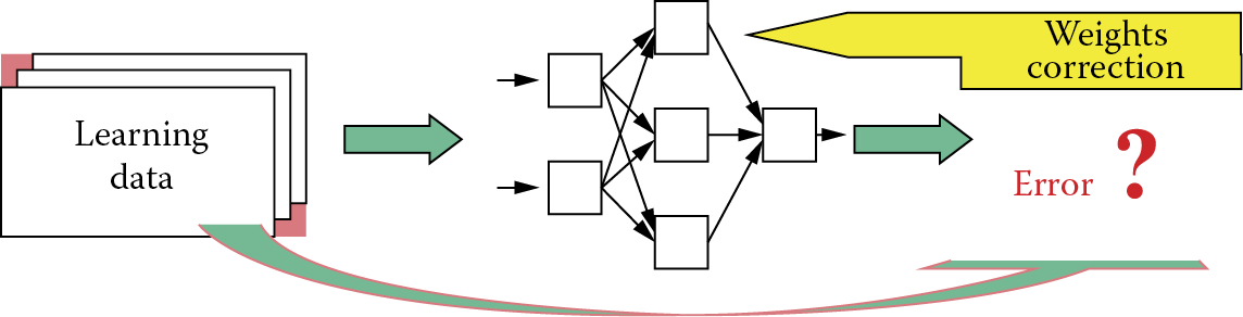
You will learn about the details of this process in later chapters. In simple terms, one teaches a network by providing it with input signals for which correct solutions are known because they are included in the learning data. For each given set of input data, the network tries to offer an output solution. Generally, the network’s suggestions differ from correct solutions included in the teaching data. After comparing the network solution with the correct exemplar solution in the teaching data, the extent of the error made by the network becomes clear. On the basis of mistake evaluation, the network’s teaching algorithm changes the weights of all its neurons so that the error will not be repeated in the future.
This simple model of a learning process indicates that a network tries to make no errors when presented with teaching data. Therefore, a network that learns well seeks a rule for processing input signals that would allow it to derive correct solutions. When a network discovers this rule, it can perform tasks from the teaching data it receives and similar tasks that may be assigned. We consider a successful network one that demonstrates an ability to learn and generalize learning results.
Unfortunately, a network that is too intelligent (has excessive memory in the form of large numbers of hidden neurons together with their adjustable weight sets) can easily avoid mistakes during learning by memorizing a whole collection of teaching data. It then achieves great success in learning within an astonishingly short time because it gives correct answers for all questions. However, in this method of “photographing” teaching data, a network that learns from provided examples of correct solutions makes no attempt at generalizing acquired information. Instead, it tries to achieve success by meticulously memorizing rules like “this input implies this output.”
Such incorrect operation of a network becomes obvious when the network quickly and thoroughly learns an entire teaching sequence (set of examples that demonstrate how it should perform assigned tasks) but fails embarrassingly in its first attempt to handle a task from similar class but slightly different from the tasks presented during learning. Teaching a network to recognize letters yields immediate success because it recognizes all letters shown. However, it will fail completely to recognize a letter in a different handwriting or font (all outputs are zero) or recognize them incorrectly. In such cases, an examination of the network’s knowledge reveals that it memorized many simple rules like “if two pixels are lit and there are five 0s, letter A should be recognized.” Such crude rules do not stand the test of a new task, and networks utilizing them fall short of expectations.
The described symptom of learning by memorizing is not displayed by networks with smaller hidden layers because limited memory forces a network to do its best. By using the few elements of its hidden layer, it works out rules for processing input signals that enable it to generate the required answer. In such cases, the learning process is usually considerably slower and more tedious because the network needs more examples presented more times—a few hundred or a few thousand. However, the final effect is usually much better. After a correctly conducted learning process is complete and a network effectively handles base learning examples, we may assume that it will also cope with similar (not identical) tasks presented during a test. The assumption is often (but not always) true and serves as a base for our expectations for using a network to solve problems.
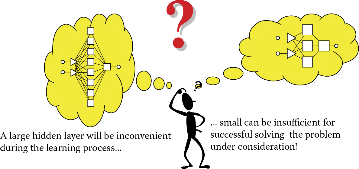
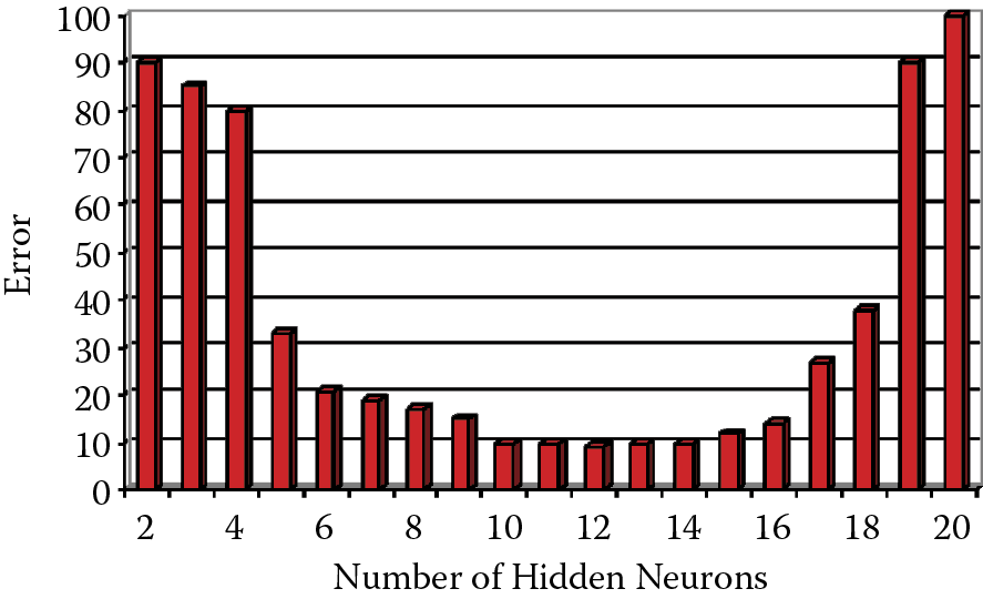
In summary, do not expect miracles. The presumption that an uncomplicated network with a few hidden neurons will succeed in a complicated task is unrealistic. Conversely, too many hidden layers or too many neurons can cause a significant decline in learning. Obviously, the optimal requirements for hidden layers lie somewhere between these extremes.
Figure 2.42 shows (on the basis of computer simulations) the relationship of network errors and numbers of hidden neurons. It proves that many networks operate with almost the same efficiency despite different numbers of hidden neurons. Thus it is not so difficult to hit such a broad target. Nevertheless, we must avoid extreme (too large or too small) networks. Especially undesirable are excessive) hidden layers. It is not surprising that networks with fewer hidden layers often produce better results. This is because they can be taught more effectively than better (theoretically) networks with more hidden layers where teaching is buried in unneeded details. The best practice in most situations is to use networks with one or (only as an exception) two hidden layers, and fight the temptation to use networks with more hidden layers—by fasting and taking cold baths!
References
Gee, A.H., and Prager, R.W. 1995. Limitations of neural networks for solving traveling salesman problems, IEEE Trans. Neural Networks, vol. 6, pp. 280–282.
Goddard, N., Hood, G., Howell, F., Hines, M., and De Schutter, E. 2001. NEOSIM: Portable large-scale plug and play modelling. Journal of Neurocomputing, vol. 38, pp. 1657–1661.
Hamill, O.P., Marty, A., Neher, E., Sakmann, B., and Sigworth, F.J. 1981. Improved patch-clump techniques for high-resolution current recording from cells and cell-free membrane patches. Pflugers Archive European Journal of Physiology, vol. 391 (2), pp. 85–100.
Hodgkin, A.L., and Huxley, A.F. 1952. A quantitative description of ion currents and its application to conduction and excitation in nerve membranes. Journal of Physiology, London, vol. 117, pp. 500–544.
Hopfield, J.J. 1982. Neural networks and physical systems with emergent collective computational abilities. Proc. of National Academy Scientific, USA, vol. 79, pp. 2554–2558.
Hopfield, J.J. 1985. Neural computation of decisions in optimizing problems. Biological Cybernetics, vol. 52, pp. 141–152.
Hopfield, J.J., and Tank, D.W. 1985. “Neural” computation of decisions in optimization problems, Biol. Cybern: vol. 52, pp. 141–152.
Rosenblatt, F. 1958. The Perceptron: A probabilistic model for information storage and organization in the brain. Psychological Review, American Psychological Association, vol. 65, No. 6, pp. 386–408.
Tadeusiewicz, R. and Figura I. 2011. Phenomenon of tolerance to damage in artificial neural networks. Computer Methods in Material Science, 11, 501–513.
Wang, H., Zhang, N., and Creput, J.-C. 2013. A massive parallel cellular GPU implementation of neural network to large-scale Euclidean TSP. Proc. 12th Mexican International Conference on Artificial Intelligence, MICAI 2013, LNCS vol. 8266, pp. 118–129.
Questions and Self-Study Tasks
1. What are some of the most significant differences between artificial neural networks and natural biological structures such as human and animal brains? Which differences result from capitulation (inability to build enough complicated artificial neurons and settling for substitutes)? Which differences are results of conscious deliberate choices by neural network creators?
2. Discuss the concept of synaptic weight, taking into account its role in artificial neural networks and also its biological inspiration. In electronic circuit modeling, neural networks weights are sometimes discrete (can only take certain values, e.g., integers) rather than arbitrary. How do you think weight exerts an impact on neural network functioning?
3. Introduce an artificial neuron scheme to transform input information into output signals. Demonstrate the differences between these transformation processes in particular types of neurons (linear, MLP, RBF).
4. Discuss the step-by-step operation of an artificial neural network. Why are hidden layers so named?
5. Discuss reactions between neural network structures and the functions the networks perform. Which are most popular neural network structures and what are their properties? Explain the ability of a randomly structured network to perform serious computational tasks.
6. What do you think about the ability of neural networks to show great fault tolerance when they encounter damages to the elements and destruction of their whole structures?
7. Why do neural networks require differentiation of quantitative and qualitative data? There is an opinion that networks that use qualitative data as inputs or outputs need more time for learning because they include more connections for which weights must be established. Is this opinion justified?
8. A network whose output data is encoded via the one of N method may not provide precise answers to questions. What could be the result? Should the lack of precision be seen as an advantage or a disadvantage?
9. Can time series analysis and related forecast tasks (see Figure 2.36) be considered more similar to regression tasks (Figure 2.34) or classification tasks (Figure 2.35)? What are the arguments for similarity to (a) regression and (b) classification?
10. Do Figure 2.37 and the text related to it lead to the conclusion that the application of a single network with many outputs is always ineffective? Specifically, if we must solve a problem whose expected output is in the form of qualitative data encoded by the one of N method, may we use N networks with one output each instead of one network with N outputs?
11. Advanced exercise: Assume you want to solve a certain classification with a neural network utilizing input data of questionability applicability and have doubts that the data will yield valuable information in the context of the classification under consideration. The issue is whether to use the doubtful input in a neural network because it could turn out to be useless. You could build your network without using a decision rule for the questionable data, or perhaps it would be better not to mix data to solve task variables that may be worthless. What is your choice? Justify your answer.
12. Advanced exercise: Books and articles describing neural networks sometimes propose the use of a genetic computer algorithm that somewhat simulates natural biological evolution. During evolution, the “fittest” network (having the best capabilities to produce a superior solution) will survive. The algorithm method can be used to select the best inputs for a network, estimate an optimal number of hidden layers, and evaluate the best hidden neurons in each layer. Study more about this method and develop an opinion whether it is or is not effective. Present arguments for both positions.