
![]()
Analysis of Variance
So far, we have explored hypothesis tests that cope with at most two samples. Now, of course, they could be run multiple times—it would be trivial to extend loops and t.test to run through many iterations. However, that is a proposition fraught with risk. For a given = 0.05, suppose we wish to compare mean staph infection rates for eight regional medical centers. Then there are choose(8,2) = 28 total pairwise comparisons. Thus, the chance of at least one Type I error, supposing our eight samples are independent, is 1 – (.95)28 = 0.7621731 which is rather high. Analysis of variance (ANOVA) compares three or more means simultaneously, thereby controlling the error rate to the nominal 0.05.
Regardless of the precise type, ANOVA is built on the underlying premise that the variance between our samples (e.g., the sample means) may be compared with sample variance within our samples to determine if it seems reasonable that there is a significant difference between means. An F-ratio is built where the between variances are divided by the within variances. Suppose we have a rather large difference between some of our sample means. This would lead us to suspect at least one of those regional medical centers has an overly high rate of staph infection incidents. However, suppose that the sample standard deviations tend to be rather large—that sort of numerical turbulence would lead us to revise our first-blush instinct toward believing that despite the difference in means, perhaps the centers are all essentially similar. The closer this F-ratio is to one, the more support there is for the null hypothesis vis-à-vis sample size(s). Generally, a p value is calculated for the F-distribution for NHST (null hypothesis significance testing). As we delve into particulars, we caution our readers that the more complex the ANOVA methodology, the more care required in results interpretation.
In this chapter, we will compare the means of three or more groups with one-way ANOVA, followed by the post-hoc comparisons of the Tukey HSD (honest significant difference) criterion. Then, we will delve further into two-way ANOVA, repeated-measures ANOVA, and mixed-model ANOVA.
We leave mathematical explorations of ANOVA to other texts. However, it is essential to know the three requirements for ANOVA methods to hold true. We suppose the samples are random and independent (although we show how to relax this assumption in repeated-measures ANOVA). We also suppose that the populations from which we draw the samples are both normal and have the same variance. The latter two requirements are generally somewhat relaxed, and ANOVA may give practical guidance even in scenarios where the populations are not quite normal or where the variances do not quite match, particularly as long as the distributions are at least symmetrical. More precise definitions of “quite” are controversial and any specific threshold may be misleading in particular cases. If there is concern about whether the assumptions for an ANOVA are met, one approach is to try another test that does not have the same assumptions (e.g., non-parametric tests) to see whether or not the same conclusions are reached using both approaches. Where there are k groups, the default null hypothesis for ANOVA is H0: μ1 = … = μk.
With three or more independent samples, we extend the independent-samples t-test to the one-way ANOVA. The paired-samples t-test is also extended to the repeated-measures ANOVA, in which each observation has three or more repeated measures on the same dependent variable.
Using simulated student final score data (to not run afoul of confidentiality laws), let us suppose our data were randomly drawn and independent (we acknowledge that random draws from education data may be difficult if not impossible/unethical). The alternative hypothesis is that at least one mean is different. Certainly the means in the latter terms look higher (see Figure 12-1). Note that we use the factor() function in order to relevel the factor and enforce chronological order.
> myData <- read.table("ANOVA001.txt", sep="	", header=TRUE)
> myData$Term <- factor(myData$Term, levels = c("FA12", "SP13", "FA13"))
> plot(Score ~ Term, data=myData)

Figure 12-1. Box-and-whisker plots of the score data for each term
For an ANOVA run to be legitimate, our data are required to be drawn from normal populations. Visual inspection of the graphs may be a good first place to start (most introductory statistical methods courses often either simply assume normality or simply “eyeball” it). A glance at the histograms in this case may be inconclusive (see Figure 12-2). Notice how we can add color to the histograms depending on which term they are from and also make three separate plots via faceting using facet_wrap() and specifying the variable to facet, in our case by Term. Finally, since we made separate plots by term in addition to adding color, we turn off the automatic legend (by specifying an option to the theme() function) that would be created for color, as that is redundant with the individual plots.
> library ( gridExtra )
> library ( ggplot2 )

> ggplot(myData, aes(Score, color = Term)) +
+   geom_histogram(fill = "white", binwidth = 10) +
+   facet_wrap(~ Term) +
+   theme(legend.position = "none")

Figure 12-2. Histograms of the various scores by term looking somewhat normal
Numerical methods are often preferred to graphical methods. Empirical tests by Razali and Wah (2011) suggest the Shapiro-Wilk (SW) normality test on each level or factor of our data. By using for(), we make the code much cleaner and avoid repeated typing as well as the associated chance for error(s).
> for (n in levels(myData$Term)) {
+   test <- with(subset(myData, Term == n), shapiro.test(Score))
+   if (test$p.value < 0.05) {
+     print(c(n, test$p.value))
+   }
+ }
As our loop printed no values, we continue to check whether the variances are the same for each sample. The Bartlett test for homogeneity of variances (also called homoscedasticity) is built into R. Bartlett's test is often considered to be sensitive to normality. Since ANOVA requires normality, this is not of particular concern. Levene's Test is another popular test of homoscedasticity, although it would require installing another package.
> bartlett.test(Score ~ Term, data = myData)

        Bartlett test of homogeneity of variances

data:  Score by Term
Bartlett's K-squared = 1.199, df = 2, p-value = 0.5491
We do not reject the null hypothesis and, having verified or supposed the requirements of one-way ANOVA, may proceed. We run an ANOVA in R using the aov() function and then create a summary of that model using the summary() function. We see that the scores by term are statistically significantly different with a standard alpha of 0.05.
> results <- aov(Score ~ Term, data = myData)
> summary(results)
Analysis of Variance Table

Response: Score
          Df Sum Sq Mean Sq F value  Pr(>F)
Term       2 1123.4  561.69  3.2528 0.04622 *
Residuals 55 9497.3  172.68
---
Signif. codes:  0 '***' 0.001 '**' 0.01 '*' 0.05 '.' 0.1 ' ' 1
The command TukeyHSD() calculates the HSDs and is often used as a post-hoc test after ANOVA (when the null hypothesis is rejected). This allows us to see (or perhaps confirm in this case) that the only difference trending toward statistical significance is the FA12 to FA13. Supposing our treatment had begun in SP13, we may need further study before concluding our course modifications a success! In addition to displaying the mean difference between specific pairwise contrasts (FA13 - FA12), we also see the 95% confidence interval, shown as the lower (lwr) and upper (upr) bounds.
> TukeyHSD(results)
  Tukey multiple comparisons of means
    95% family-wise confidence level

Fit: aov(formula = Score ~ Term, data = myData)

$Term
               diff         lwr      upr     p adj
SP13-FA12  8.129921 -2.01040487 18.27025 0.1395847
FA13-FA12 10.086237 -0.05408909 20.22656 0.0515202
FA13-SP13  1.956316 -8.31319147 12.22582 0.8906649
One-way ANOVA can be extended to a two-way ANOVA by the addition of a second factor, and even higher-order ANOVA designs are possible. We can also use mixed-model ANOVA designs in which one or more factors are within subjects (repeated measures). We explore these more in the next section.
With the two-way ANOVA, we have two between-groups factors, and we test for both main effects for each factor and the possible interaction of the two factors in their effect on the dependent variable. As before, the requirements of normal populations and the same variance hold, and while these should be checked, we suppress those checks in the interest of space. This time, we build a model using data from the MASS package, and use both SES (socioeconomic status) and a language test score as factors to study verbal IQ. We use a completely crossed model and test for main effects as well as interaction. We see significant main effects for both factors but a nonsignificant interaction, as displayed in the ANOVA summary table.
> library(MASS)
> twoway <- aov(IQ ~ SES * lang, data = nlschools)
> summary ( twoway )
              Df Sum Sq Mean Sq  F value Pr(>F)
SES            1    982   981.9  372.018 <2e-16 ***
lang           1   2769  2769.1 1049.121 <2e-16 ***
SES:lang       1      8     8.1    3.051 0.0808 .
Residuals   2283   6026     2.6
---
Signif. codes:  0 '***' 0.001 '**' 0.01 '*' 0.05 '.' 0.1 ' ' 1
Since the interaction of SES x lang is not significant, we may want to drop it and examine the model with just the two main effects of SES and lang. We could write out the model formula again and rerun it, but we can also update existing models to add or drop terms. It does not make much difference with a simple model as shown in this example, but with more complex models that have many terms, rewriting all of them can be tedious and complicate the code. In the formula, the dots expand to everything, so we update our first model by including everything on the left-hand side of the ~ and everything on the right-hand side, and then subtracting the single term we want to remove, SES x lang. If we had wanted to add a term, we could do that to using + instead of -.
> twoway.reduced <- update(twoway, . ~ . - SES:lang)
> summary ( twoway.reduced )
              Df Sum Sq Mean Sq F value Pr(>F)
SES            1    982   981.9   371.7 <2e-16 ***
lang           1   2769  2769.1  1048.2 <2e-16 ***
Residuals   2284   6034     2.6
---
Signif. codes:  0 '***' 0.001 '**' 0.01 '*' 0.05 '.' 0.1 ' ' 1
In this case, removing the interaction made little difference and we draw the same conclusions that both SES and language are still significant.
12.3.1 Repeated-Measures ANOVA
The one-way repeated-measures ANOVA is a special case of the two-way ANOVA with three or more measures for the same subjects on the same dependent variable. Suppose we measured fitness level on a scale of 0 to 10 for six research subjects who are participating in a supervised residential fitness and weight loss program. The measures are taken on the same day and time and under the same conditions for all subjects every week. The first four weeks of data are as shown below. Note that we must explicitly define the subject id and the time as factors for our analysis. To convert some of the variables to factors within the data frame, we use the within() function, which tells R that everything we do within the curly braces should be done within the data frame referenced.
> repeated <- read.table("repeated_fitness_Ch12.txt", sep = " ", header = TRUE)
> repeated
   id time fitness
1   1    1       0
2   1    2       1
3   1    3       3
4   1    4       4
5   2    1       1
6   2    2       2
7   2    3       4
8   2    4       5
9   3    1       2
10  3    2       3
11  3    3       3
12  3    4       5
13  4    1       3
14  4    2       4
15  4    3       4
16  4    4       5
17  5    1       2
18  5    2       3
19  5    3       3
20  5    4       4
21  6    1       2
22  6    2       3
23  6    3       3
24  6    4       5


> repeated <- within(repeated, {
+   id <- factor ( id )
+   time <- factor ( time )
+ })
> results <- aov ( fitness ~ time + Error (id / time ), data = repeated)
> summary ( results )

Error: id
          Df Sum Sq Mean Sq F value Pr(>F)
Residuals  5  8.333   1.667

Error: id:time
          Df Sum Sq Mean Sq F value   Pr(>F)
time       3   28.5   9.500    28.5 1.93e-06 ***
Residuals 15    5.0   0.333
---
Signif. codes:  0 '***' 0.001 '**' 0.01 '*' 0.05 '.' 0.1 ' ' 1
We see that the effect of time is significant. A means plot makes this clearer (see Figure 12-3). We use the ggplot2 stat_summary() function to calculate the means for the six subjects for each week and to plot both points and lines. Note that since we converted time into a factor before, but here we want to use it as a numerical variable for the x axis, we convert back to a number using the as.numeric() function.
> library(ggplot2)
> meansPlot <- ggplot(repeated, aes (as.numeric(time) , fitness)) +
+   stat_summary(fun.y = mean , geom ="point") +
+   stat_summary (fun.y = mean , geom = "line")
> meansPlot

Figure 12-3. Means plot for fitness over time
stat_summary() function, using a different summary function and the point-range geom rather than just points (see Figure 12-4).
> meansPlot2 <- ggplot(repeated, aes (as.numeric(time) , fitness)) +
+   stat_summary(fun.data = mean_cl_normal, geom ="pointrange") +
+   stat_summary (fun.y = mean , geom = "line")
> meansPlot2

Figure 12-4. Means plot with 95% confidence intervals for fitness over time
A mixed-model ANOVA, as mentioned earlier, must have at least one within-subjects (repeated-measures) factor, and at least one between-groups factor. Let’s take a simple example, that of a design in which groups of older and younger adults are taught a list of 20 five-letter words until they can recall the list with 100% accuracy. After learning the list, each subject attempts to recall the words from the list by listening to the target words and 20 additional five-letter distractor words randomly chosen by a computer under three different conditions: no distraction (the subject listens with eyes closed and pushes a button if he or she recognizes the word as being on the list), simple distraction (the subject performs the same task with open eyes and background music), or complex distraction (the subject performs the same task while engaged in a conversation with the experimenter). The data are as follows. We read the data from a CSV file and allow R to assign the string variables to factors (the default):
> mixedModel <- read.csv("mixedModel.csv")
> str ( mixedModel )
'data.frame':   24 obs. of  4 variables:
 $ id   : Factor w/ 8 levels "A","B","C","D",..: 1 1 1 2 2 2 3 3 3 4 ...
 $ age  : Factor w/ 2 levels "old","young": 2 2 2 2 2 2 2 2 2 2 ...
 $ distr: Factor w/ 3 levels "h","l","m": 2 3 1 2 3 1 2 3 1 2 ...
 $ score: int  8 5 3 7 6 6 8 7 6 7 ...
> mixedModel
   id   age distr score
1   A young     l     8
2   A young     m     5
3   A young     h     3
4   B young     l     7
5   B young     m     6
6   B young     h     6
7   C young     l     8
8   C young     m     7
9   C young     h     6
10  D young     l     7
11  D young     m     5
12  D young     h     4
13  E   old     l     6
14  E   old     m     5
15  E   old     h     2
16  F   old     l     5
17  F   old     m     5
18  F   old     h     4
19  G   old     l     5
20  G   old     m     4
21  G   old     h     3
22  H   old     l     6
23  H   old     m     3
24  H   old     h     2
The ez package makes it easier to perform ANOVA for a variety of designs, including the mixed-model ANOVA. We will use the ezANOVA() function, which will also perform the traditional test of the sphericity assumption, along with appropriate corrections if sphericity cannot be assumed, after producing the standard ANOVA summary table. The table lists the specific effect, followed by the numerator and denominator degrees of freedom for each test, the F value, p value, and stars if the p value is less than .05. One other useful output, labeled “ges,” is the generalized h2, a measure of the size or magnitude of each effect, beyond its statistical significance.
> install.packages ("ez")
> library (ez)
> ezANOVA ( mixedModel , score , id , distr , between = age )
$ANOVA
     Effect DFn DFd          F           p p<.05        ges
2       age   1   6 15.7826087 0.007343975     * 0.54260090
3     distr   2  12 19.5000000 0.000169694     * 0.64084507
4 age:distr   2  12  0.2142857 0.810140233       0.01923077

$`Mauchly's Test for Sphericity`
     Effect         W         p p<.05
3     distr 0.5395408 0.2138261
4 age:distr 0.5395408 0.2138261

$`Sphericity Corrections`
     Effect       GGe       p[GG] p[GG]<.05       HFe        p[HF] p[HF]<.05
3     distr 0.6847162 0.001321516         * 0.8191249 0.0005484227         *
4 age:distr 0.6847162 0.729793578           0.8191249 0.7686615724
We see that we have significant effects for the age and distraction condition, but no significant interaction. Mauchly's test for sphericity is not significant, suggesting that the results meet the sphericity assumption for mixed-model ANOVAs, and we can also see that the p values corrected for the (nonsignificant) lack of sphericity, labeled p[GG] and p[HF] for the Greenhouse-Geisser correction and Huynh-Feldt correction, respectively, are essentially the same as in the uncorrected ANOVA summary table. An interaction plot, which is quite easy to produce using the base R graphics package, shows the nature of these effects (see Figure 12-5). We can use the with() function to reference the three variables from within the mixedModel data frame, without typing its name each time. The plot (Figure 12-5) shows that younger adults have better recall than older adults at all three levels of distraction, and the fact that all three lines are virtually parallel agrees with the nonsignificant interaction found from the ANOVA.
> with(mixedModel, interaction.plot (age , distr , score ))
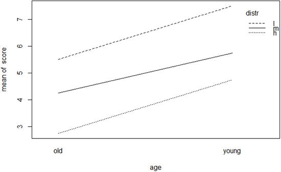
Figure 12-5. Interaction plot for age and distraction condition
References
Razali, N. M., & Wah, Y. B. “Power comparisons of Shapiro-Wilk, Kolmogorov-Smirnov, Lilliefors and Anderson-Darling tests.” Journal of Statistical Modeling and Analytics, 2(1), 21-33 (2011).