Tables are very useful for summarizing data. We can use tables for all kinds of data, ranging from nominal to ratio. In Chapter 7, you will learn how to use tables to create frequency distributions and cross-tabulations as well as how to conduct chi-square tests to determine whether the frequencies are distributed according to some null hypothesis.

The table() function in R returns a contingency table, which is an object of class table, an array of integer values indicating the frequency of observations in each cell of the table. For a single vector, this will produce a simple frequency distribution. For two or more variables, we can have rows and columns, the most common of which will be a two-way contingency table. We can also have higher-order tables. For example, the HairEyeColor data included with R are in the form of a three-way table, as we see in the following code:

> data(HairEyeColor)
> HairEyeColor
, , Sex = Male
        Eye
Hair    Brown Blue Hazel Green
Black    32   11    10     3
Brown    53   50    25    15
Red      10   10     7     7
Blond     3   30     5     8
, , Sex = Female

        Eye
Hair    Brown Blue Hazel Green
Black    36    9     5     2
Brown    66   34    29    14
Red      16    7     7     7
Blond     4   64     5     8

> class(HairEyeColor)
[1] "table"

7.1 Working with One-Way Tables

For those who are not familiar with the terminology of a “one-way” table, it is a listing of the possible values for the variable being summarized and an adjacent list of the frequency of occurrence for each of the values. A table can summarize the counts for anything that can be considered or interpreted as a factor, and we can build tables from both raw data and summary data. For example, in an analysis we might perform on the hsb data we met in Chapter 3, I created categories for the math variable so they could be used as an ordinal factor. Figure 7-1 shows the original data.

The cut2 function in the Hmisc package makes it easy to create the new variable, and the table function shows that the groups are indeed roughly equal in size. Through a bit of experimentation, I found that a good choice was five math groups (I rather thought of the five American letter grades of ABCDF). I assigned an integer to represent each group by adding the as.numeric function. The g argument specifies the number of groups. Note that if you do not use a convenient label for the group membership, the cut2 function will provide the interval limits as labels.

> hsb <- read.csv ("http://www.ats.ucla.edu/stat/data/hsb.csv")
> install.packages("Hmisc")
> library(Hmisc)

> hsb$mathGp <- as.numeric(cut2(hsb$math, g = 5))
> head(hsb)
   id female race ses schtyp prog read write math science socst mathGp
1  70      0    4   1      1    1   57    52   41      47    57      1
2 121      1    4   2      1    3   68    59   53      63    61      3
3  86      0    4   3      1    1   44    33   54      58    31      3
4 141      0    4   3      1    3   63    44   47      53    56      2
5 172      0    4   2      1    2   47    52   57      53    61      4
6 113      0    4   2      1    2   44    52   51      63    61      3

> table(hsb$math)

33 35 37 38 39 40 41 42 43 44 45 46 47 48 49 50 51 52 53 54 55 56 57 58 59 60 61 62
 1  1  1  2  6 10  7  7  7  4  8  8  3  5 10  7  8  6  7 10  5  7 13  6  2  5  7  4
63 64 65 66 67 68 69 70 71 72 73 75
 5  5  3  4  2  1  2  1  4  3  1  2

> hsb$mathGp2 <- cut2(hsb$math, g = 5)
> head(hsb)
   id female race ses schtyp prog read write math science socst mathGp mathGp2
1  70      0    4   1      1    1   57    52   41      47    57      1 [33,44)
2 121      1    4   2      1    3   68    59   53      63    61      3 [50,56)
3  86      0    4   3      1    1   44    33   54      58    31      3 [50,56)
4 141      0    4   3      1    3   63    44   47      53    56      2 [44,50)
5 172      0    4   2      1    2   47    52   57      53    61      4 [56,62)
6 113      0    4   2      1    2   44    52   51      63    61      3 [50,56)

> table(hsb$mathGp2)

[33,44) [44,50) [50,56) [56,62) [62,75]
     42      38      43      40      37

Let’s examine a table of the frequencies of the three different SES (socioeconomic status) levels in the hsb data. These vary substantially from level to level.

> table(hsb$ses)

 1  2  3
47 95 58

When we have observed frequencies in two or more categories, as in this example, we can perform a chi-square test of goodness of fit comparing the observed frequencies with the expected frequencies if each category had an equal number of observations. We can also test to see if an observed frequency distribution matches a theoretical one when the expected frequencies are not equal. With a total of k categories, the value of chi square is calculated as:

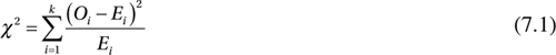
where O is the observed frequency in each cell and E is the expected frequency for that cell under the null hypothesis that the observed and expected frequencies are equal. As the deviations between the observed and expected frequencies become larger in absolute value, the value of chi square increases, and if the p value is lower than our specified alpha level, we reject the null hypothesis. Let’s test to see if the SES levels are evenly distributed, adopting an alpha level of .01.

> chisq.test(table(hsb$ses))

        Chi-squared test for given probabilities

data:  table(hsb$ses)
X-squared = 18.97, df = 2, p-value = 7.598e-05

We reject the null hypothesis. Clearly, SES is distributed unequally. Note the degrees of freedom are the number of categories minus one. As indicated earlier, there is no particular reason the expected cell frequencies must be uniformly distributed. Chi-square tests of goodness of fit can be used to determine whether an observed frequency distribution departs significantly from a given theoretical distribution. The theoretical distribution could be uniform, but it might also be normal or some other shape.

We can use summary data in addition to tables for chi-square tests. For example, suppose we find that in a sample of 32 automobiles, there are 11 four-cylinder vehicles, 7 six-cylinder vehicles, and 14 eight-cylinder vehicles. We can create a vector with these numbers and use the chi-square test as before to determine if the number of cylinders is equally distributed.

> cylinders <- c(7, 11, 14)
> names(cylinders) <- c("four", "six", "eight")
> cylinders
four   six eight
   7    11    14
> chisq.test(cylinders)

Chi-squared test for given probabilities

data:  cylinders
X-squared = 2.3125, df = 2, p-value = 0.3147

The degrees of freedom, again, are based on the number of categories, not the sample size, but the sample size is still important. With larger samples, the deviations from expectation may be larger, making the chi-square test more powerful.

When the expected values are unequal, we must provide a vector of expected proportions under the null hypothesis in addition to observed values. Assume we took a random sample of 500 people in a given city and found their blood types to be distributed in the fashion shown in in Table 7-1. The expected proportions are based on the U.S. population values.

Let us test the null hypothesis that the blood types in our city are distributed in accordance with those in the U.S. population using an alpha level of .05. Here is the chi-square test. Note we receive a warning that the value of chi square may be incorrect due to the low expected value in one cell.

> obs <- c(195, 165, 47, 15, 30, 35, 8, 5)
> exp <- c(0.374, 0.357, 0.085, 0.034, 0.066, 0.063, 0.015, 0.006)
> chisq.test(obs, p = exp)

Chi-squared test for given probabilities

data:    obs
X-squared = 4.1033, df = 7, p-value = 0.7678

Warning message:
In chisq.test(obs, p = exp) : Chi-squared approximation may be incorrect

On the basis of the p value of .768, we do not reject the null hypothesis, and we conclude that the blood types in our city are distributed in accordance with those in the population.

7.2 Working with Two-Way Tables

With two-way tables, we have r rows and c columns. To test the null hypothesis that the row and column categories are independent, we can calculate the value of chi square as follows:

The expected values under independence are calculated by multiplying each cell’s marginal (row and column) totals and dividing their product by the overall number of observations. As with one-way tables, we can use the table function in R to summarize raw data or we can work with summaries we have already created or located.

The degrees of freedom for a chi-square test with two categorical variables is (r − 1)(c − 1). The chi-square test for a two-by-two table will thus have 1 degree of freedom. In this special case, we are using the binomial distribution as a special case of the multinomial distribution, and the binomial distribution is being used to approximate the normal distribution. Because the binomial distribution is discrete and the normal distribution is continuous, as we discussed earlier in Chapter 6, we find that a correction factor for continuity improves the accuracy of the chi-square test. By default, R uses the Yates correction for continuity for this purpose.

Assume we have information concerning the frequency of migraine headaches among a sample of 120 females and 120 males. According to the Migraine Research Foundation, these headaches affect about 18% of adult women and 6% of adult men. We have already been given the summary data, so we can use it to build our table and perform our chi-square test as follows. Let’s adopt the customary alpha level of .05.

> migraine <- matrix(c(19, 7, 101, 113), ncol = 2, byrow = TRUE)
> colnames(migraine) <- c("female", "male")
> rownames(migraine) <- c("migraine", "no migraine")
> migraine <- as.table(migraine)
> migraine
            female male
migraine        19    7
no migraine    101  113

> chisq.test(migraine)

Pearson's Chi-squared test with Yates' continuity correction

data:  migraine
X-squared = 5.2193, df = 1, p- value = 0.02234

As you see, we applied the Yates continuity correction. We reject the null hypothesis in favor of the alternative and conclude that there is an association between an adult’s sex and his or her frequency of being a migraine sufferer.

It is also possible easily to use the table function to summarize raw data. For example, here is a cross-tabulation of the sexes and SES groups of the students in the hsb dataset. The chi-square test will now have 2 degrees of freedom because we have two rows and three columns. Let us determine if the sexes of the students are associated with the SES level, which we would hope would not be the case.

table(hsb$female, hsb$ses)

     1  2  3
  0 15 47 29
  1 32 48 29
> femaleSES <- table(hsb$female, hsb$ses)
> chisq.test(femaleSES)

       Pearson's Chi-squared test

data:  femaleSES
X-squared = 4.5765, df = 2, p-value = 0.1014

I named the table just to reduce the clutter on the command line. As we see, we do not reject the null hypothesis, and we conclude the SES levels and student sex are independent.