
Now that we have a functioning Raspberry Pi sensor that includes the baseline recorder, sensor, and reports, let’s do an operational walk-through.
Raspberry Pi Setup
The first step is to set up the Raspberry Pi sensor.
- 1.
Raspberry Pi Model 3
- 2.
Minimum of 16GB SD card
- 3.
Install the Raspbian OS (this is the current version running)
PRETTY_NAME="Raspbian GNU/Linux 8 (jessie)"NAME="Raspbian GNU/Linux"VERSION_ID="8"VERSION="8 (jessie)"ID=raspbianID_LIKE=debian - 4.
Once you have this installed, update the Python 2.7 version to the latest, which currently is 2.7.9 or greater. Note this step is only necessary if you plan to work with the Python source code. The executable for piSensorV3 is also being provided with this book.
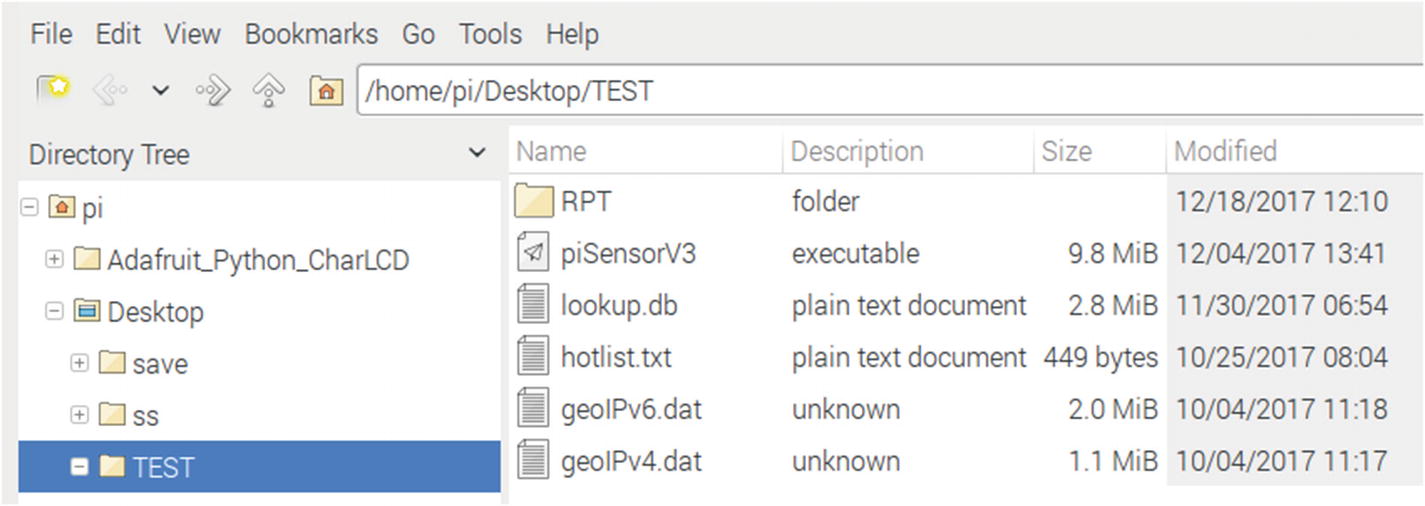
- 5.Copy installation files available at python-forensics.org/piSensor to a folder of your choice on the Pi. For my test installation, I placed the files in a folder named TEST right on the desktop of the Pi. Figure 5-1 depicts the contents of the folder TEST.
- a.
RPT Folder: Reports and baselines are written to this folder by the Raspberry Pi sensor
- b.
piSensorV3 is the compiled Python sensor application
- c.
lookup.db contains the various lookup tables for ports, protocols, MAC address manufacturers, and Ethernet types
- d.
The geoIPv6 and geoIPv4 files are used to map IP addresses to country locations
- e.
hotlist.txt contains a list of ports of interest
- a.
Operational folder
Optional Features:
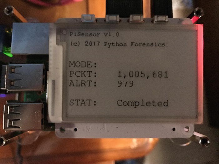
Raspberry Pi with PaPirus ePaper display
Connecting the Raspberry Pi
The next step is to connect the Raspberry Pi to the network you wish to monitor.
Switch Configuration for Packet Capture
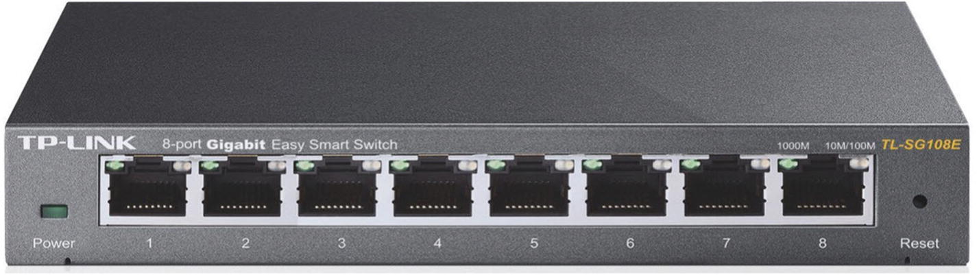
TP-LINK eight-port Gigabit Easy Smart Switch
The simplicity of the switch is based on the software application “Easy Smart Configuration Utility,” shown in Figure 5-4, that is included with the switch. The configuration utility allows for the configuration of all the features available on the TL-SG108E.
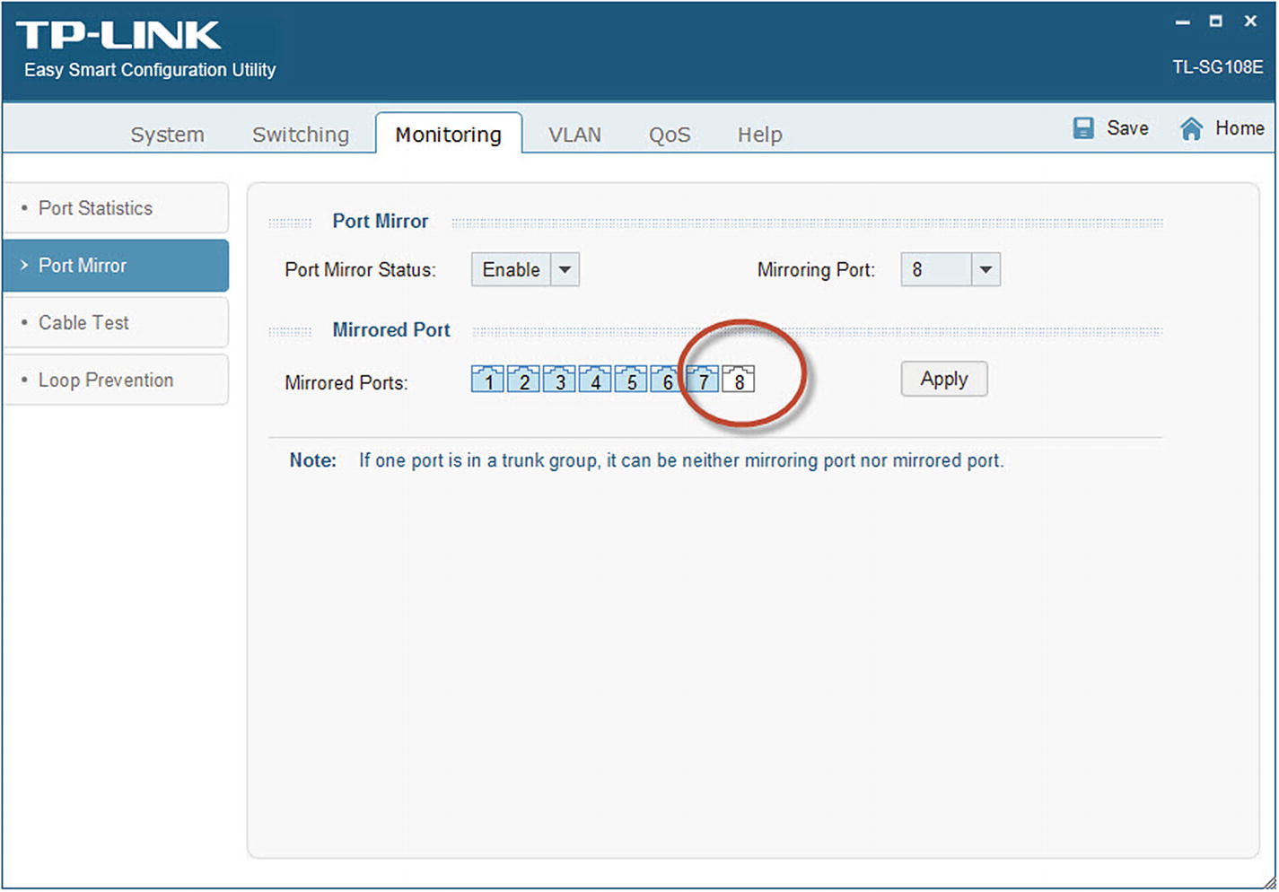
Easy Smart configuration utility
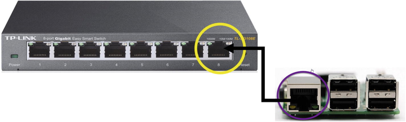
Connecting the Pi sensor to the TP-LINK monitoring port
Running the Python Application
- 1.
Why is this not just a Python file? You could of course launch the Python interpreter and specify the main Python script piSensorV3.py. You would need to download the Python scripts as noted in the Appendix A to do this. Note that piSensorV3.py is a Python 2.7 script and will not work in Python 3.x environments. However, the piSensorV3 application does not rely on the underlying Python installation.
sudo python piSensorV3.py - 2.
How did you make the Python script into an executable? There are several methods to convert Python scripts into more traditional executables. I have found that the pyinstaller is an outstanding product to convert Python scripts into executables. You can find more information about pyinstaller at the following website:
www.pyinstaller.org/
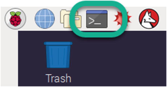
Open a terminal window
- 1.
Navigate to the folder where you copied the required files. On my Raspberry Pi, I navigated to the desktop, then to the TEST folder. I then typed “ls” to verify that the directory contained the required files.
- 2.
Launch the executable. Notice that I launched the executable from the current working directory, and I launched this as sudo. This is required since piSensorV3 requires privilege to place the network adapter in promiscuous mode.
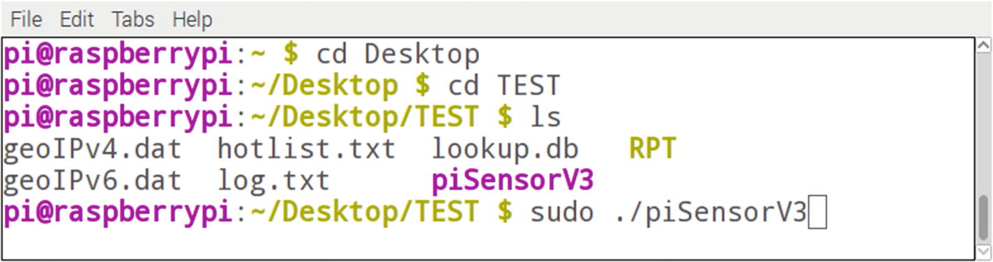
Terminal window execution of piSensorV3
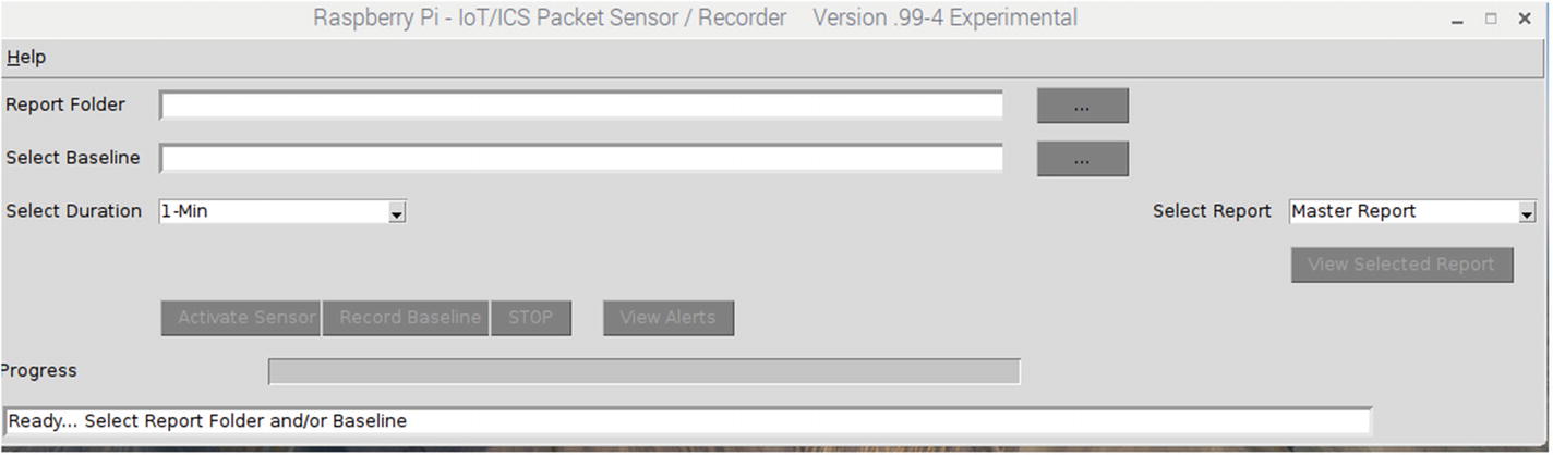
piSensorV3 application launched
Note
If you have a PaPirus display installed, the display will be initialized and display the initial prompts.
Creating a Baseline
The next step in the operation is to create a baseline of the network you are monitoring. This will be used by the sensor later to monitor device behaviors when in sensor mode. However, much can be gleaned about your network by recording the baseline as well.
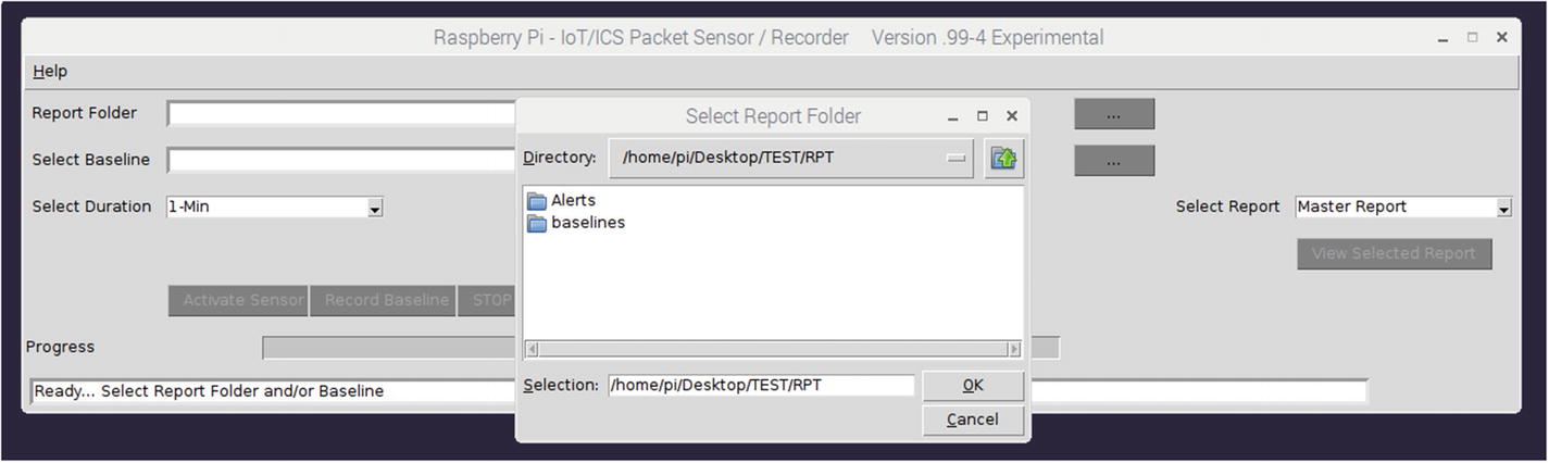
Report folder selection
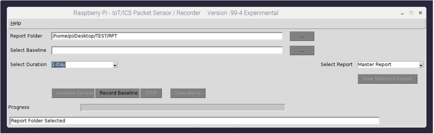
Report and duration selected
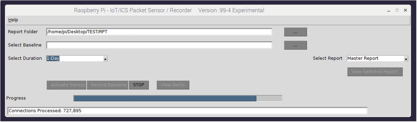
Baseline recording progress
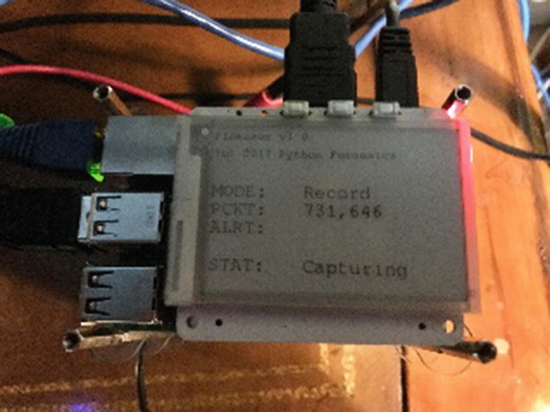
PaPirus recording progress display
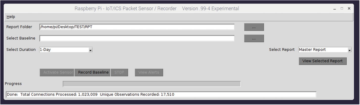
Baseline recording completed
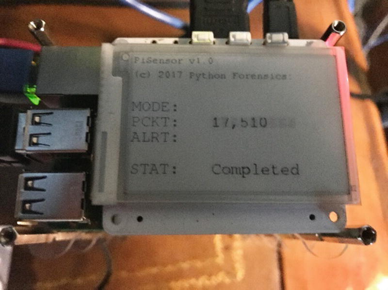
Baseline completed PaPirus display
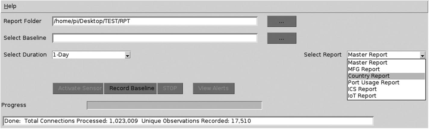
Report selection
- 1.Master - This report includes all recorded observations (in this example, 17,510 records) with details of each recording as shown in Figure 5-15. See the report excerpt in Figure 5-16 for an abbreviated example of the master report contents.
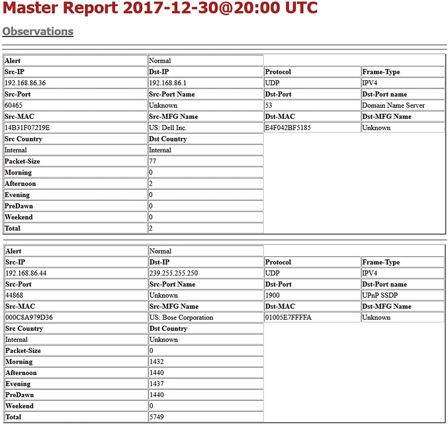 Figure 5-16
Master report excerpt
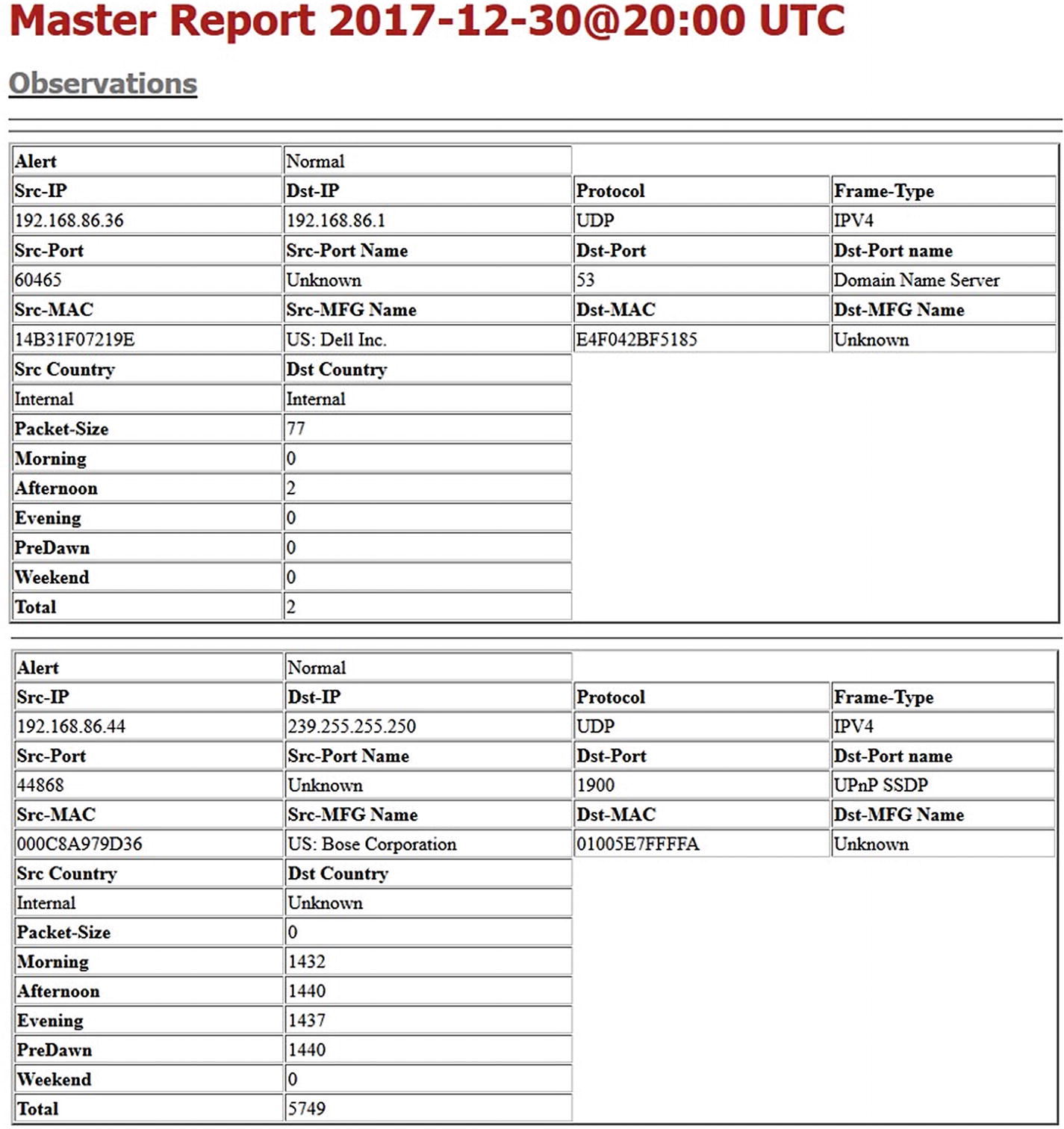 Figure 5-17
Master report excerpt continued
- 2.Device manufacturer report – This report provides observation of each device manufacturer along with the associated MAC and IP address. This provides detailed tracking of known and possibly unknown devices located on your network. During the sensor phase, any device that was not observed during the recording period is reported as an alert. See the report in Figure 5-18 for an abbreviated example.
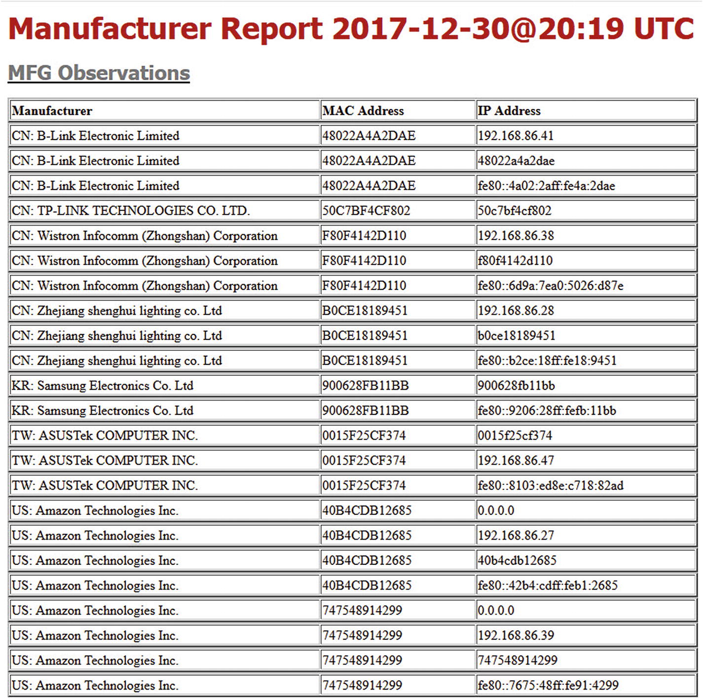 Figure 5-18
Excerpt of the manufacturer report
- 3.Country report - Much like the manufacturer report, the data is organized by observed country. Included in the report is the number of connections made to systems within the targeted country. Again, during the sensor phase, any country connections not observed during the recording period generate an alert. Figure 5-19 shows an example of the country report.
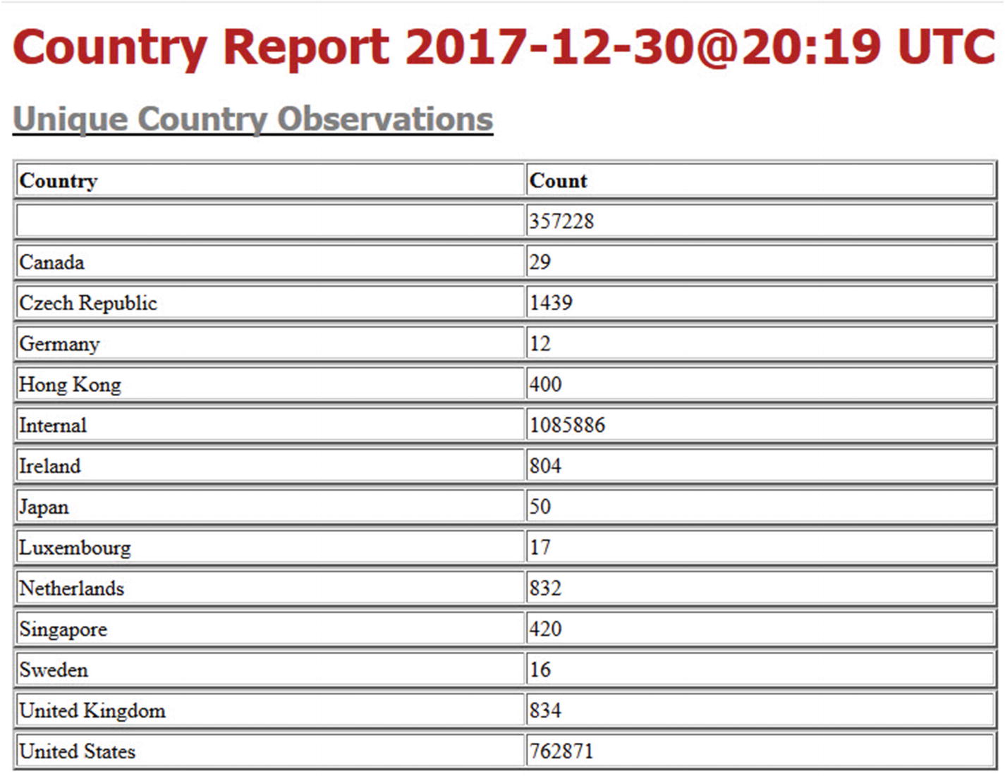 Figure 5-19
Report observed country connections
- 4.Port usage report – This report organizes the data by observed port connections. The report contains each used port number and associated name, along with the unique source and destination IP addresses, frame type, and associated protocol that was used. Figure 5-20 depicts an excerpt from the port usage report.
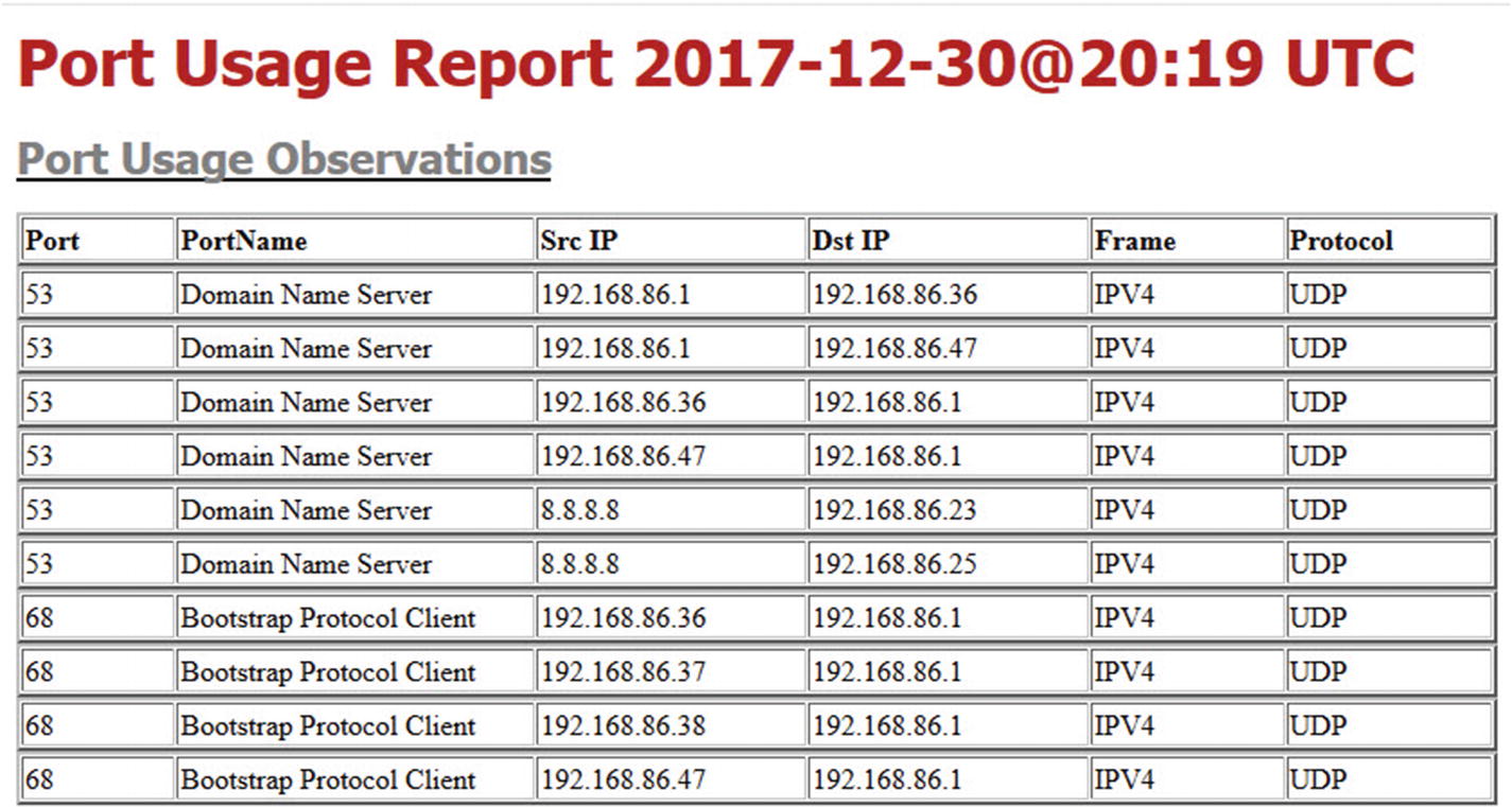 Figure 5-20
Port usage report
- 5.Known ICS port usage report and IoT port usage report – These reports further filter the port usage to the only ports that are typically utilized by ICS or IoT devices. It is important to note that some of the port reports can have non-ICS/IoT usage as well. Thus, the reports are named Possible ICS and Possible IoT Port Usage. Report Excerpts E and F provide samples of these reports. During sensor operation, any ICS or IoT observations that did not exist during the recording period will generate an alert. See Figures 5-21 and 5-22 for samples of the ICS and IoT reports.
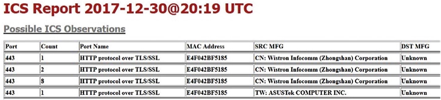 Figure 5-21
ICS report sample
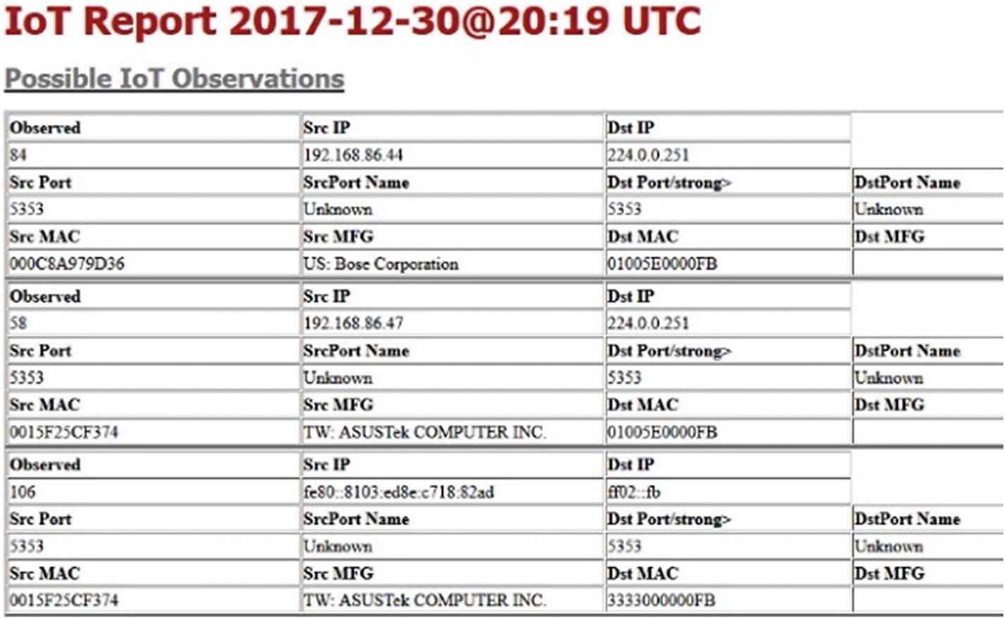 Figure 5-22
IoT report sample
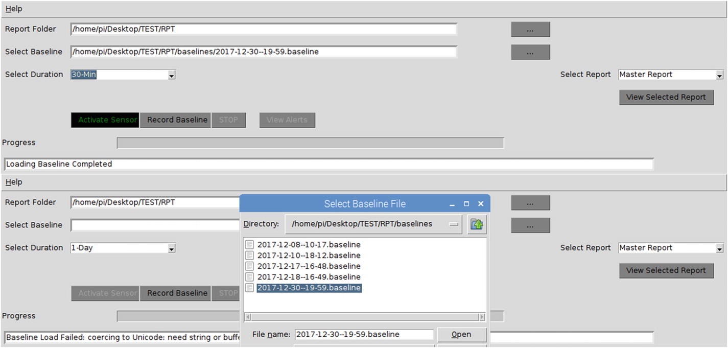
Baseline selection
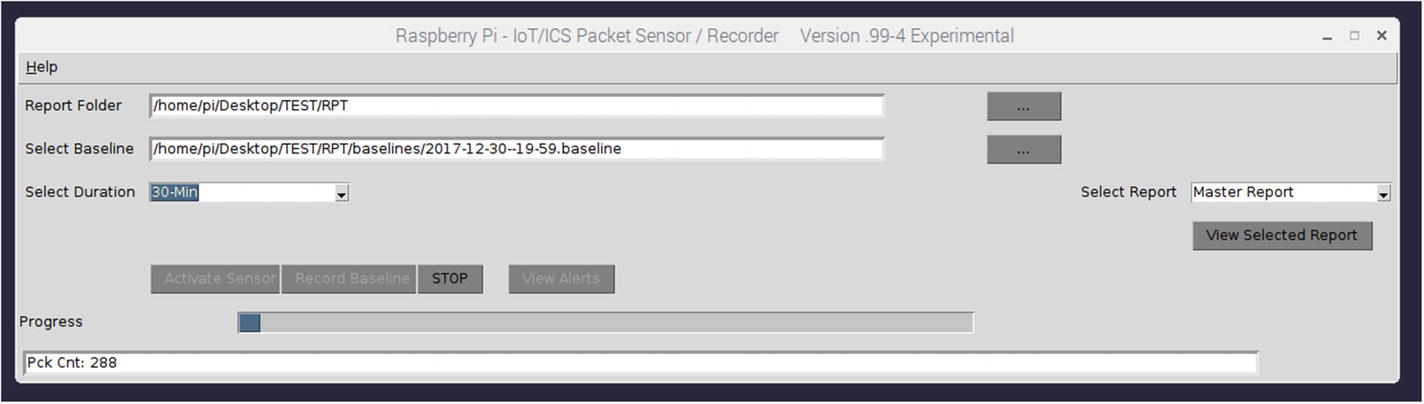
Activating the sensor
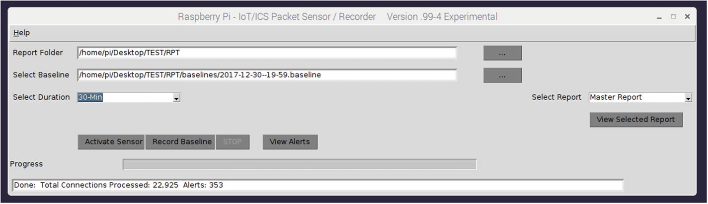
Sensor completed
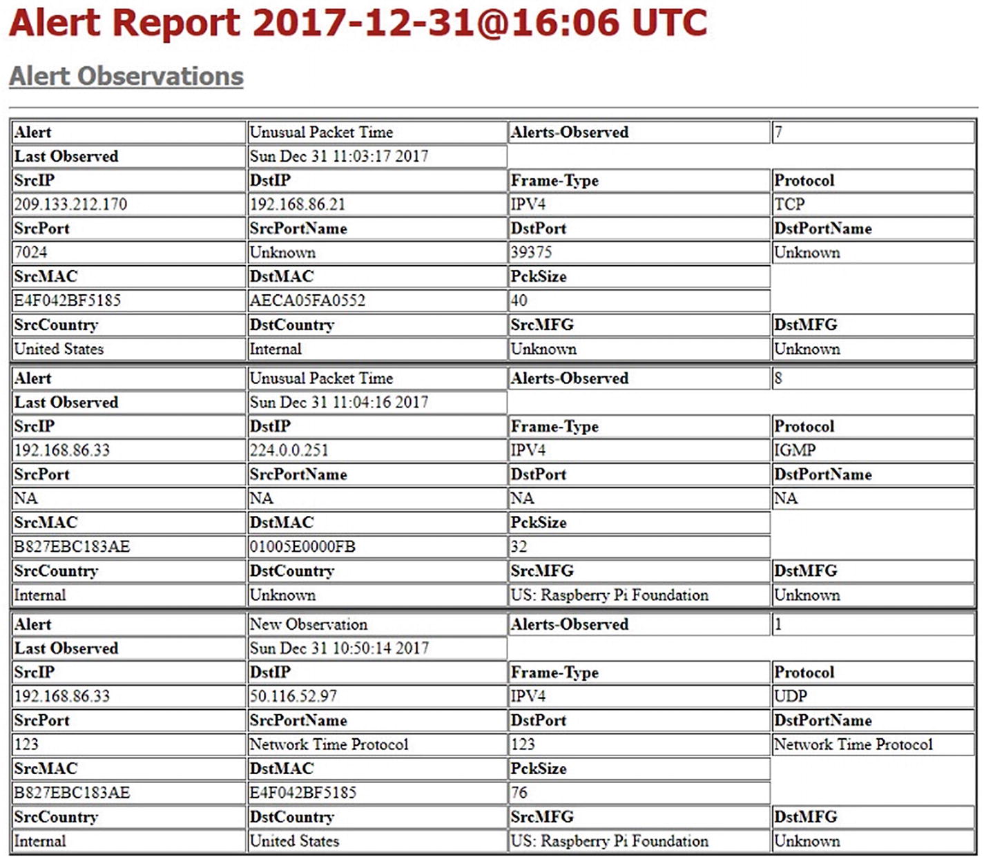
Alert report sample
Summary
Overview of the sensor connection to an active network.
Recording a baseline.
Generating and examining reports created during the process of recording a baseline.
Selection of a recorded baseline once created for use during the sensor phase.
Activation of the sensor based on a specific recorded baseline.
Examination of alerts generated by the sensor.
In Chapter 6, we will take a detailed look at the recording of the baseline process, and the method of reduction that is accomplished using a Python dictionary. In addition, we will examine the details of the sensor decision-making process and baseline comparison.