
Data science and scientific computing are human-centered, collaborative endeavors that gather teams of experts covering multiple domains. You will rarely perform any serious data analysis task alone. Therefore, efficient intra-team communication that ensures proper information exchange within a team is required. There is also a need to convey all details of an analysis to relevant external parties. Your team is part of a larger scientific community, so others must be able to easily validate and verify your team’s findings. Reproducibility of an analysis is as important as the result itself. Achieving this requirement—to effectively deliver data, programs, and associated narrative as an interactive bundle—is not a trivial task. You cannot assume that everybody who wants to peek into your analysis is an experienced software engineer. On the other hand, all stakeholders aspire to make decisions based on available data. Fortunately, there is a powerful open-source solution for reconciling differences in individuals’ skill sets. This chapter introduces the project Jupyter (see https://jupyter.org ), the most popular ecosystem for documenting and sharing data science work.
Notebook document format: A JSON document format for storing all types of content (code, images, videos, HTML, Markdown, LaTeX equations, etc.). The format has the extension .ipynb. See https://github.com/jupyter/nbformat .
Messaging protocol: A network messaging protocol based on JSON payloads for web clients (such as Jupyter Notebook) to talk to programming language kernels. A kernel is an engine for executing live code inside notebooks. The protocol specifies ZeroMQ or WebSockets as a transport mechanism. See https://github.com/jupyter/jupyter_client .
Notebook server: A server that exposes WebSocket and HTTP Resource APIs for clients to remotely access a file system, terminal, and kernels. See https://github.com/jupyter/jupyter_server .
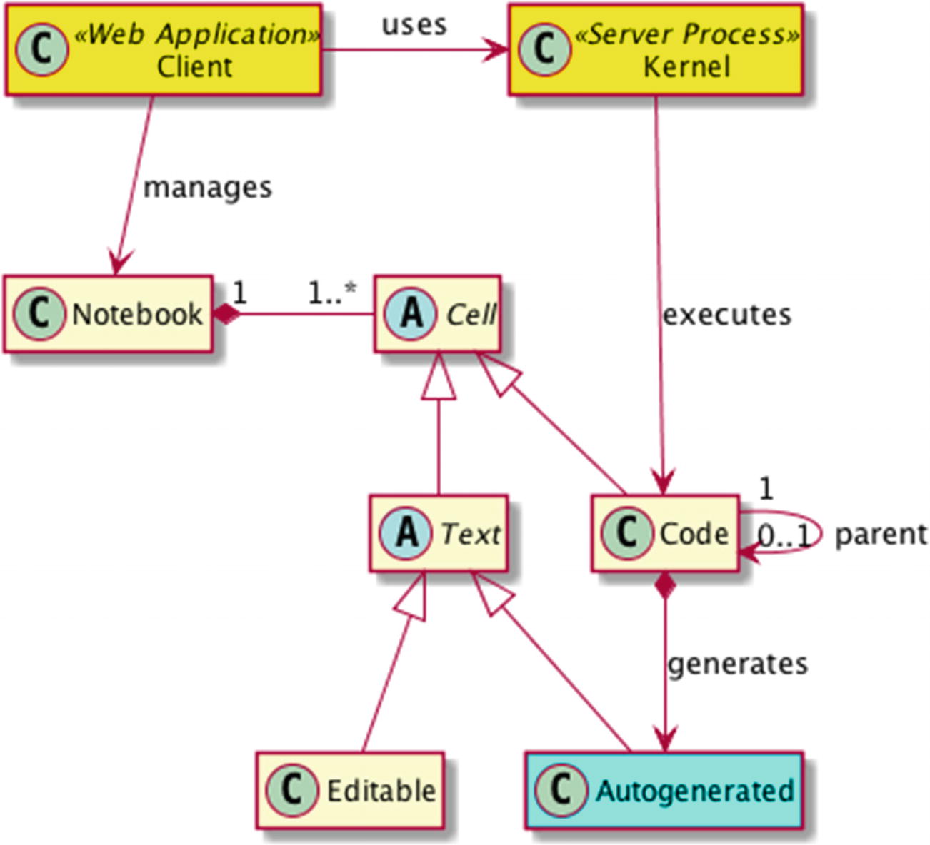
The major components of the Jupyter architecture as well as the structural decomposition of a notebook. Each notebook is associated with its dedicated kernel at any given point in time.
Jupyter Notebook: The first client/server stack of the architecture, which is still widely used at the time of writing.
JupyterLab: The next-generation web client application for working with notebooks.2 We will implement it in this chapter. A notebook created with JupyterLab is fully compatible with Jupyter Notebook and vice versa.
JupyterHub: A cloud-based hosting solution for working with notebooks. It is especially important for enabling large organizations to scale their Jupyter deployments in a secure manner. Superb examples are UC Berkeley’s “Foundations of Data Science” and UC San Diego’s “Data Science MicroMasters” MOOC programs on the edX platform.
IPython: The Python kernel that enables users to use all extensions of the IPython console in their notebooks. This includes invoking shell commands prefixed with !. There are also magic commands for performing shell operations (such as %cd for changing the current working directory). You may want to explore the many IPython-related tutorials at https://github.com/ipython/ipython-in-depth .
Jupyter widgets and notebook extensions: All sorts of web widgets to bolster interactivity of notebooks as well as extensions to boost your notebooks. We will demonstrate some of them in this chapter. For a good collection of extensions, visit https://github.com/ipython-contrib/jupyter_contrib_nbextensions .
nbconvert: Converts a notebook into another rich content format (e.g., Markdown, HTML, LaTeX, PDF, etc.). See https://github.com/jupyter/nbconvert .
nbviewer: A system for sharing notebooks. You can provide a URL that points to your notebook, and the tool will produce a static HTML web page with a stable link. You may later share this link with your peers. See https://github.com/jupyter/nbviewer .
JupyterLab in Action
The top menu bar includes commands to create, load, save, and close notebooks, create, delete, and alter cells, run cells, control the kernel, change views, read and update settings, and reach various help documents.
The left pane has tabs for browsing the file systems, supervising the running notebooks, accessing all available commands, setting the properties of cells, and seeing what tabs are open in the right pane. The file browser’s tab is selected by default and allows you to work with directories and files on the notebook server (this is the logical root). If you run everything locally (your server’s URL will be something like http://localhost:88xx/lab), then this will be your home folder.
The right pane has tabs for active components. The Launcher (present by default) contains buttons to fire up a new notebook, open an IPython console, open a Terminal window, and open a text editor. Newly opened components will be tiled in this area.
Experimenting with Code Execution
In the spirit of data science, let’s first do some experiments with code execution. The goal is to get a sense of what happens when things go wrong, since being able to quickly debug issues increases productivity. Inside the file browser, click the toolbar button to create a new folder (the standard folder button with a plus sign on it). Right-click the newly created folder and rename it to hanoi. Double-click it to switch into that directory. Now, click the button in the Launcher in the right pane to open a notebook. Right-click inside the file browser on the new notebook file and rename it to Solver1.ipubn. If you have done everything properly, then you should see something similar to the screen shown in Figure 4-2.
Tip
If you have made an error, don’t worry. You can always delete and move items by using the context menu and/or drag-and-drop actions. Furthermore, everything you do from JupyterLab is visible in your favorite file handler, so you can fix things from there, too. I advise you to always create a designated directory for your project. This avoids clutter and aids in organizing your artifacts. You will need to reference many other items (e.g., images, videos, data files, etc.) from your notebook. Keeping these together is the best way to proceed.
Hanoi Tower Solver with a Syntax Error
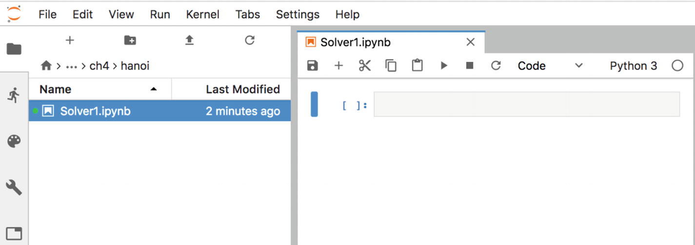
The newly created notebook opened in the right pane
The first cell is empty, and you may start typing in your code. Notice that its type is Code, which is shown in the drop-down box. Every cell is demarcated with a rectangle, and the currently active one has a thick bar on its left side. The field surrounded by square brackets is the placeholder for the cell’s number. A cell receives a new identifier each time after being run. There are two types of numerated cells (see Figure 4-1): editable code cell (its content is preserved inside the In collection) and auto-generated cell (its content is preserved inside the Out collection). For example, you can refer to a cell’s output by typing Out[X], where X is the cell’s identifier. An immediate parent’s output can be referenced via _, such as _X for a parent of X. Finally, the history is searchable and you may press the Up and Down keys to find the desired statement.
The error message in the output from Listing 4-1 is correct about encountering a syntax error. Nonetheless, the explanation is not that helpful, and is even misleading. Observe the bold characters in the error report. The caret symbol is Python’s guess about the location of the error, while the real error is earlier. It is caused by an imbalanced string marker. You may use either " or ' to delineate a string in Python, but do not mix them for the same string.
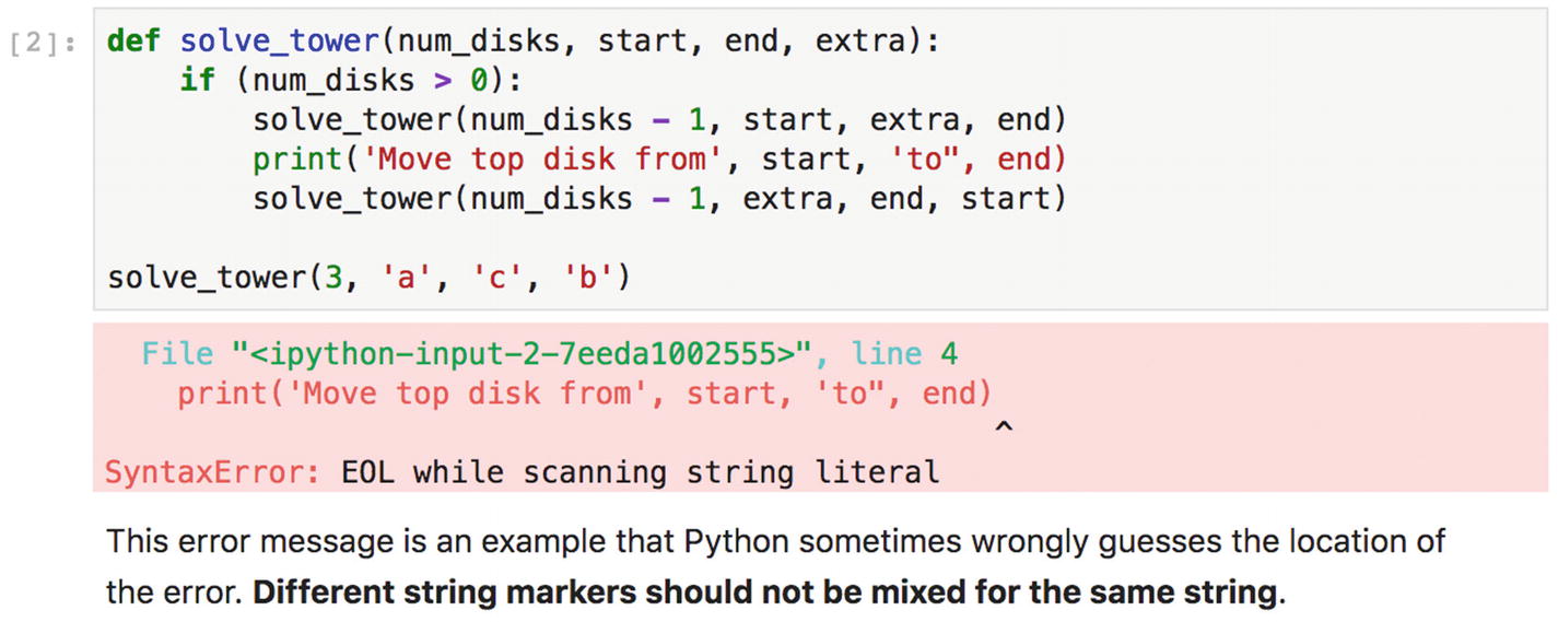
Your first completed notebook showing an edge case of Python’s error reporting. Notice that anyone can see all the details without running the code.
Now save your notebook by clicking the disk icon button in the toolbar. Afterward, close the notebook’s window and shut it down (choose the tab with a symbol of a runner in the left pane and select SHUTDOWN next to your notebook). Simply closing the UI page does not terminate the dedicated background process, so your notebook will keep running.
Hanoi Tower Solver with Infinite Recursion
After all, the critical programming concerns of software engineering and artificial intelligence tend to coalesce as the systems under investigation become larger.
—Alan J. Perlis, Foreword to Structure and Interpretation of Computer Programs, Second Edition (MIT Press, 1996)
Correct Hanoi Tower Solver with Embedded Documentation and Type Annotations
Finally, such documentation can be easily retrieved by executing solve_tower? (if you include two question marks, then you can dump the source code, too).
Managing the Kernel
Interrupt Kernel: Interrupts your current kernel. This is useful when all system components are healthy except your currently running code (we have already seen this command in action).
Restart Kernel...: Restarts the engine itself. You should try this if you notice sluggish performance of your notebook.
Restart Kernel and Clear...: Restarts the server and clears all autogenerated output.
Restart Kernel and Run All...: Restarts the server and runs all code cells from the beginning of your notebook.
Shutdown Kernel: Shuts down your current kernel.
Shutdown All Kernels...: Shuts down all active kernels. This applies when your notebook contains code written in different supported programming languages.
Change Kernel...: Changes your current kernel. You can choose a new kernel from the drop-down list. One of them is the dummy kernel called No Kernel (with this, all attempts to execute a code cell will simply wipe out its previously generated output). You can also choose a kernel from your previous session.
Note
Whenever you restart the kernel, you must execute your code cells again in proper order. Forgetting this is the most probable cause for an error like NameError: name <XXX> is not defined.
Connecting to a Notebook’s Kernel
If you would like to experiment with various variants of your code without disturbing the main flow of your notebook, you can attach another front end (like a terminal console or Qt Console application) to the currently running kernel. To find out the necessary connection information, run inside a code cell the %connect_info magic command.3 The output will also give you some hints about how to make a connection. The nice thing about this is that you will have access to all artifacts from your notebook.
Caution
Make sure to always treat your notebook as a source of truth. You can easily introduce a new variable via your console, and it will appear as defined in your notebook, too. Don’t forget to put that definition back where it belongs, if you deem it to be useful.
Descending Ball Project
We will now develop a small but complete project to showcase other powerful features of JupyterLab (many of them are delivered by IPython, as this is our kernel). The idea is to make the example straightforward so that you can focus only on JupyterLab. Start by creating a new folder for this project (name it ball_descend). Inside it create a new notebook, Simulation.ipubn. Revisit the “Experimenting with Code Execution” section for instructions on how to accomplish these steps.
Problem Specification
You should utilize the rich formatting options provided by the Markdown format. Here, we define headers to create some structure in our document. We will talk more about structuring in the next section. Once you execute this cell, it will be rendered as HTML.
It turns out that the title contains a small typo (the issue is more apparent in the rendered HTML); it says Bal's instead of Ball's. Double-click the text cell, correct the problem, and rerun the cell.
You also could have entered the preceding text using multiple consecutive cells. It is possible to split, merge, and move around cells by using the commands from the Edit menu or by using drag-and-drop techniques. The result of running a text cell is its formatted output. Text cells may be run in any order. This is not the case with code cells. They usually have dependencies on each other. Forgetting to run a cell on which your code depends may cause all sorts of errors. Obviously, reducing coupling between code cells is vital. A graph of dependencies between code cells may reveal a lot about complexity. This is one reason why you should minimize dependencies on global variables, as these intertwine your cells.
Model Definition
Global Imports for the Notebook with a Comment for the User to Just Run It
Your notebook should be carefully organized with well-defined sections. Usually, bootstrapping code (such as shown in Listing 4-4) should be kept inside a single code cell at the very beginning of your notebook. Such code is not inherently related to your work, and thus should not be spread out all over your notebook. Moreover, most other code cells depend on this cell to be executed first. If you alter this section, then you should rerun all dependent cells. A handy way to accomplish this is to invoke Run ➤ Run Selected Cell and All Below.
Definition of Our Data Model
A cell may hold multiple lines and expressions. Such a composite cell executes by sequentially running the contained expressions (in the order in which they appear). Here, we have an assignment and a value expression. The latter is useful to see the effect of the assignment (assignments are silently executed). Remember that a cell’s output value is always the value of its last expression (an assignment has no value). If you want to dump multiple messages, you can use Python’s print statement (these messages will not count as output values) with or without a last expression. Typically, an output value will be nicely rendered into HTML, which isn’t the case with printed output. This will be evident when we output as a value a Pandas data frame in Chapter 5.
It is also possible to prevent outputting the last expression’s value by ending it with a semicolon. This can be handy in situations where you just want to see the effects of calling some function (most often related to visualization).
When your cursor is inside a multiline cell, you can use the Up and Down arrows on your keyboard to move among those lines. To use your keys to move between cells, you must first escape the block by pressing the Esc key. It is also possible to select a whole cell by clicking inside an area between the left edge of a cell and the matching thick vertical bar. Clicking the vertical bar will shrink or expand the cell (a squashed cell is represented with three dots).
Tip
It is possible to control the rendering mechanism for output values by toggling pretty printing on and off. This can be achieved by running the %pprint magic command. For a list of available magic commands, execute %lsmagic.
Note
Never put inside the same cell a slow expression that always results in the same value (like reading from a file) and an idempotent parameterized expression (like showing the first couple of elements of a data frame). The last expression cannot be executed independently (i.e., without continuously reloading the input file).
The matrix function is just one of many from the NumPy package. JupyterLab’s context-sensitive typing facility can help you a lot. Just press the Tab key after np., and you will get a list of available functions. Further typing (for example, pressing the M key) will narrow down the list of choices (for example, to names starting with m). Moreover, issuing np.matrix? in a code cell provides you with help information about this function (you must execute the cell to see the message). Executing np? gives you help about the whole framework.
Path Finder’s Implementation
Definition of the wall Function to Detect Borders
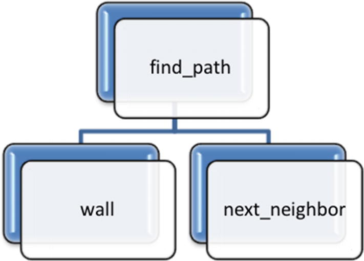
Top-down decomposition of our problem; we will implement the functions via the bottom-up method
Implementation of the Other Two Functions As Shown in Figure 4-4
The find_path function is a very simple recursive function. The exit condition is the guaranteed local minima (unless you model a terrain from Escher’s world), since we monotonically descend toward the lowest neighbor.
After executing all cells, we should receive a test result with no errors. Notice that all functions are self-contained and independent from the environment. This is very important from the viewpoint of maintenance and evolution. Interestingly, all functions would execute perfectly even if you were to remove the terrain argument from their signature. Nonetheless, dependence on global variables is an equally bad practice in notebooks as it is anywhere else. It is easy to introduce unwanted side-effects and pesky bugs. Nobody has time, nor incentive, to debug your document to validate your results!
Interaction with the Simulator
After you execute this cell, you will be presented with two named sliders to set the ball’s initial position (X represents the row and Y the column). Each time you move the slider, the system will output a new path. There is no chance to provide an invalid starting position, as the sliders are configured to match the terrain’s shape. The notebook included in this book’s source code bundle also contains some narrative for presenting the result inside a separate section.
Test Automation
Refactoring the Simulator’s Notebook
- 1.
Move out the wall, next_neighbor, and find_path functions into a separate package called pathfinder.
- 2.
Move the doctest call into our new package.
- 3.
Import the new package into our notebook (we need to access the find_path function).
- 4.
Add more explanation about what we are doing, together with a nicely formatted formula.
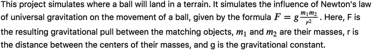
The LaTex content inside ordinary text is beautifully rendered into HTML
Document Structure
In our previous project, we have already tackled the topic of content structuring, although in a really lightweight fashion. We will devote more attention to it here. Whatever technology you plan to use for your documentation task, you need to have a firm idea of how to structure your document. A structure brings order and consistency to your report. There are no hard rules about this structure, but there are many heuristics (a.k.a. best practices). The document should be divided into well-defined sections arranged into some logical order. Each section should have a clear scope and volume; for example, it makes no sense to devote more space to the introduction than to the key findings in your analysis. Remember that a notebook is also a kind of document and it must be properly laid out. Sure, the data science process already advises how and in what order to perform the major steps (see Chapter 1), and this aspect should be reflected in your notebook. Nonetheless, there are other structuring rules that should be superimposed on top of the data science life cycle model.
Abstract: This section should be a brief summary of your work. It must illuminate what you have done, in what way, and enumerate key results.
Motivation: This section should explain why your work is important and how it may impact the target audience.
Dataset: This section should describe the dataset and its source(s). You should give unambiguous instructions that explain how to retrieve the dataset for reproducibility purposes.
Data Science Life Cycle Phases: The next couple of sections should follow the data science life cycle model (date preprocessing, research questions, methods, data analysis, reporting, etc.) and succinctly explain each phase. These details are frequently present in data analysis notebooks.
Drawbacks: This section should honestly mention all limitations of your methodology. Not knowing about constraints is very dangerous in decision making.
Conclusion: This section should elaborate about major achievements.
Future Work: This section should give some hints about what you are planning to do in the future. Other scientists are dealing with similar issues, and this opens up an opportunity for collaboration.
References: This section should list all pertinent references that you have used during your research. Don’t bloat this section as an attempt to make your work more “convincing.”
The users of your work may be segregated into three major categories: the general public, decision makers, and technically savvy users. The general public is only interested in what you are trying to solve. Users in this category likely will read only the title and abstract. The decision makers are business people and are likely to read the major findings as well as the drawbacks and conclusion. They mostly seek well-formulated actionable insights. The technical people (including CTOs, data scientists, etc.) would also like to reproduce your findings and extend your research. Therefore, they will look into all aspects of your report, including implementation details. If you fail to recognize and/or address the needs of these various classes of users, then you will reduce the potential to spread your results as broadly as possible.
Wikipedia Edits Project
As an illustration of the template outlined in the previous section, I will fill out some of the sections based upon my analysis of Wikipedia edits. The complete Jupyter notebook is publicly available at Kaggle (see https://www.kaggle.com/evarga/analysis-of-wikipedia-edits ). It does contain details about major data science life cycle phases. The goal of this project is to spark discussion, as there are many points open for debate. The following sections from the template should be enough for you to grasp the essence of this analysis (without even opening the previously mentioned notebook). Don’t worry if the Kaggle notebook seems complicated at this moment.
Abstract
This study uses the Wikipedia Edits dataset from Kaggle. It tries to inform the user whether Wikipedia’s content is stable and accountable. The report also identifies which topics are most frequently edited, based on words in edited titles. The work relies on various visualizations (like scatter plot, stacked bar graphs, and word cloud) to drive conclusions. It also leverages NLTK to process the titles. We may conclude that Wikipedia is good enough for informal usage with proper accountability, and themes like movies, sports, and music are most frequently updated.
Motivation
Wikipedia often is the first web site that people visit when they are looking for information. Obviously, high quality (accuracy, reliability, timeliness, etc.) of its content is imperative for a broad community. This work tries to peek under the hood of Wikipedia by analyzing the edits made by users. Wikipedia can be edited by anyone (including bots), and this may raise concerns about its trustworthiness. Therefore, by getting more insight about the changes, we can judge whether Wikipedia can be treated as a reliable source of information. As a side note, scientific papers cannot rely on it. There are also some book publishers who forbid referencing Wikipedia. All in all, this report tries to shed light on whether Wikipedia is good enough for informal usage.
Drawbacks
The data reflects an activity of users over a very short period of time. Such a small dataset cannot provide a complete story. Moreover, due to time zone differences, it cannot represent all parts of the world.
There is no description on Kaggle about the data acquisition process for the downloaded dataset. Consequently, the recorded facts should be taken with a pinch of salt. The edit’s size field is especially troublesome.
The data has inherent limitations, too. I had no access to the user profiles, so I assumed all users are equally qualified to make edits. If I would have had this access, then I could have weighted the impact of their modifications.
Conclusion
Wikipedia is good enough for informal usage. The changes are mostly about fixing smaller issues. Larger changes in size are related mostly to addition of new content and are performed by humans. These updates are treated as major.
Larger edits are done by registered users, while smaller fixes are performed also by anonymous persons.
Specialized content (scientific, technical/technology related, etc.) doesn’t change as frequently as topics about movies, sport, music, etc.
Exercise 4-1. External Load of Data
Manually entering huge amounts of data doesn’t scale. In our case study, the terrain’s configuration fits into a 5×4 matrix. Using this approach to insert elevations for a 200×300 terrain would be impossible. A better tactic is to store data externally and load it on demand. Modify the terrain’s initialization code cell to read data from a text file. Luckily, you don’t need to wrestle with this improvement too much. NumPy’s Matrix class already supports data as a string. Here is an excerpt from its documentation: “If data is a string, it is interpreted as a matrix with commas or spaces separating columns, and semicolons separating rows.”
You would want to first produce a text file with the same content as we have used here. In this way, you can easily test whether everything else works as expected. You should upload the configuration file into the same folder where your notebook is situated (to be able to use only the file name as a reference). To upload stuff, click the Upload Files toolbar button in JupyterLab’s file browser. Refer to Chapter 2 for guidance on how to open/read a text file in Python.
Exercise 4-2. Fixing Specification Ambiguities
Thanks to the accessibility of your JupyterLab notebook and the repeatability of your data analysis, one astute data scientist has noticed a flaw in your solution. He reported this problem with a complete executable example (he shared with you a modified notebook file). Hence, you can exactly figure out what he would like you to fix. For a starting position (0, 1) it is not clear in advance whether the ball should land in (0, 0) or (1, 0), since they are both at a locally lowest altitude (in this case -2). It is also not clear where the ball should go if it happens to land on a plateau (an area of the terrain at the same elevation). In the current solution, it will stop on one of the spots, depending on the search order of neighbors. Surely, this doesn’t quite satisfy the rule of stopping at the local minima.
The questions are thus: Should you consider inertia? How do you document what point will be the final point? Think about these questions and expand the text and/or modify the path-finding algorithm.
Exercise 4-3. Extending the Project
Another data scientist has requested an extension of the problem. She would like to ascribe elasticity to the ball. If it drops more than X units, then it could bounce up Y units. Change the path-finding algorithm to take this flexibility into account. Assume that the ball will still select the lowest neighbor, although the set of candidates will increase. Will the recursion in find_path always terminate? What conditions dictate such guaranteed termination? Test your solution thoroughly.
Exercise 4-4. Notebook Presentation
In the “Document Structure” section, you can find the proposed document template. Creating a separate artifact, external to your main notebook, isn’t a good choice, since it will eventually drift away from it (like passive design documents in software development).
A new browser window will open, presenting one after another cells marked as Slide. Look up the meaning of other slide types: Sub-slide, Fragment, and Notes. Consult JupyterLab’s documentation for more information about presentation mode. For a really professional presentation, you should use Reveal.js (see https://revealjs.com ).
Summary
Freeform text is bundled together with executable code; this eliminates the need to maintain separate documents, which usually get out of sync with code.
The output of code execution may be saved in the document and become an integral part of it.
The setup of an executable environment (to bring in dependencies for running your code) may be done inside the document. This solves many deployment problems and eliminates a steep learning curve for those who would like to see your findings in action.
You have witnessed the power behind computational notebooks and how the Jupyter toolset accomplishes most requirements regarding documentation. By supporting disparate programming languages, JupyterLab fosters polyglot programming, which is important in the realm of data science. In the same way as multiple data sources are invaluable, many differently optimized development/executable environments are indispensable in crafting good solutions.
JupyterLab has many more useful features not demonstrated here. For example, it has a web-first code editor that eliminates the need for a full-blown integrated development environment (such as Spyder) for smaller edits. You can edit Python code online far away from your machine. JupyterLab also allows you to handle data without writing Python code. If you open a Leaflet GeoJSON file (see https://leafletjs.com ), then it will be immediately visualized and ready for interaction. A classical approach entails running a Python code cell.
All in all, this chapter has provided the foundation upon which further chapters will build. We will continually showcase new elements of JupyterLab, as this will be our default executable environment.
References
- 1.
Brian Granger, “Project Jupyter: From Computational Notebooks to Large Scale Data Science with Sensitive Data,” ACM Learning Seminar, September 2018.
- 2.
Matt Cone, The Markdown Guide, https://www.markdownguide.org .
- 3.
Jake VanderPlas, Python Data Science Handbook: Essential Tools for Working with Data, O’Reilly Media, Inc., 2016.
- 4.
Mike Grouchy, “Be Pythonic: __init__.py,” https://mikegrouchy.com/blog/be-pythonic-__init__py , May 17, 2012.