© Ervin Varga 2019
E. Varga Practical Data Science with Python 3https://doi.org/10.1007/978-1-4842-4859-1_5

5. Data Processing

Ervin Varga1 
(1)
Kikinda, Serbia
 

Data analysis is the central phase of a data science process. It is similar to the construction phase in software development, where actual code is produced. The focus is on being able to handle large volumes of data to synthesize an actionable insight and knowledge. Data processing is the major phase where math and software engineering skills interplay to cope with all sorts of scalability issues (size, velocity, complexity, etc.). It isn’t enough to simply pile up various technologies in the hope that all will auto-magically align and deliver the intended outcome. Knowing the basic paradigms and mechanisms is indispensable. This is the main topic of this chapter: to introduce and exemplify pertinent concepts related to scalable data processing. Once you properly understand these concepts, then you will be in a much better position to comprehend why a particular choice of technologies would be the best way to go.

Augmented Descending Ball Project

We will expand on the example from the previous chapter. As a reminder, here is the original problem specification in Markdown format (the bold section will be altered):
# Simulation of a Ball's Descent in a Terrain
This project simulates where a ball will land in a terrain.
## Input
The terrain's configuration is given as a matrix of integers representing elevation at each spot. For simplicity, assume that the terrain is surrounded by a rectangular wall that prevents the ball from escaping. The inner dimensions of the terrain are NxM, where N and M are integers between 3 and 1000.
The ball's initial position is given as a pair of integers (a, b).
## Output
The result is a list of coordinates denoting the ball's path in a terrain. The first element of the list is the starting position, and the last one is the ending position. It could happen that they are the same, if the terrain is flat or the ball is dropped at the lowest point (the local minima).
## Rules
The ball moves according to the next two simple rules:
- The ball rolls from the current position into the lowest neighboring one.
- If the ball is surrounded by higher points, then it stops.

Version 1.1

Data science is all about combining different data sources in a meaningful way (dictated by business drivers). To make our product more useful for a broader community, we will extend the initial system to accept as input some real terrain’s elevation data encoded in an image; open the Terrain_Simulation_v1.1.ipubn notebook in the augmented_ball_descend source folder of this chapter. The rest of the specification should remain valid. Figure 5-1 presents one publicly available satellite image dataset from the WIFIRE Lab (visit https://wifire.ucsd.edu ), which is also used in UC San Diego’s MOOC Python for Data Science on edX. The WIFIRE system gets these images from an external source, NASA’s Global Imagery Browse Services (GIBS) (see https://earthdata.nasa.gov , where GIBS is accessible from the DATA tab).
../images/473947_1_En_5_Chapter/473947_1_En_5_Fig1_HTML.jpg
Figure 5-1

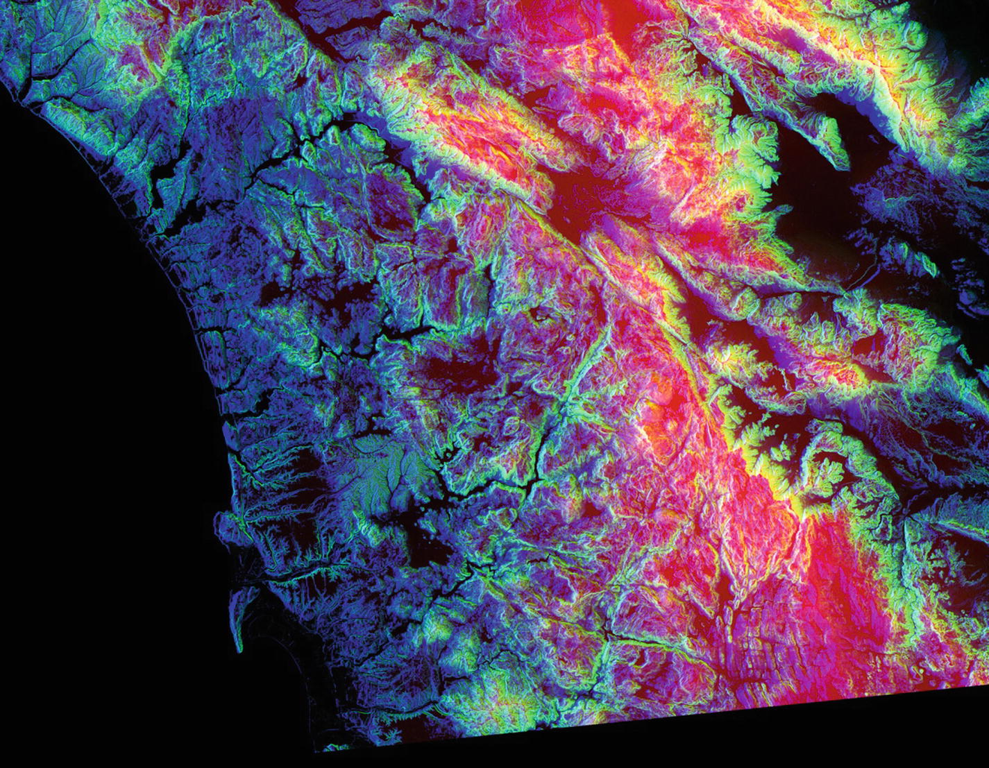
The satellite image of a coastline with encoded terrain data; each pixel’s red-green-blue components represent altitude, slope, and aspect, respectively. Higher color component values denote higher altitude, slope, and aspect.

The following is the new description of what we expect as input (notice how coloring is done in Markdown):
The terrain's configuration is given as a matrix of integers representing elevation at each spot. This matrix is computed from a satellite image of a terrain that encodes altitude inside a pixel's <span style="color:red">∗RED∗</span> color component. For simplicity, assume that the terrain is surrounded by a wall, that prevents the ball to escape. The inner dimensions of the terrain are NxM, where N and M are integers.
The ball's initial position is given as a pair of integers (a, b).
The following snippet of code reads the image and dumps some statistics (the following couple of imports have been spread out over the notebook to highlight the changes):
import imageio
terrain = imageio.imread('terrain_data/coastline.jpg')
print("The terrain's dimensions are %s with minimum %i, maximum %i, and mean %.2f for points."%
      (terrain.shape, terrain.min(), terrain.max(), terrain.mean()))
Running this cell produces the following output:
The terrain's dimensions are (3725, 4797, 3) with minimum 0, maximum 255, and mean 75.83 ➥
for points.
So, the size of the input is increased from 5×4 to 3725×4797×3. The following lines display the image as depicted in Figure 5-1:
%matplotlib inline
import matplotlib.pyplot as plt
plt.figure(figsize=(13, 15))
plt.imshow(terrain);

Boundaries and Movement

The path finder module from Chapter 4 cannot be reused directly. Currently, altitude is encoded as an integer from range [0, 255] and we may expect many points to share altitude. Consequently, we must also consult the slope to decide about the lowest neighbor. Therefore, there is a need to more precisely describe the lowest neighbor concept as follows:
  • An adjacent point with the lowest altitude is the lowest neighbor.

  • An adjacent point with the same altitude (if the others are at higher altitude) is the lowest neighbor, if the current point’s slope is greater than zero.

  • If there are multiple adjacent points satisfying the previous condition, then one of them is chosen in clockwise direction starting at south-west.

We obviously don’t need the blue color component (aspect). The next line of code sets this layer to zero:
terrain[:, :, 2] = 0

Path Finding Engine

The original version of the path finding engine was implemented as a set of routines. To enhance maintainability, we will re-engineer the code to use object-oriented constructs. Listing 5-1 shows the backbone structure. This is the content of the base_patfinder.py file (it passes the Spyder’s static code analyzer with maximum score 10/10). Notice how the embedded documentation for abstract methods doesn’t mention anything about specific implementation details. These should be left to child classes.
"""The base class for implementing various path finders."""
import abc
from typing import List, Tuple, Set
import numpy as np
class BasePathFinder(metaclass=abc.ABCMeta):
    """
    Finds the path of a ball that descends in a terrain from some starting
    position.
    Args:
    terrain: the terrain's configuration comprised from (altitude, slope)
    integer pairs.
    """
    def __init__(self, terrain: np.ndarray):
        self._terrain = terrain
    @property
    def terrain(self):
        """Gets the current terrain data."""
        return self._terrain
    def wall(self, position: Tuple[int, int]) -> bool:
        """
        Checks whether the provided position is hitting the wall .
        Args:
        position: the pair of integers representing the ball's potential position.
        Output:
        True if the position is hitting the wall, or False otherwise.
        Examples:
        >>> BasePathFinder.__abstractmethods__ = set()
        >>> path_finder = BasePathFinder(np.array([[(-2, 0), (3, 0), (2, 0), (1, 0)]]))
        >>> path_finder.wall((0, 1))
        False
        >>> BasePathFinder.__abstractmethods__ = set()
        >>> path_finder = BasePathFinder(np.array([[(-2, 0), (3, 0), (2, 0), (1, 0)]]))
        >>> path_finder.wall((-1, 0))
        True
        """
        curr_x, curr_y = position
        length, width = self.terrain.shape[:2]
        return (curr_x < 0) or (curr_y < 0) or (curr_x >= length) or (curr_y >= width)
    @abc.abstractmethod
    def next_neighbor(self, position: Tuple[int, int],
                      visited: Set[Tuple[int, int]]) -> Tuple[int, int]:
        """
        Returns the position of the lowest neighbor or the current position.
        Args:
        position: the pair of integers representing the ball's current position.
        visited: the set of visited points.
        Output:
        The position (pair of coordinates) of the lowest neighbor .
        """
    @abc.abstractmethod
    def find_path(self, position: Tuple[int, int],
                  visited: Set[Tuple[int, int]]) -> List[Tuple[int, int]]:
        """
        Finds the path that the ball would follow while descending in the terrain.
        Args:
        position: the pair of integers representing the ball's current position.
        visited: the set of visited points (may be preset to avoid certain points).
        Output:
        The list of coordinates of the path.
        """
if __name__ == "__main__":
    import doctest
    doctest.testmod()
Listing 5-1

Restructured Path Finding Module, Which Uses Object-Oriented Programming

Listing 5-2 shows our first attempt to implement the logic.
"""Simple recursive path finder implementation ."""
from typing import List, Tuple, Set
from pathfinder.base_pathfinder import BasePathFinder
class SimplePathFinder(BasePathFinder):
    """Concrete path finder that uses recursion and is sequential."""
    def next_neighbor(self, position: Tuple[int, int],
                      visited: Set[Tuple[int, int]]) -> Tuple[int, int]:
        """
        Uses a simple clockwise search of neighbors starting at south-west.
        Example:
        >>> path_finder = SimplePathFinder(np.array([[(-2, 0), (3, 0), (2, 0), (1, 0)]]))
        >>> path_finder.next_neighbor((0, 1), set((0, 1)))
        (0, 0)
        """
        curr_x, curr_y = position
        current_slope = self.terrain[position][1]
        min_altitude = self.terrain[position][0]
        min_position = position
        for delta_x in range(-1, 2):
            for delta_y in range(-1, 2):
                new_position = (curr_x + delta_x, curr_y + delta_y)
                if not self.wall(new_position) and not new_position in visited:
                    new_altitude = self.terrain[new_position][0]
                    if new_altitude < min_altitude or (new_altitude == min_altitude and
                                            current_slope > 0):
                        min_altitude = new_altitude
                        min_position = new_position
        return min_position
    def find_path(self, position: Tuple[int, int],
                  visited: Set[Tuple[int, int]] = None) -> List[Tuple[int, int]]:
        """
        Recursively finds the path.
        Example:
        >>> path_finder = SimplePathFinder(np.array([[(-1, 2), (-2, 1), (-2, 2), (1, 0)]]))
        >>> path_finder.find_path((0, 2))
        [(0, 2), (0, 1)]
        """
        if visited is None:
            visited = set()
        visited.add(position)
        next_position = self.next_neighbor(position, visited)
        if position == next_position:
            return [position]
        return [position] + self.find_path(next_position, visited)
if __name__ == "__main__":
    import doctest
    doctest.testmod()
Listing 5-2

The Simple Path Finder Class That Uses Recursion to Traverse the Terrain

Even this simple path finder is considerably more complex than our initial variant from Chapter 4. It uses a multidimensional Numpy array instead of a matrix for representing terrain data, has a different logic inside the next_neighbor method , and traces already visited points. Without this last step it could easily trigger an infinite recursion. The next code cell makes a simple test whose output is also shown (marked with >>>):
# Test the simulator with a toy terrain; slope is set to zero, so only altitude matters.
test_terrain = np.array(
    [[(-2, 0), (3, 0),  (2, 0),  (1, 0)],
    [(-2, 0),  (4, 0),  (3, 0),  (0, 0)],
    [(-3, 0),  (3, 0),  (1, 0), (-3, 0)],
    [(-4, 0),  (2, 0), (-1, 0),  (1, 0)],
    [(-5, 0), (-7, 0),  (3, 0),  (0, 0)]])
from pathfinder import SimplePathFinder
path_finder = SimplePathFinder(test_terrain)
path_finder.find_path((1, 1))
>>> [(1, 1), (2, 0), (3, 0), (4, 1)]
All seems to be OK, so we can try it out on our real terrain data. The following snippet of code is reused from the notebook presented in Chapter 4:
path_finder = SimplePathFinder(terrain)
interact(lambda start_x, start_y: path_finder.find_path((start_x, start_y)),
         start_x = widgets.IntSlider(value=1, max=terrain.shape[0]-1, description='Start X'),
         start_y = widgets.IntSlider(value=1, max=terrain.shape[1]-1, description='Start Y'));
By playing around with the sliders, you may watch as paths get calculated. For example, a starting position (2966, 1367) would result in the following path:
[(2966, 1367), (2967, 1368), (2968, 1369), (2969, 1370), (2970, 1371), (2970, 1372), (2971, 1373), (2972, 1374), (2973, 1375), (2974, 1375), (2975, 1375), (2976, 1375), (2977, 1375)]

Retrospective of Version 1.1

Apparently, the input/output subsystems are inapt. Setting a starting position with sliders and getting back a list of coordinates is cumbersome. Sure, it was OK for a toy terrain, but now the situation is different. Where is the point (2966, 1367) located on the map? How do we understand the ball’s movement? Figure 5-2 shows the radar diagram that depicts the level of sophistication achieved across various dimensions in the initial version, and Figure 5-3 shows the level of sophistication achieved in this version.
../images/473947_1_En_5_Chapter/473947_1_En_5_Fig2_HTML.jpg
Figure 5-2

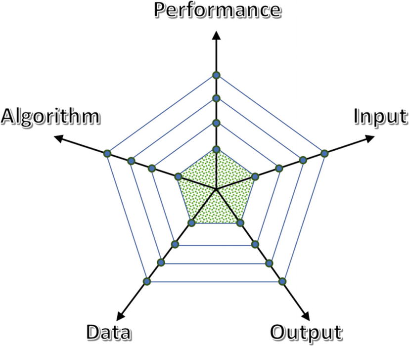
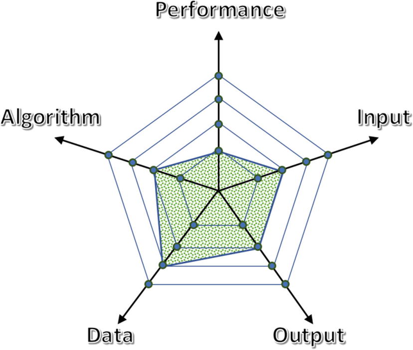
The shaded area represents the overall progress across all dimensions; dimensions may be arbitrarily chosen depending on the context

A system may attain different levels between them, as you will soon see. Our initial version has everything at the basic rank. The data dimension encompasses multiple aspects: volume, velocity, structural complexity, etc. The algorithm dimension represents both mathematical models and computer science algorithms. Input and output denote the capabilities pertaining to data acquisition and presentation of results, respectively. Performance in our case is associated with memory and CPU consumption.
../images/473947_1_En_5_Chapter/473947_1_En_5_Fig3_HTML.jpg
Figure 5-3

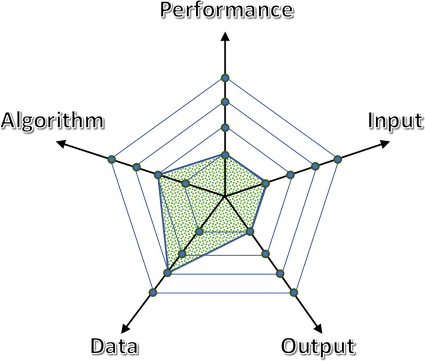
The new version has moved two units on the data axis (bigger size and enhanced structure) and one on the algorithm line

We have already seen that the input and output subsystems are deficient, so these require an improvement.

Retrospectives are regularly used in various Agile methods, too. They create opportunities for discussing lessons learned and potential improvements. Data science endeavors also require retrospectives. As you will see in the upcoming iterations, many times you will discover that there is a need for more exploration, preprocessing, and data-gathering cycles. The whole process is iterative and incremental.

Version 1.2

In this version we will move both the input and output subsystems by one unit; open the Terrain_Simulation_v1.2.ipubn notebook in the augmented_ball_descend source folder of this chapter. The idea is to allow the user to enter the starting position by directly specifying a point on the map. Furthermore, we would like to visualize the output on the map instead of just returning a set of points.

Enhancing the Input Subsystem

Let’s start with Listing 5-3, which shows a small HTML CSS to customize the interactive matplotlib session (matplotlib is discussed in depth in Chapter 6). Try skipping this code cell to see its effect.
%%html
<!-- Removes the default title "Figure 1" and button for an interactive session. -->
<style>
    .output_wrapper .ui-dialog-titlebar {display: None;}
</style>
Listing 5-3

Removes the Default Title and Button for Closing the Interactive Session

Listing 5-4 presents the main section in the notebook to gather input from a user. It uses an auxiliary class that is listed in Listing 5-5 (see also Exercise 5-2 at the end of the chapter). It differentiates between clicking a mouse to select an area of an image and selecting the starting position.
%matplotlib notebook
from ipywidgets import Textarea
from interactionlib import InteractionMonitor
fig = plt.figure()
plt.imshow(terrain)
info_area = Textarea(
    value = ",
    placeholder = 'Select a point on the map by clicking the mouse.',
    description = 'Position:',
    disabled = True
)
display(info_area)
fig.tight_layout(pad = 1.3)
interaction_monitor = InteractionMonitor(fig, info_area)
interaction_monitor.start()
Listing 5-4

Setup of an Interactive Session to Acquire the Starting Position from a User

"""
Monitors whether the user is selecting an area on the image or has chosen the
starting position.
"""
from ipywidgets import Textarea
import matplotlib.pyplot as plt
class InteractionMonitor:
    """
    Detects mouse events to figure out what a user is doing.
    Args:
    fig: the matplotlib figure to monitor.
    info_area: the external informational area whose value needs to be updated.
    auto_stop_interaction: should interaction stop (when True) after selecting
    the starting position or not.
    """
    def __init__(self, fig: plt.Figure, info_area: Textarea,
                 auto_stop_interaction: bool = True):
        self._fig = fig
        self._info_area = info_area
        self._auto_stop_interaction = auto_stop_interaction
        self._cids = None
        self._selecting = False
        self._clicked = False
        self._clicked_position = None
    def _on_click(self, event):
        self._clicked = True
    def _on_release(self, event):
        if not self._selecting:
            self._clicked_position = (int(event.xdata), int(event.ydata))
            self._info_area.value = str(self._clicked_position)
            if self._auto_stop_interaction:
                self.stop()
        self._selecting = False
        self._clicked = False
    def _on_motion(self, event):
        self._selecting = self._clicked
    @property
    def clicked_position(self):
        """Returns the clicked data position on the map."""
        return self._clicked_position
    def start(self):
        """Starts monitoring mouse events on figure."""
        self._cids = [
            self._fig.canvas.mpl_connect('button_press_event', self._on_click),
            self._fig.canvas.mpl_connect('button_release_event', self._on_release),
            self._fig.canvas.mpl_connect('motion_notify_event', self._on_motion)]
    def stop(self):
        """Closes the figure and stops the interaction."""
        plt.close(self._fig)
Listing 5-5

Helper Class to Monitor User Actions

Caution

The previously implemented matplotlib interactive session only works with Jupyter Notebook (at the time of this writing). If you try to run the last code cell inside JupyterLab, you will receive the error Javascript Error: IPython is not defined. This is a fine example of the fact that you must occasionally solve problems completely unrelated to your main objectives.

Figure 5-4 illustrates a session of choosing the starting position. Now it is obvious where the ball will start to descend. All in all, this concludes the input part, although myriad additional enhancements are possible (for example, allowing users to directly enter coordinates, enabling navigation via keyboard, etc.).
../images/473947_1_En_5_Chapter/473947_1_En_5_Fig4_HTML.jpg
Figure 5-4

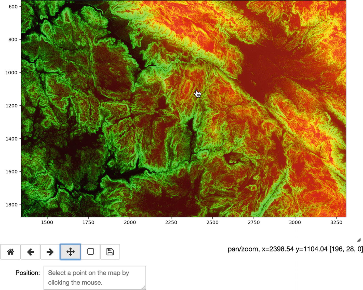
Part of the original image zoomed by a user to easily select a desired point (second button from the right)

You can see that the coordinates on axes reflect this zooming. The actual cursor position is printed on the right side together with data about the current altitude, slope, and aspect (this component is zeroed out so the whole picture is a combination of red and green). The small triangle above the coordinates is for resizing the whole UI. Once a point is selected, the session closes and its coordinates are displayed in the text area on the bottom. Compare this UI with the previous rudimentary slider-based input mechanism.

Enhancing the Output Subsystem

Handling the output will be an easier task. The system just needs to encode the path of a ball using the image’s blue color component (it will be set to 255). This new image may be reused for another run. Accordingly, the notebook will save the final image for later use. Of course, the raw coordinates may still be valuable, so the system should return those, too.

One possible way to achieve the preceding goals is to have a new utility method that will visualize the calculated path on the terrain. The separation-of-concerns principle suggests that we should put this method into a new class, PathUtils. It will require the terrain and path as arguments and will return a new image. Listing 5-6 shows the implementation details of this method, while Listing 5-7 reveals the code cell that manages the workflow. This concludes the work on extending the output subsystem.
"""Contains various path related utility classes and methods."""
from typing import List, Tuple
import numpy as np
class PathUtils:
    """Encompasses static methods to handle paths."""
    @staticmethod
    def encode_path(terrain: np.ndarray, descend_path: List[Tuple[int, int]]) -> np.ndarray:
        """
        Encodes the path into the terrain by setting the points' 3rd (blue) component to 255.
        Args:
        terrain: the terrain's configuration comprised from (altitude, slope, [aspect])
        integer pairs/triples.
        Output:
        New terrain with an extra 3rd dimension to encode the path.
        Example:
        >>> terrain = np.array([[(-1, 2), (-2, 1), (-2, 2), (1, 0)]])
        >>> PathUtils.encode_path(terrain, [(0, 2), (0, 1)])
        array([[[ -1,   2,   0],
                [ -2,   1, 255],
                [ -2,   2, 255],
                [  1,   0,   0]]])
        """
        # Expand terrain with an extra dimension, as needed.
        if terrain.shape[2] == 2:
            new_shape = terrain.shape[:2] + (3,)
            new_terrain = np.zeros(new_shape, terrain.dtype)
            new_terrain[:terrain.shape[0], :terrain.shape[1], :2] = terrain
         else:
            new_terrain = np.copy(terrain)
        for point in descend_path:
            new_terrain[point][2] = 255
        return new_terrain
    @staticmethod
    def decode_path(terrain: np.ndarray) -> List[Tuple[int, int]]:
        """
        Decodes the path from the terrain by picking points whose 3rd (blue) component is 255.
        The reconstructed path may not be unique, which depends upon the path finder logic.
        Args:
        terrain: the terrain's configuration encoded with a single path.
        Output:
        The decoded path that is guaranteed to contain all points of the encoded path.
        Ordering of points may differ from what was reported by the matching path finder.
        """
        # Extra exercise to implement this method according to the specification.
        raise NotImplementedError
if __name__ == "__main__":
    import doctest
    doctest.testmod()
Listing 5-6

Implementation of the PathUtils Class, Currently Containing One Finalized Static Method

path_finder = SimplePathFinder(terrain)
x, y = interaction_monitor.clicked_position
calculated_path = path_finder.find_path((x, y))
print(calculated_path)
%matplotlib inline
from pathfinder import PathUtils
terrain = PathUtils.encode_path(terrain, calculated_path)
plt.figure(figsize=(13, 15))
# Zoom into area around the calculated path.
plt.imshow(terrain[max(x - 100, 0):min(x + 100, terrain.shape[0]),
                   max(y - 100, 0):min(y + 100, terrain.shape[1])]);
new_image_path = 'terrain_data/coastline_with_path.jpg'
imageio.imwrite(new_image_path, terrain)
Listing 5-7

Notebook Cell That Uses the New Path Encoder Facility for Presenting Results

Retrospective of Version 1.2

A lot of effort has been invested into enhancing the user experience (both to gather input and to present a result). UI work commonly requires a considerable amount of time and care. Moreover, it demands highly specialized professionals, which again reminds us to look at data science as a discipline that requires team work. Neglecting this fact may lead to creating an unpopular data product. For example, it is a well-known fact in building recommender systems that user experience is as important as the fancy back-end system. Figure 5-5 shows the radar diagram for this version.

If you try out the current revision, you will notice that most calculated paths are very short. This probably comes as a surprise; after all, the terrain data is quite large. There are several reasons and possible solutions to produce more realistic outputs, as listed here:
  • The input terrain data is coarsely grained, where 256 levels of altitude isn’t enough. Observe that our path finder can accept a higher-fidelity configuration without any change. So, one option is to look for images with higher color depth or abandon images altogether and rely on raw data.

  • The current algorithm to find neighbors is rudimentary. We all know from physics that a ball with high momentum can also roll up a slope. Furthermore, it will roll for some time even on a flat surface. Therefore, we may implement a new path finder that would better model the movement of a ball. One simple approach would be just to introduce a new state variable momentum. The ball’s momentum would increase at each spot with a positive slope toward a lower altitude, and its momentum would decrease at each spot after the lowest altitude is reached. On a flat surface, a ball would lose some small amount of its momentum at each iteration. Try to implement this as an additional exercise and see what happens.

  • The constraint of disallowing a ball to bounce back to a visited spot may also be a limiting factor. With an advanced model, you may allow such situations, especially if you introduce some randomness, too.

../images/473947_1_En_5_Chapter/473947_1_En_5_Fig5_HTML.jpg
Figure 5-5

You should expect to need to improve performance soon after the publication of a useful, polished, and powerful data product. It cannot stay too long at its basic level.

Software architecture is the chief element for delivering nonfunctional requirements, including performance. This is why you must take care to structure your solution in a maintainable and evolvable manner with well-defined and connected components. Any optimization should be done on major pieces of the system, where the return on investment in performance tuning is most beneficial; measure performance (possibly with a profiler), consult the performance budget dictated by an architecture, and finally start making changes. If components are loosely coupled and expose clear APIs, you may be safe against ripple effects. Of course, covering your code with automated tests is something you should do by default. All these quality aspects will help you continue with rapid explorations, something you expect to be capable of by using Python and Jupyter Notebook technology. The secret is that your code base must also be in proper shape for magic to happen. Just think about the mess that would ensue if everything were piled up inside a single notebook, without information hiding and encapsulation (these were attained by using modules and object-oriented constructs).

There are two major reworks for the next version (presume that the current version has already attracted a huge number of diverse users who are accessing our service at a high rate):
  • Allow handling of arbitrarily large terrains. The current solution imposes an artificial limit on path size (the depth of recursion depends on stack size).

  • Allow calculating multiple paths at once (we will also need to update the UI to support this). We should also improve performance by using all available local and/or distributed hardware resources.

Version 1.3

In general, there are three approaches to adding novelties and technology upgrades to your system:
  1. 1.

    Implement your own proprietary solutions without reusing available open-source or commercial artifacts.

     
  2. 2.

    Mostly reuse existing frameworks and spend time only on gluing things together.

     
  3. 3.

    Combine the previous two options.


You would go with the first choice if you could not find a suitable framework to reuse. There is little chance that this will be the case in most situations. Therefore, it is always beneficial before any work to look around and see what is offered. Remember that any homemade software demands expertise to develop and fully maintain. The former is frequently a huge barrier to most developers and organizations. For example, a golden rule in security is to never invent your own encryption algorithm. Publicly exposing software is a potent way to ensure quality, since many users would report all sorts of issues and try it out in a multitude of scenarios.

At the opposite end of the spectrum is the eager reuse of software solutions. This option is again troublesome for several reasons. It is difficult to find for any complex problem an out-of-the-box solution. Even if you find one, it is usually arduous to overcome the limitations imposed by reused software; jumping out from a presupposed usage model is very costly. So, you must be confident that the model favoring a reused system will be right for you for a long period of time.

So, we come to the third choice, which balances between development and reuse. This alternative is the default one for most data scientists. Nonetheless, the reuse part is not without dangers, and I’m not referring here solely to security holes in open-source software. It makes no sense to invest energy and time learning a new framework only to soon abandon it because it isn’t appropriate. Hectic reuse may cost even more than doing everything from scratch; don’t forget that changing a core framework (impacting an architecture) may trigger a rewrite of a large amount of existing code. You must be aware of the following characteristics of reuse-based software engineering:
  • Often you will need to relax or alter the project’s initial set of requirements when considering a particular framework. If you don’t have such requirements, then you should first produce a proper project charter and gather such requirements. Consequently, be ready to revisit requirements with all pertinent stakeholders on the project. It isn’t uncommon in large organizations that requirements get ignored just because, somewhere down the road, a developer isn’t able to force a framework into a particular usage scenario.

  • When choosing frameworks, always consider many candidates. Each has its own strengths and weaknesses, so you will have to make a compromise based on the core objectives of your data product.

  • Every new framework requires some amount of familiarization and training. You also must ensure that your teammates are acquainted with the framework.

  • Always check the freshness of the framework and what kind of support you can get. There is nothing worse than bringing an obsolete library into your new product.

  • Every framework has a considerable impact on your design. Therefore, ensure that a later switch would not create a chain reaction (research the dependency inversion principle online).

Establishing the Baseline

To monitor progress, we need to specify the baseline. The current system has difficulties evaluating large terrains with long paths. For performance-testing purposes, we will create a degenerate terrain configuration to expose various running times (worst, average, and best case). We will produce a square surface whose spots are sorted according to altitude in ascending order and then augmented with “walls” of maximum altitude (like a maze). The worst-case performance can be measured by always starting from a lower-right corner. The best case would hit the top-left point. Randomly picking points and taking their average processing time would designate the average case. We can also make a terrain large enough to blow up the memory constraint (i.e., not being able to store it in memory).

We will work solely inside Spyder using its built-in console for investigation. You may want to record all steps by creating automated tests. The function to create our test terrain is shown in Listing 5-8 (located in the testutils/create_terrain.py file).
def create_test_terrain(n: int) -> np.ndarray:
    """Creates a square maze-like terrain with alleys of decreasing altitude.
    Args:
    n: number of rows and columns of a terrain
    Output:
    The test terrain of proper size.
    Example:
    >>> terrain = create_test_terrain(9)
    >>> terrain[:, :, 0]
    array([[ 0,  1,  2,  3,  4,  5,  6,  7,  8],
           [81, 81, 81, 81, 81, 81, 81, 81, 17],
           [26, 25, 24, 23, 22, 21, 20, 19, 18],
           [27, 81, 81, 81, 81, 81, 81, 81, 81],
           [36, 37, 38, 39, 40, 41, 42, 43, 44],
           [81, 81, 81, 81, 81, 81, 81, 81, 53],
           [62, 61, 60, 59, 58, 57, 56, 55, 54],
           [63, 81, 81, 81, 81, 81, 81, 81, 81],
           [72, 73, 74, 75, 76, 77, 78, 79, 80]])
    """
    size = n ∗ n
    terrain = np.zeros((n, n, 2), dtype=int)
    terrain[:, :, 0] = np.arange(0, size).reshape((n, n))
    # Reverse every 4th row to have proper ordering of elements.
    for i in range(2, n, 4):
        terrain[i, :, 0] = np.flip(terrain[i, :, 0])
    # Create "walls" inside the terrain .
    for i in range(1, n, 4):
        terrain[i, :-1, 0] = size
    for i in range(3, n, 4):
        terrain[i, 1:, 0] = size
    return terrain
Listing 5-8

Function to Produce a Maze-like Test Terrain (with Embedded Example)

Listing 5-9 shows the extra find_paths method that is added to the BasePathFinder class. Observe that all child classes will immediately inherit this capability. This is a perfect example of how proper object orientation can boost your efficacy.
def find_paths(self, positions: List[Tuple[int, int]]) -> List[List[Tuple[int, int]]]:
    """
    Finds paths for all provided starting positions.
    Args:
    positions: the list of positions to for which to calculate path.
    Output:
     The list of paths in the same order as positions.
    """
    return [self.find_path(position, None) for position in positions]
Listing 5-9

Method That Calls find_path for Each Starting Position

The following snippet makes some test runs (type each statement in Spyder’s console, and make sure you are in the augmented_ball_descend subfolder of this chapter’s source code):
>> from testutils import create_test_terrain
>> from pathfinder import SimplePathFinder
>>
>> test_terrain = create_test_terrain(10001)
>> path_finder = SimplePathFinder(test_terrain)
>>
>> %time calc_path = path_finder.find_path((0, 0))
CPU times: user 53 μs, sys: 39 μs, total: 92 μs
Wall time: 105 μs
>>
>> %time calc_paths = path_finder.find_paths([(0, 0), (0, 2000)])
CPU times: user 44.6 ms, sys: 1.75 ms, total: 46.3 ms
Wall time: 45.1 ms
>>
>> %time calc_path = path_finder.find_path((0, 3000))
...lines omitted...
RecursionError: maximum recursion depth exceeded
OK, we cannot even go above 3000 points. Let’s get rid of recursion and continue our test runs. Listing 5-10 shows a nonrecursive version of the simple path finder class. This revision cannot match the elegance of the recursive idea, but we cannot chose here the most natural problem-solving paradigm. The story would be different in pure functional languages.
"""Simple nonrecursive path finder implementation."""
from typing import List, Tuple, Set
from pathfinder.simple_pathfinder import SimplePathFinder
class NonRecursiveSimplePathFinder(SimplePathFinder):
    """Concrete path finder that doesn't use recursion."""
    def find_path(self, position: Tuple[int, int],
                  visited: Set[Tuple[int, int]] = None) -> List[Tuple[int, int]]:
        """
        Iteratively finds the path (without using recursion).
        Example:
        >>> path_finder = NonRecursiveSimplePathFinder(np.array([[(-1, 2), (-2, 1), (-2, 2),➥
(1, 0)]]))
        >>> path_finder.find_path((0, 2))
        [(0, 2), (0, 1)]
        """
        if visited is None:
            visited = set()
        visited.add(position)
        calculated_path = [position]
        next_position = self.next_neighbor(position, visited)
        while position != next_position:
            position = next_position
            visited.add(position)
            calculated_path.append(position)
            next_position = self.next_neighbor(position, visited)
        return calculated_path
if __name__ == "__main__":
    import doctest
    doctest.testmod()
Listing 5-10

Nonrecursive Simple Path Finder That Will, at Least Theoretically, Be Able to Process All Starting Positions

The following statements exemplify this new class:
>> from pathfinder import NonRecursiveSimplePathFinder
>> path_finder = NonRecursiveSimplePathFinder(test_terrain)
>>
>> %time calc_paths = path_finder.find_paths([(0, 0), (1000, 1000)])
CPU times: user 1min 46s, sys: 830 ms, total: 1min 46s
Wall time: 1min 46s

The nonrecursive version is capable of handling much longer paths, which shouldn’t surprise us when programming in Python (the recursive variant relies on tail recursion, which isn’t expensive in pure functional languages). Nevertheless, the running time of getting from point (1000, 1000) to the lowest point is already exorbitantly slow. There is no need to try with longer distances.

Performance Optimization

If we just announce a vague aim that “the code must run faster” before actual work, then we would probably fail in our optimization attempt. We must meet all of the following conditions:
  • The bottleneck and critical parts of the code are identified; running your code under a profiler is mandatory.

  • The use cases that must be improved are evident; this defines the overall context of optimization. People often optimize for scenarios that will never occur in production.

  • The structure of your code base is of adequate quality and covered with tests to avoid regression and chaos.

Figure 5-6 shows a typical sequence of action between a user and our system; we will only focus on a specific user, but keep in mind that our service needs to support multiple users in parallel. From this use case we may conclude that many simulations will happen over the same terrain. All of those runs could execute in parallel, since the model is static (terrain data isn’t altered in any way). The story would be different for a dynamic setup.

The following is output from a profiling session to calculate the multitude of paths at once:
>> %prun calc_paths = path_finder.find_paths([(0, 0), (0, 10), (0, 100), (0, 1000),➥
(2, 10), (1000, 1000)])
          150598334 function calls in 145.934 seconds
   Ordered by: internal time
   ncalls  tottime  percall  cumtime  percall  filename:lineno(function)
  5022106   84.972    0.000  136.366    0.000  simple_pathfinder.py:9(next_neighbor)
 45198954   39.729    0.000   45.899    0.000  base_pathfinder.py:26(wall)
 90333057   11.665    0.000   11.665    0.000  base_pathfinder.py:21(terrain)
        6    5.339    0.890  143.266   23.878  non_recursive_simple_pathfinder.py:9(find_path)
        1    2.505    2.505  145.933  145.933  <string>:1(<module>)
  5022106    1.051    0.000    1.051    0.000  {method 'add' of 'set' objects}
  5022100    0.510    0.000    0.510    0.000  {method 'append' of 'list' objects}
        1    0.162    0.162  143.428  143.428  base_pathfinder.py:90(<listcomp>)
        1    0.001    0.001  145.934  145.934  {built-in method builtins.exec}
        1    0.000    0.000  143.428  143.428  base_pathfinder.py:79(find_paths)
        1    0.000    0.000    0.000    0.000  {method 'disable' of '_lsprof.Profiler' objects}
../images/473947_1_En_5_Chapter/473947_1_En_5_Fig6_HTML.jpg
Figure 5-6

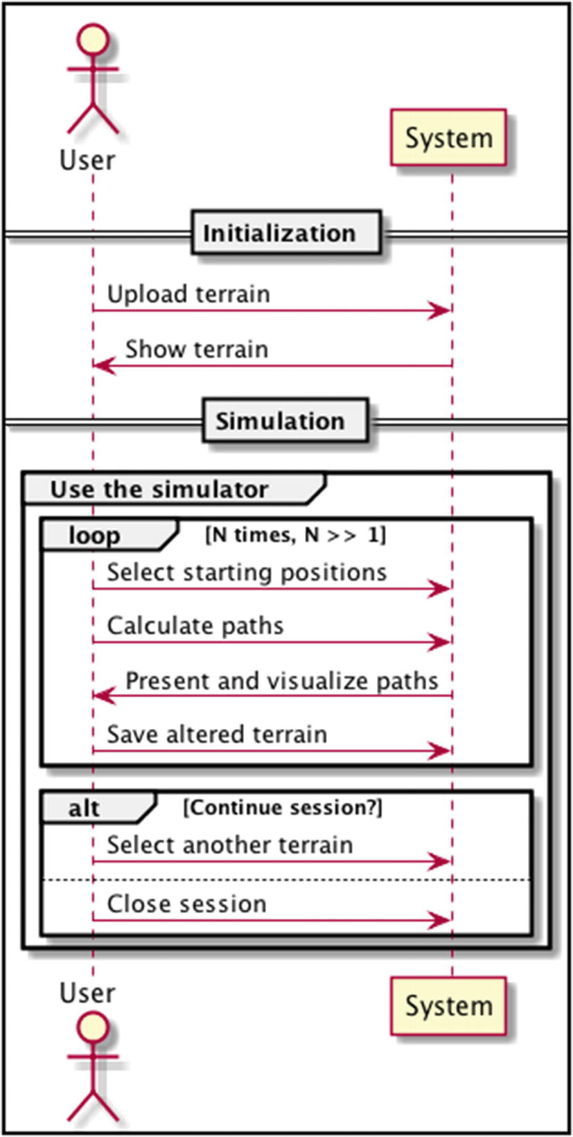
This sequence of interaction will happen independently for each user

We assume and optimize for a situation where the number of trials per terrain is large (>> 1). This may have a negative impact on extreme cases of 1 simulation per terrain. Again, this is a fine example of why you should be clear about your use cases.

There are three tactics to optimize a program:
  • Eliminate or reduce the number of calls to methods.

  • Speed up methods.

  • Combine the previous two options.

Obviously, a tremendous number of calls target the terrain property and wall method. These calls solely happen from the next_neighbor method, which is called once for each point in a path. If calculating a next point would become computationally demanding in the future, then we could eliminate the need to “recalculate” the terrain over and over again by preprocessing it during initialization (see Figure 5-6). Afterward, we would just pick up the next points by interrogating the index. In some sense, you can think of this as a sort of memoization. Figure 5-7 depicts the idea visually. Of course, the drawback is extra memory usage to store preprocessed stuff. Clearly, doing this is only beneficial if there are many simulations over the same terrain and their real-time processing is expensive. Otherwise, it is a total waste of time and memory. We will only speed up the next_neighbor method and leave preprocessing as an additional exercise.
../images/473947_1_En_5_Chapter/473947_1_En_5_Fig7_HTML.jpg
Figure 5-7

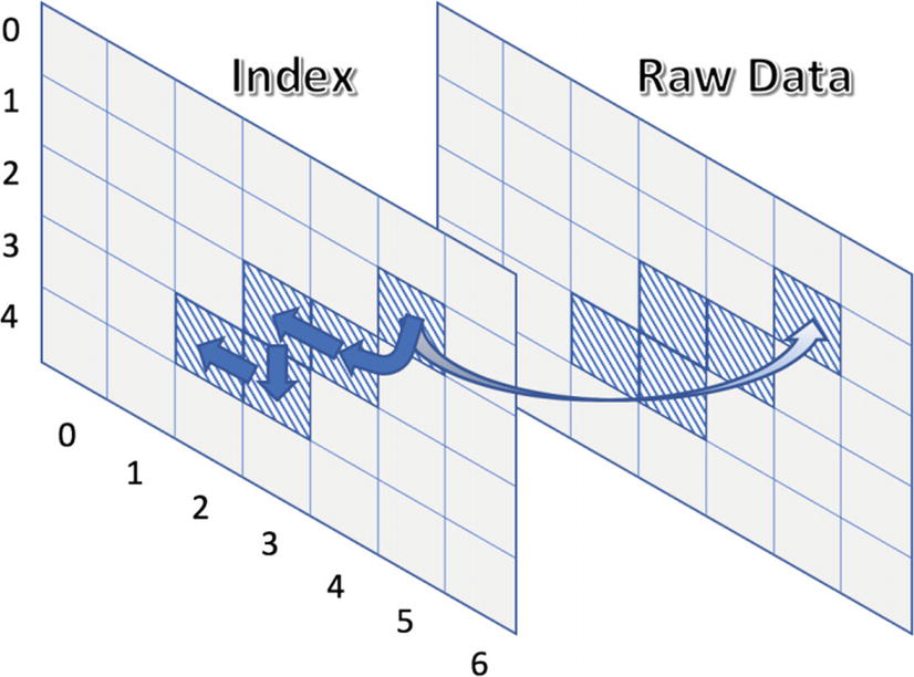
Here, the raw terrain data isn’t used at all during simulation

The next_neighbor method simply reads out next points based upon the current position. Preprocessing is performed by going over every point and storing its best neighbor (it may also be the current point if the ball cannot go anywhere else). For example, the index cell (1, 5) references the next neighbor, whose value is (2, 4). Reading the raw terrain data at (1, 5) yields that point’s altitude and slope.

The find_path method is called as many times as there are starting positions in the list. If we may parallelize find_path executions, then we may decrease the find_paths method’s execution time.

All in all, we have a plan and we are ready for implementation. At this moment, we must rethink how to proceed with construction from the viewpoint of reuse. We definitely should rely on some mature framework, as the realm of parallel and distributed computing is abundant with offerings. Here are our requirements that we expect from the new framework:
  • It must support both explicit and implicit parallelism. So, we are not looking solely for an abstraction over which we can reach out to many cores or machines. For example, Apache Spark exposes a straightforward model through the resilient distributed dataset abstraction but forces us to formulate problems in a specific way. For arbitrarily complex logic, we would need something more akin to generic frameworks, like multiprocessing in Python.

  • We don’t want to rewrite much of the existing code nor depart into another run-time environment. For example, a JVM-based technology isn’t preferable.

  • Preferably, we would like to retain the current APIs when working with new abstractions. This would also reduce learning time.

It turns out that there is an open-source framework that meets our aspirations. Numba (see http://numba.pydata.org ) is a just-in-time (JIT) compiler that translates Python functions with Numpy code into machine code. There is no special precompilation phase. All you need to do is annotate functions that you wish to accelerate. Numba integrates seamlessly with Dask and may even produce universal functions that behave like built-in Numpy functions. Being able to speed up arbitrary functions is very important when you have complex business logic with lots of conditionals. In this case, any crude parallelization scheme would become cumbersome to apply. Finally, with Numba you can optimize for GPUs, again something very crucial to gain top performance.

Listing 5-11 shows the new ParallelSimplePathFinder class . It uses the logic of the inherited next_neighhbor method to create an index, so the ball movement rules remain intact. All that was required to boost performance is that single decorator. Of course, you need to know the constraints regarding content of jit decorated functions. This is why you should always keep nopython=True set (otherwise you will not get warnings).
"""Efficient parallel version of the path finder system."""
from typing import Tuple, Set
import numpy as np
from numba import jit
from pathfinder.non_recursive_simple_pathfinder import NonRecursiveSimplePathFinder
class ParallelSimplePathFinder(NonRecursiveSimplePathFinder):
    """Concrete path finder that uses Numba to perform operations in parallel."""
    @staticmethod
    @jit(nopython=True, parallel=True, cache=True)
    def _best_neighbor(terrain: np.ndarray, position: Tuple[int, int]) -> Tuple[int, int]:
        curr_x, curr_y = position
        length, width = terrain.shape[:2]
        current_slope = terrain[position][1]
        min_altitude = terrain[position][0]
        min_position = position
        for delta_x in range(-1, 2):
            for delta_y in range(-1, 2):
                new_position = (curr_x + delta_x, curr_y + delta_y)
                new_x, new_y = new_position
                if not ((new_x < 0) or
                        (new_y < 0) or
                        (new_x >= length) or
                        (new_y >= width)) and not new_position == position:
                    new_altitude = terrain[new_position][0]
                    if new_altitude < min_altitude or (new_altitude == min_altitude and
                                           current_slope > 0):
                        min_altitude = new_altitude
                        min_position = new_position
        return min_position
    def next_neighbor(self, position: Tuple[int, int],
                      visited: Set[Tuple[int, int]]) -> Tuple[int, int]:
        """
        Uses a vectorized clockwise search of neighbors starting at south-west.
        Example:
        >>> terrain = np.array([[(-2, 0), (2, 0), (2, 1), (3, 1)]])
        >>> path_finder = ParallelSimplePathFinder(terrain)
        >>> path_finder.next_neighbor((0, 2), set((0, 2)))
        (0, 1)
        """
        best_neighbor = ParallelSimplePathFinder._best_neighbor(self.terrain, position)
        if not best_neighbor in visited:
            return best_neighbor
        return position
if __name__ == "__main__":
    import doctest
    doctest.testmod()
Listing 5-11

Performance-Tuned Path Finder Class That Uses Numba

Let’s now repeat the command that we used in the baseline version (the path_finder variable points to our new class):
>> %time calc_paths = path_finder.find_paths([(0, 0), (1000, 1000)])
CPU times: user 8.42 s, sys: 395 ms, total: 8.82 s
Wall time: 8.81 s

So, execution time went down from 1min 46s to 8.82s! This is more than a 10× improvement. The good news is that there are tons of more possibilities to decrease the running time (indexing, mentioned earlier, is one of them).

Retrospective of Version 1.3

This version was intended to show you how a properly structured code base helps evolution. We made small modifications in each increment, without spending time to fight clutter. The Python world is abundant with frameworks that wait to be reused. You must avoid the danger of being unduly influenced by any of them. To ensure that your program is always amenable to additional enhancements, you must control and assess what it requires to operate efficiently and avoid adding functionality that has dependencies. This concludes our series of iterations regarding this project. Figure 5-8 shows the radar diagram for this last version.
../images/473947_1_En_5_Chapter/473947_1_En_5_Fig8_HTML.jpg
Figure 5-8

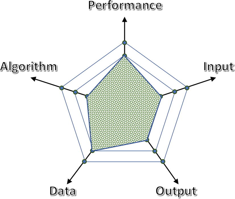
The performance is now satisfactory, which allows us to add new, complex features

Abstractions vs. Latent Features

Thus far, we have worked with software abstractions: frameworks, classes, data structures, etc. Abstractions are our principal mechanism to combat complexity. Working with entities on proper abstraction levels increases both efficacy and quality. These software abstractions have all been explicit, because we created them. In this section you will see that there is a totally different category of abstractions that emerges behind the scenes. We don’t even know what they represent, although we know everything about the process responsible for their creation. Often these artifacts are called latent features .

Latent features describe raw data in a more concise fashion; by using them, we can achieve high compression in many aspects. Besides dropping the sheer data size, more importantly, we can reduce the number of dimensions in the dataset. This directly brings down complexity, as many machine-learning algorithms work much better in lower dimensional space (we will talk about machine learning in Chapter 7).

There are two fundamental compression procedures: fully explainable and partially explainable. In Chapter 2 you witnessed the former, where the application of mathematical statistics produced a more compact data representation. In other words, we summarized the dataset while preserving all pertinent details regarding customer behavior. In this section, you will see an example of partially explainable compression procedures.

Interpretability of your solution is a very important topic nowadays (see reference [1] for a good recount). For example, many companies want to know how and why particular items were recommended to users by a recommender system. You cannot just respond that it was decided by a machine that leverages a well-known matrix factorization technique. Remember this side-effect of latent features when you start to design a new system.

Compressing the Ratings Matrix

Suppose that you are building a recommender system and store ratings of users for items inside matrix R. Each row represents one user and each column represents an item. For user u and item i you can easily find out the rating rui by looking at the corresponding cell of the matrix. Obviously, may cells will be empty, because users will rate only a miniscule number of items. With millions of users and items, this matrix may become enormous (even if you store it as a sparse matrix). Apparently, no commercial recommender system uses such raw matrices.

There is a theorem of linear algebra stating that any matrix Rmxn with rank k can be decomposed into three subordinate matrices Umxk, Skxk, and Vkxn, such that R = USVT. The columns of U and V are pairwise orthogonal, and the matrix S is diagonal (its elements are called singular values). Now, the magic is related to choosing the number of latent features d < k, so that we can abandon most of the elements in U, S, and V. Of course, the goal is to still be able to approximately reconstruct the original matrix R. The aim is to efficiently calculate predictions of ratings for users and items that haven’t been rated (we presume a multivalued rating scheme, such as number of stars).1

The following snippet from Spyder’s console creates a random dense ratings matrix R, factorizes it into subordinate matrices, and demonstrates what happens in a lower dimensional case (when d < rank(R)):
>> m = 10, n = 6
>> np.random.seed(10)
>> a = np.random.randint(1, 5, size=(m, n))
>> a
array([[2, 2, 1, 4, 1, 2],
       [4, 1, 2, 2, 1, 2],
       [2, 3, 1, 2, 1, 3],
       [1, 3, 1, 4, 1, 1],
       [4, 4, 3, 1, 4, 3],
       [3, 2, 1, 1, 3, 2],
       [4, 3, 2, 2, 2, 4],
       [2, 3, 2, 1, 3, 3],
       [3, 2, 1, 2, 4, 2],
       [1, 4, 3, 2, 2, 3]])
>>
>> np.linalg.matrix_rank(a)
6
>>
>> u, s, vt = np.linalg.svd(a, full_matrices=True)
>> u.shape, s.shape, vt.shape
((10, 10), (6,), (6, 6))
>>
>> s
array([18.30683743,  4.73046021,  3.60649612,  2.79133251,  1.65155672, 0.97798699])
>>
>> np.allclose(a, np.dot(u[:, :n] ∗ s, vt))
True
>>
>> d = 5
>> np.allclose(a, np.dot(u[:, :d] ∗ s[:d], vt[:d]))
False
>>
>> np.allclose(a, np.dot(u[:, :d] ∗ s[:d], vt[:d]), atol = 0.3)
True
>>
>> u[:1, :d]
array([[-0.26299616, -0.50400408,  0.2691205 ,  0.10395761,  0.06633331]])

The singular values are ordered in descending order, and we kept the first five latent features. Sure, we no longer can faithfully reconstruct R in a lower dimensional space, but we may estimate its values quite correctly. Ratings anyhow contain noise, and our goal isn’t to figure out the known values. The mission is to predict unknown ratings, and for this purpose an approximation of R is good enough. The last line above shows the reduced vector for user 1. It is expressed with five latent features that somehow designate the “taste” of users. Without further deep analysis, we have no inkling what aspect of “taste” they denote.

This example only scratches the surface of recommender systems, but I hope that you have grasped the key idea.2 You will encounter latent features everywhere; the principal component analysis method and neural networks are all based upon them. In some sense, instead of doing feature engineering yourself, you leave this job to a machine.

Exercise 5-1. Random Path Finder

The SimplePathFinder class visits potential neighbors in a predefined order. Consequently, it will generate the same path every time (assuming no change in the starting position). This doesn’t quite mimic the real world and is also a boring behavior.

Create a new class RandomSimplePathFinder as a child of SimplePathFinder and override the next_neighbor method. It should randomly select the next point among equally good candidates, if there is more than one. Feel free to refactor the parent class(es), if you judge that would reduce duplication of code.

Exercise 5-2. Mores Reusable Interaction Monitor

The InteractionMonitor class accepts a text area to update its value property each time a user selects a new starting position. This was OK for our purpose but may be inadequate in other situations.

Improve this class by making it more reusable. One option is to receive a function (instead of that informational area) accepting one tuple argument that denotes the selected starting position. In this manner, users could have full control over the selection process. One good use case is selecting multiple points. These could be collected by your custom function until the desired number of points is reached. Afterward, your function would call the stop method on the InteractionMonitor instance.

Summary

This chapter has demonstrated how software engineering methods and concepts interplay with those related specifically to data science. You have witnessed how progression through multiple interrelated dimensions requires careful planning and realization. These dimensions were performance, input, output, data, and algorithms. Radar diagrams are very handy to keep you organized and to visually represent strengths and weaknesses of the current system. You should have implicitly picked up the main message: as soon as you start doing something advanced in any particular area, things get messy. This is the principal reason why methods that work at a small scale don’t necessarily work in large-scale situations.

There are tons of frameworks that we haven’t even mentioned, but all of them should be treated similarly to how we treated Numba in this chapter. The next two paragraphs briefly introduce a few notable frameworks, and in upcoming chapters you will encounter some very powerful frameworks, such as PyTorch for deep neural networks (in Chapter 12). We will also come back to Dask in Chapter 11.

Dask (see https://dask.org ) is a library for parallel computing in Python (consult references [1] and [2] for a superb overview). Dask parallelizes the numeric Python ecosystem, including Numpy, Pandas, and Scikit-Learn. You can utilize both the implicit and explicit parallelization capabilities of Dask. Furthermore, Dask manages data that cannot fit into memory as well as scales computation to run inside a distributed cluster. Dask introduces new abstractions that mimic the APIs of the underlying entities from the SciPy ecosystem. For example, with dask arrays you can handle multiple smaller Numpy arrays in the background while using the familiar Numpy API. There are some gotchas you need to be aware of. For example, don’t try to slice large dask arrays using the vindex method (implements fancy indexing over dask arrays). At any rate, combining Dask and Numba can give you a very powerful ensemble to scale your data science products.

Luigi (see https://github.com/spotify/luigi ) is a framework to build complex pipelines of batch jobs with built-in Hadoop support (this represents that harmonizing power between various frameworks). On the other hand, Apache Nifi (see https://nifi.apache.org ) is useful to produce scalable data pipelines. As you can see, these two frameworks attack different problems, although they may be orchestrated to work together depending on your needs.

References

  1. 1.

    Steven Strogatz, “One Giant Step for a Chess-Playing Machine,” New York Times, https://www.nytimes.com/2018/12/26/science/chess-artificial-intelligence.html , Dec. 26, 2018.

     
  2. 2.

    Matthew Rocklin, “Scaling Python with Dask,” Anaconda webinar recorded May 30, 2018, available at https://​know.​anaconda.​com/​Scaling-Python-Dask-on-demand-registration.​html.

     
  3. 3.
     
..................Content has been hidden....................

You can't read the all page of ebook, please click here login for view all page.
Reset
3.145.73.193