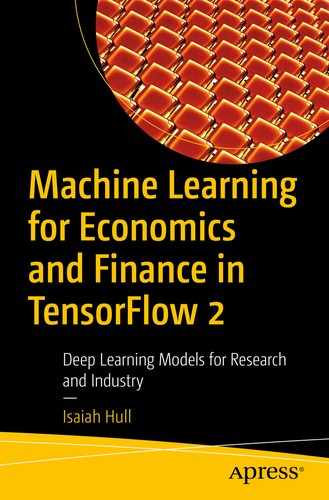
Comparison of discriminator and generator models
Thus far, we have focused on discriminative models in this book; however, there was one exception: the latent Dirichlet allocation (Blei et al. 2003), which we introduced in Chapter 6. The LDA model took a text corpus as an input and returned a set of topics, where each topic was defined as a distribution over the vocabulary.
There has recently been considerable progress in the generative machine learning literature, and much of it has been concentrated in the development of two types of models: variational autoencoders (VAEs) and generative adversarial networks (GANs). With respect to image, text, and music generation, these two categories of model have delivered considerable breakthroughs.
For the most part, this progress hasn’t yet reached the economics and finance disciplines; however, some work in economics has begun to make use of GANs. In the final section of the chapter, we will briefly discuss two recent applications of GANs in economics (Athey et. al. 2019 and Kaji et al. 2018) and speculate on potential future uses.
Variational Autoencoders
In Chapter 8, we introduced the concept of an autoencoder, which consisted of two networks with shared weights: an encoder and a decoder. The encoder transformed the model inputs into a latent state. The decoder took the latent state as an input and produced a reconstruction of the features input into the encoder. We trained the model by computing a reconstruction loss, which was a transformation of the difference between the inputs and their predicted values.
- 1.
The location and distribution of latent states: The latent states of an autoencoder with N nodes are points in ℝN. For many problems, these points will tend to cluster in the same area; however, the autoencoder does not allow us to explicitly determine how and where such points cluster in ℝN. This might seem unimportant, but it will ultimately determine what latent states can be fed into the model. If, for instance, we are attempting to generate an image, it would be useful to know what constitutes a valid latent state and, thus, what can be fed into the model. Otherwise, we will use states that are far away from anything the model has observed, which will yield a novel, but perhaps unconvincing image.
- 2.
The performance of latent states not present in training: An autoencoder is trained to reconstruct inputs for a set of examples. For the latent state associated with a set of features, the decoder should yield outputs that resemble the input features. If, however, we perturb the latent vector slightly, there’s no guarantee that the decoder will have the capacity to generate a convincing example from a point it has never visited.
Variational autoencoders (VAEs) were developed to overcome these limitations. Rather than having a latent state layer, VAEs have a mean layer, a log variance layer, and sampling layer. The sampling layer draws from a normal distribution defined by the mean and log variance parameters in the preceding layers. The output of the sampling layer is then passed to the decoder as the latent state during the training process. Passing the same features to the encoder twice will yield different latent states each time.
Beyond the differences in architecture, VAEs also modify the loss function to include the Kullback-Leibler (KL) divergence for each normal distribution in the sampling layer. The KL divergence penalizes the distance between each of the normal distributions and a normal distribution with both a mean and log variance of zero.
The combination of these features accomplishes three things. First, it eliminates the determinism of latent states. Each set of features will now be associated with a distribution of latent states, rather than a single latent state. This will tend to improve generative performance by forcing the model to treat each individual latent state feature as a continuous variable. Second, it eliminates the sampling problem. We can now draw valid states randomly by making use of the sampling layer. And third, it corrects the issue with the latent distribution in space. The KL divergence component of the loss will push the distribution means close to zero and force them to have similar variances.
The remainder of this section will focus on the implementation of VAEs in TensorFlow. For an extended overview of the development of VAE models and a detailed exploration of their theoretical properties, see Kingma and Welling (2019).
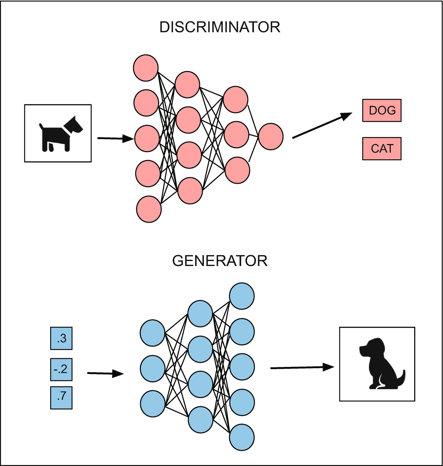
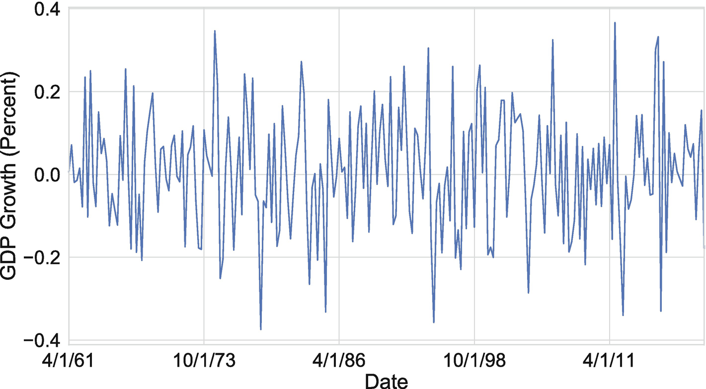
The example we’ll use in this chapter makes use of the GDP growth data we introduced in Chapter 8. As a refresher, it consisted of quarterly time series that spanned the period between 1961:Q2 and 2020:Q1 for 25 different OECD countries. In Chapter 8, we used dimensionality-reduction techniques to extract a small number of common components from the 25 series at each point in time.
Prepare GDP growth data for use in a VAE
Define function to perform sampling task in VAE
Notice that the sampling layer does not contain any parameters of its own. Rather, it takes a pair of parameters as inputs, draws epsilon from a standard normal distribution for each output node in the latent state, and then transforms each draw using the mean and lvar parameters that correspond to the nodes in that state.
Once we have defined a sampling layer, we can also define an encoder model, which will closely resemble the one we constructed for the autoencoder model. We’ll do this in Listing 9-3. The only initial difference is that we’ll take the full time series for a country as an input, rather than the cross-section of values across countries at a point in time.
Another difference appears in the mean and lvar layers, which were not present in the autoencoder. These layers have the same number of nodes as the latent state. This is because they consist of mean and log variance parameter values for normal distributions that are associated with each of the nodes in the latent state.
Define encoder model for VAE
In Listing 9-4, we’ll define functional models for the decoder model and the entire variational autoencoder. Similar to the decoder component of an autoencoder, it accepts the latent state as an input from the encoder and then produces a reconstruction of the inputs as an output. The full VAE model also bears similarity to an autoencoder, taking a time series as an input and transforming it into a reconstruction of the same time series.
Define decoder model for VAE
Define VAE loss
Compile and fit VAE
Generate latent states and time series with trained VAE.
VAE-generated time series for GDP growth for the United States
While this example was simple and the latent state contained only two nodes for the purpose of demonstration, the VAE architecture can be applied to a wide variety of problems. We can, for instance, add convolutional layers to the encoder and decoder and change the input and output shapes. That will give us a VAE that generates images. Alternatively, we could add LSTM cells to the encoder and encoder, which would give us a VAE that could generate text or music.1 Furthermore, an LSTM-based architecture could yield some improvements in time series generation over the dense network approach we adopted in this example.
Generative Adversarial Networks
Two families of models have dominated the generative machine learning literature: variational autoencoders and generative adversarial networks. VAEs, as we’ve seen, provide granular control over the generation of examples through the manipulation of latent states and the features they encode. GANs, in contrast, have been more successful at producing highly convincing examples of classes. For example, some of the most convincing generated images are produced using GANs.
As we discussed in the previous section, VAEs are a combination of two models: an encoder and a decoder, joined by a sampling layer. Similarly, GANs also consist of two models: a generator and a discriminator. The generator takes a random input vector, which we may think of as a latent state, and generates an example of a class, such as a real GDP growth time series (or an image, a sentence, or a musical score).
Once the generator component of a GAN has produced several examples of a class, they are passed to the discriminator, along with an equal number of true examples. In our case, this would be a combination of true and generated real GDP growth series. The discriminator is then trained to differentiate between the real and fake examples.
After the discriminator has finished the classification task, we can train the generator using an adversarial network, which combines both the generator and discriminator models. Just as was the case for the encoder and decoder components of the VAE, an adversarial network will share weights with both networks. The adversarial network will train the generator to maximize the loss of the discriminator network.
As Goodfellow et al. (2017) discuss, we may view the two networks as trying to maximize their respective payoffs in a zero sum game, where the discriminator receives v(g, d) and the generator receives −v(g, d). The generator chooses samples, g, to trick the discriminator; and the discriminator chooses probabilities, d, for each of those samples. The equilibrium, characterized by a set of generated images, g∗, is given in Equation 9-1.

Consequently, when we train the adversarial part of the network, we must freeze the discriminator weights. This will constrain the network to improve the generation process, rather than weakening the discriminator. Iterating over these steps in the training process will ultimately yield the evolutionary equilibrium described in Equation 9-1.
Figure 9-3 illustrates the generator and discriminator networks of a GAN. To summarize, the generator yields novel examples, which are not drawn from the data. The discriminator combines those examples with true examples and then performs classification. And the adversarial network trains the generator by attaching it to a discriminator, but with frozen weights. Training over the network occurs iteratively.

Depiction of the generator and discriminator from a GAN
Prepare GDP growth data for use in a GAN
In Listing 9-9, we define the generative model. We again follow the simple VAE model and draw a vector with two elements as an input to the generator. Since the input to the generator can be seen as an analogy to the latent vector in a VAE, we should view the generator as a decoder. This means we’ll start with a narrow, bottleneck-type layer and will upsample to the output, which will be a generated GDP growth time series.
Define the generative model of a GAN
Define and compile the discriminator model of a GAN
We have now defined a generator model and a discriminator model. We have also compiled the discriminator. The next step is to define and compile an adversarial model, which will be used to train the generator. The adversarial model will share weights with the generator and will use a frozen version of the weights for the discriminator – that is, the weights will not update when we train the adversarial network, but they will update when we train the discriminator.
Define and compile the adversarial model of a GAN
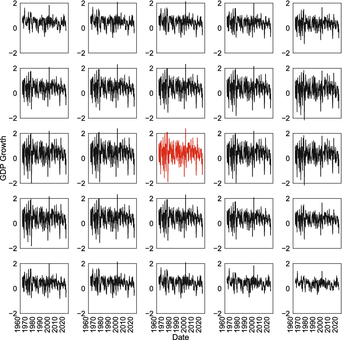
Train the discriminator and the adversarial network
We start by defining the batch size. We then enter the training loop, which consists of several steps. First, we draw random integers and use them to select rows in the GDP matrix, which each consists of a GDP growth time series. This will be the real samples in the discriminator’s training set. Next, we generate the fake data by drawing latent vectors and then passing them to generator. We then combine both types of series and assign them the corresponding labels (i.e., 1 = real and 0 = fake). We can now pass this data to the discriminator to perform a single batch of training.
We next perform an iteration of training for the adversarial network. Here, we’ll generate a batch of latent states, input them into generator, and then train with the objective of tricking the discriminator into classifying them as real. Notice that we’re iterating over the training of two models and won’t use normal stopping criteria for the training process. Rather, we will look for a stable evolutionary equilibrium where neither model appears to be able to gain an advantage.
Discriminator and adversarial model losses by training iteration
Example fake GDP growth series
Applications in Economics and Finance
Throughout this chapter, we concentrated on what might seem like an obscure example: generating simulated GDP growth series through the use of generative machine learning models; however, such exercises are common in Monte Carlo simulation studies, which are used to test the small sample properties of estimators in econometrics. Without generating realistic series and adequately capturing interdependencies between series, it is challenging to accurately evaluate the properties of estimators.
In fact, one of the earliest applications of GANs in the economics literature was intended to achieve precisely this objective. Athey et al. (2019) consider the possibility of using Wasserstein GANs to simulate data that appears similar to observations from an existing dataset that is insufficiently large to be used in a Monte Carlo simulation. The value of this is that it allows an econometrician to avoid the two common alternatives to this approach: (1) drawing randomly from the small dataset itself, which will result in many repetitions of the same observations, and (2) generating simulated series that typically fail to accurately capture dependencies between series in the dataset. Athey et al. (2019) demonstrate the value of their approach (and GANs more generally) by evaluating estimators using artificial data generated by a WGAN.
In addition to Athey et al. (2019), recent work in the economics literature (Kaji et al. 2018) examines whether WGANs can be used to perform indirect inference, which is typically used to estimate structural models in economics and finance. In Kaji et al. (2018), they attempt to estimate a model in which workers of different types are choosing from a wage and location menu. The parameters they want to recover are structural and cannot be directly estimated from the data, which requires them to use an indirect inference method. The approach they use is to couple model simulation with a discriminator, training the model until the simulated data is indistinguishable from the true data.
Beyond the existing applications, which are currently focused on model estimation, GANs and VAEs could also be used in off-the-shelf applications to image and text generation. While the use of image data remains limited in economics – even in discriminative models – GANs and VAEs offer the possibility of performing visual counterfactual simulations with economic data. In urban economics, for instance, we could infer how the placement of public infrastructure would have changed depending on the state of public policy and other factors.
Similarly, the growing natural language processing literature in economics and finance could make use of text generation to examine how, for instance, company press releases would differ when the underlying state of the economy or state of the industry changes.
Summary
Prior to this chapter, this book primarily discussed discriminative machine learning models. Such models perform classification or regression. That is, they take features from a training set and attempt to discriminate between different classes or make a continuous prediction for a target. Generative machine learning differs from discriminative machine learning, in that it generates new examples, rather than discriminating among examples.
Outside of the economics and finance disciplines, generative machine learning has been used to create compelling images, music, and text. It has also been used to improve Monte Carlo simulation (Athey et al. 2019) and perform indirect inference for structural models (Kaji et al. 2018) in economics.
In this chapter, we focused on two generative models: the variational autoencoder (VAE) and the generative adversarial network (GAN). The VAE model extended the autoencoder by including mean, variance, and sampling layers. This improved the autoencoder by imposing restrictions on its latent space, forcing states to cluster around the origin and have a log variance of 0.
Similar to autoencoders and VAEs, GANs also consist of multiple component models: a generator model, a discriminator model, and an adversarial model. The generator model creates novel examples. The discriminator model attempts to classify them. And the adversarial model trains the generator to create compelling examples that trick the discriminator. The training process for GANs involves finding a stable evolutionary equilibrium.
Finally, we demonstrated how both VAEs and GANs can be used to generate artificial GDP growth data. We also discussed how they are being applied within economics currently and how they might be applied in the future if they gain more widespread adoption.
Bibliography
Athey, S., G.W. Imbens, J. Metzger, and E. Munro. 2019. “Using Wasserstein Generative Adversarial Networks for the Design of Monte Carlo Simulations.” Working Paper No. 3824.
Blei, D.M., A.Y. Ng, and M.I. Jordan. 2003. “Latent Dirichlet Allocation.” Journal of Machine Learning Research 3 (993–1022).
Goodfellow, I., Y. Bengio, and A. Courville. 2017. Deep Learning. Cambridge, MA: MIT Press.
Goodfellow, I.J., J. Pouget-Abadie, M. Mirza, B. Xu, D. Warde-Farley, S. Ozair, A. Courville, and Y. Bengio. n.d. “Generative adversarial networks.” NIPS’2014. 2014.
Kaji, T., E. Manresa, and G. Pouliot. 2018. “Deep Inference: Artificial Intelligence for Structural Estimation.” Working Paper.
Kingma, D.P., and M. Welling. 2019. “An Introduction to Variational Autoencoders.” Foundations and Trends in Machine Learning 12 (4): 307–392.
Krohn, J., G. Beyleveld, and A. Bassens. 2020. Deep Learning Illustrated: A Visual, Interactive Guide to Artificial Intelligence. Addison-Wesley.