The term “regression” differs in common usage between econometrics and machine learning. In econometrics, a regression involves the estimation of parameter values that relate a dependent variable to independent variables. The most common form of regression in econometrics is multiple linear regression, which involves the estimation of a linear association between a continuous dependent variable and multiple independent variables. Within econometrics, however, the term also encompasses non-linear models and models where the dependent variable is discrete. To the contrary, a regression in machine learning refers to a linear or non-linear supervised learning model with a continuous dependent variable (target). Throughout this chapter, we will adopt the broader econometrics definition of regression, but will introduce methods commonly applied in machine learning.
Linear Regression
In this section, we’ll introduce the concept of a “linear regression,” which is the most commonly employed empirical method in econometrics. It is used when the dependent variable is continuous, and the true relationships between the dependent variable and the independent variables are assumed to be linear.
Overview
A linear regression models the relationship between a dependent variable, Y, and a set of independent variables, {X0, …, Xk}, under the assumption of linearity in the coefficients. Linearity requires that the relationship between each Xj and Y can be modeled as a constant slope, represented by a scalar coefficient, βj. Equation 3-1 provides the general form for a linear model with k independent variables.

In many cases, we will adopt the notation given in Equation 3-2, which explicitly specifies an index for each observation. Yi, for instance, denotes the value of variable Y for entity i.

In addition to entity indices, we will often use time indices in economic problems. In such cases, we will typically use a t subscript to indicate the time period in which the variable is observed, as we have done in Equation 3-3.

In a linear regression, the model parameters, {α, β1, …, βk}, do not vary with time or by entity and, thus, are not indexed by either. Additionally, non-linear transformations of the parameters are not permitted. A dense neural network layer, for instance, has a similar functional form, but applies a non-linear transformation to the sum of coefficient-variable products, as shown in Equation 3-4, where σ represents the sigmoid function.

While linearity may appear to be a severe functional form restriction, it does not prevent us from applying transformations – including non-linear transformations – to the independent variables. We can, for instance, re-define X0 as its natural logarithm and include it as an independent variable. Linear regressions also permit interactions between two variables, such as X0 ∗ X1, or indicator variables, such as  . Additionally, in time series and panel settings, we can include lags of variables, such as Xt − 1j and Xt − 2j.
Transforming and re-defining variables makes linear regression a flexible method that can be used to approximate non-linear functions to an arbitrarily high degree of precision. For instance, consider the case where the true relationship between X and Y is given by the exponential function in Equation 3-5.

If we take the natural logarithm of Yi, we can perform the linear regression in Equation 3-6 to recover the model parameters, {α, β}.

In most settings, we won’t know the underlying data generating process (DGP). Furthermore, there will not be a deterministic relationship between the dependent variable and independent variables. Rather, there will be some noise, ϵi, associated with each observation, which could arise as the result of unobserved, random differences across entities or measurement error.
As an example of this, let’s say that we have data drawn from a process that is known to be non-linear, but its exact functional form is unknown. Figure 3-1 shows a scatterplot of the data, along with plots of two linear regression models. The first is trained under the assumption that the relationship between X and Y is well-approximated over the [0, 10] interval using a single line, as in Equation 3-7. The second is trained under the assumption that five line segments are needed, as in Equation 3-8.


Two linear approximations of a non-linear function
Figure 3-1 suggests that using a linear regression model with a single slope and intercept was insufficient; however, using multiple line segments in the form of a piecewise polynomial spline was sufficient to approximate the non-linear function, even though we worked entirely within the framework of linear regression.
Ordinary Least Squares (OLS)
Linear regression , as we have seen, is a versatile method that can be used to model the relationship between a dependent variable and set of independent variables. Even when that relationship is non-linear, we saw that it was possible to approximate it in a linear model using indicator functions, variable interactions, or variable transformations. In some cases, we were even able to capture it exactly through a variable transformation.
In this section, we’ll discuss how to implement a linear regression in TensorFlow. The way in which we do this will depend on our choice of loss function. In economics, the most common loss function is the sum or mean of the squared errors, which we will consider first. For the purpose of this example, we will stack all of the independent variables in an n x k matrix, X, where n is the number of observations and k is the number of independent variables, including the constant (bias) term.
We will let  denote the vector of estimated coefficients on the independent variables, which we distinguish from the true parameter values, β. The “error” term that we will use to construct our loss function is given in Equation 3-9. It will often be referred to by different names, such as error, residual, or disturbance term.

Note that ϵ is an n-element column vector. This means that we can square and sum each element by pre-multiplying by its transpose, as in Equation 3-10, which gives us the sum of squared errors.

One of the benefits of using the sum of squared errors as a loss function
– also called performing “ordinary least squares” (OLS) – is that it permits an analytical solution, as derived in Equation 3-11, which means that we do not need to use time-consuming and error-prone optimization algorithms. We obtain this solution by choosing  to minimize the sum of squared errors.


 is a minimum or a maximum. It will be a minimum whenever X has “full rank.” This will hold if no column of X is a linear combination of one or more other columns of X. Listing 3-1 provides a demonstration of how we can perform ordinary least squares (OLS) in TensorFlow for a toy problem
.
is a minimum or a maximum. It will be a minimum whenever X has “full rank.” This will hold if no column of X is a linear combination of one or more other columns of X. Listing 3-1 provides a demonstration of how we can perform ordinary least squares (OLS) in TensorFlow for a toy problem
.Implementation of OLS in TensorFlow 2
For convenience, we have defined the transpose of X as XT. We have also defined XTX as XT post-multiplied by X. We can compute  by inverting XTX, post-multiplying by XT, and then post-multiplying by Y again.
The parameter vector we’ve computed,  , minimizes the sum of squared errors. While computing
  was simple, it might be unclear why we would want to use TensorFlow for such a task. If we had instead used MATLAB, the syntax for writing the linear algebra operations would have been compact and readable. Alternatively, if we had used Stata or any statistics module in Python or R, we’d be able to automatically compute standard errors and confidence intervals for the vector of parameters, as well as measures of fit for the regression.
TensorFlow does, of course, have natural advantages if a task requires parallel or distributed computing; however, the need for this is likely to be minor when performing OLS analytically. The value of TensorFlow will become apparent when we want to minimize a loss function that doesn’t have an analytical solution or when we cannot hold all of the data in memory.
Least Absolute Deviations (LAD)
While OLS is the most commonly used form of linear regression in economics and has many attractive properties, we will sometimes want to use an alternative loss function. We may, for instance, want to minimize the sum of the absolute values of the errors, rather than the sum of the squares. This form of linear regression is referred to as Least Absolute Deviations (LAD) or Least Absolute Errors (LAE).
For all models, including OLS and LAD, the sensitivity of parameter estimates to outliers is driven by the loss function. Since OLS minimizes the squares of errors, it places a high emphasis on setting parameter values to explain outliers. That is, OLS will place a greater emphasis on eliminating a single large error than it will on two errors half of its size. To the contrary, LAD would place equal weight on the large error and the two smaller errors.
Another difference between OLS and LAD is that we cannot express the solution to a LAD regression analytically, since the absolute value prevents us from obtaining a closed-form algebraic expression. This means we must search for the minimum by “training” or “estimating” the model.
While TensorFlow wasn’t particularly useful for solving OLS, it has clear advantages when performing a LAD regression or training another type of model that has no analytical solution. We’ll see how to do this in TensorFlow and also evaluate how accurately TensorFlow identifies the true parameter values at the same time. More specifically, we’ll perform a Monte Carlo experiment, where we randomly generate data under certain assumed parameter values. We’ll then use the data to estimate the model, allowing us to compare the true and estimated parameters.
Listing 3-2 shows how the data is generated. We start by defining the number of observations and number of samples. Since we want to evaluate TensorFlow’s performance, we’ll train the model parameters on 100 separate samples. We’ll also use 10,000 observations to ensure that there is sufficient data to train the model.
Next, we define the true values of the model parameters, alpha and beta, which correspond to the constant (bias) term and the slope. We set the constant term to 1.0 and the slope to 3.0. Since these are the true values of the parameters and do not need to be trained, we will use tf.constant() to define them.
We now draw X and epsilon from normal distributions. For X, we use a standard normal distribution, which has a mean of 0 and a standard deviation of 1. These are the default parameter values for tf.random.normal(), so we do not need to specify anything beyond the number of samples and observations. For epsilon, we use a standard deviation of 0.25, which we specify using the stddev parameter . Finally, we compute the dependent variable, Y.
Generate input data for a linear regression
Listing 3-3 provides the code for the first step in the model training process in TensorFlow. We first draw values from a normal distribution with a mean of 0 and a standard deviation of 5.0 and then use them to initialize alphaHat and betaHat . The choice of 5.0 is arbitrary, but is intended to emulate a problem in which we have limited prior knowledge about the true parameter values. We use the suffix “Hat” to indicate that these are not the true values, but estimates. Since we want to train the parameters to minimize the loss function, we will define them using tf.Variable() , rather than tf.constant().
The next step is to define a function to compute the loss. A LAD regression minimizes the sum of absolute errors, which is equivalent to minimizing the mean absolute error. We will minimize the mean absolute error, since this has better numerical properties.1
Initialize variables and define the loss
Define an optimizer and minimize the loss function
Plot the parameter training histories
Furthermore, alphaHat and betaHat do not appear to adjust any further after they converge on their true parameter values. This suggests that the training process was stable and the stochastic gradient descent algorithm, which we will discuss in detail later in the chapter, was able to identify a clear local minimum, which turned out to be the global minimum in this case.2

History of parameter values over 1000 epochs of training
Parameter estimate counts from Monte Carlo experiment
Other Loss Functions
As we discussed, OLS has an analytical solution, but LAD does not. Since most machine learning models do not permit an analytical solution, LAD can provide an instructive example. The same process we used to construct a model, define a loss function, and perform minimization for LAD will be repeated throughout the chapter and book. Indeed, the steps used to perform LAD can be applied to any form of linear regression by simply modifying the loss function.
There are, of course, reasons to favor OLS beyond the fact that it has a closed-form solution. For instance, if the conditions for the Gauss-Markov Theorem are satisfied, then the OLS estimator has the lowest variance among all linear and unbiased estimators.3 There is also a large econometric literature which builds on OLS and its variants, making it a natural choice for related work.
In many machine learning applications within economics and finance, however, the objective will often be to perform prediction, rather than hypothesis testing . In those cases, it may make sense to use a different form of linear regression; and using TensorFlow will make this task easier.
Partially Linear Models
In many machine learning applications, we will want to model non-linearities in a way that cannot be satisfactorily achieved using a linear regression model, even with the strategies we outlined earlier. This will require us to use a different modeling technique. In this section, we’ll expand the linear model to allow for the inclusion of a non-linear function.
Rather than constructing a purely non-linear model, we’ll start with what’s called a “partially linear model.” Such a model allows for certain independent variables to enter linearly, while others are permitted to enter the model through a non-linear function.
In the context of standard econometric applications, where the objective is typically statistical inference, a partially linear model would usually consist of a single variable of interest, which enters linearly, and a set of controls, which is permitted to enter non-linearly. The objective of such an exercise would be to perform inference on the parameter that enters linearly.
There are, however, econometric challenges to performing valid statistical inference with partially linear models. First, there is an issue with parameter consistency when the variable of interest and the controls are collinear.4 This is addressed in Robinson (1988), which constructs a consistent estimator for such cases.5 Another issue arises when we apply regularization to the non-linear function of controls. If we simply apply the estimator from Robinson (1988), the parameter of interest will be biased. Chernozhukov et al. (2017) demonstrate how to eliminate bias through the use of orthogonalization and sample splitting.
For the purposes of this chapter, we will focus exclusively on the construction and training of a partially linear model for predictive purposes, rather than for statistical inference. In doing so, we will sidestep questions related to consistency and bias and focus on the practical implementation of a training routine in TensorFlow.
We’ll start by defining the model we wish to train in Equation 3-12. Here, β is the vector of coefficients that enter the model linearly, and g(Z) is a non-linear function of the controls.

Similar to the example for LAD, we’ll use a Monte Carlo experiment to evaluate whether we’ve correctly constructed and trained the model in TensorFlow and also to determine whether we are likely to encounter numerical issues, given our sample size and model specification.
In order to perform the Monte Carlo experiment, we’ll need to make specific assumptions about the values of the linear parameters, as well as the functional form of g(). For the sake of simplicity, we’ll assume that there is only one variable of interest, X, and one control, Z, which enters with the functional form exp(θZ). Additionally, the true parameter values are assumed to be α = 1, β = 3, and θ = 0.05.
Generate data for partially linear regression experiment
Initialize variables and compute the loss
Define a loss function for a partially linear regression
Train a partially linear regression model

History of parameter values over 1000 epochs of training
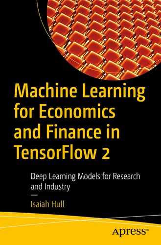
In addition to this, we’ll also examine the estimates for all 100 samples to see how sensitive the results are to the initialization and data. The final epoch parameter values for each sample are visualized in histograms in Figure 3-5. From the figure, it is clear that estimates of both alphaHat and betaHat are tightly clustered around their respective true values. While thetaHat appears unbiased, since the histogram is centered around the true value of theta, there appears to be more variation in the estimates. This suggests that we may want to make adjustments to the training process, possibly by using a higher number of epochs.

Monte Carlo experiment results for partially linear regression
Non-linear Regression
In the previous section, we discussed partially linear models, which had both a linear and non-linear component. Solving a fully non-linear model can be accomplished using the same workflow as the partially linear model. We first generate or load the data. Next, we define the model and loss function. And finally, we instantiate an optimizer and perform minimization of the loss function.
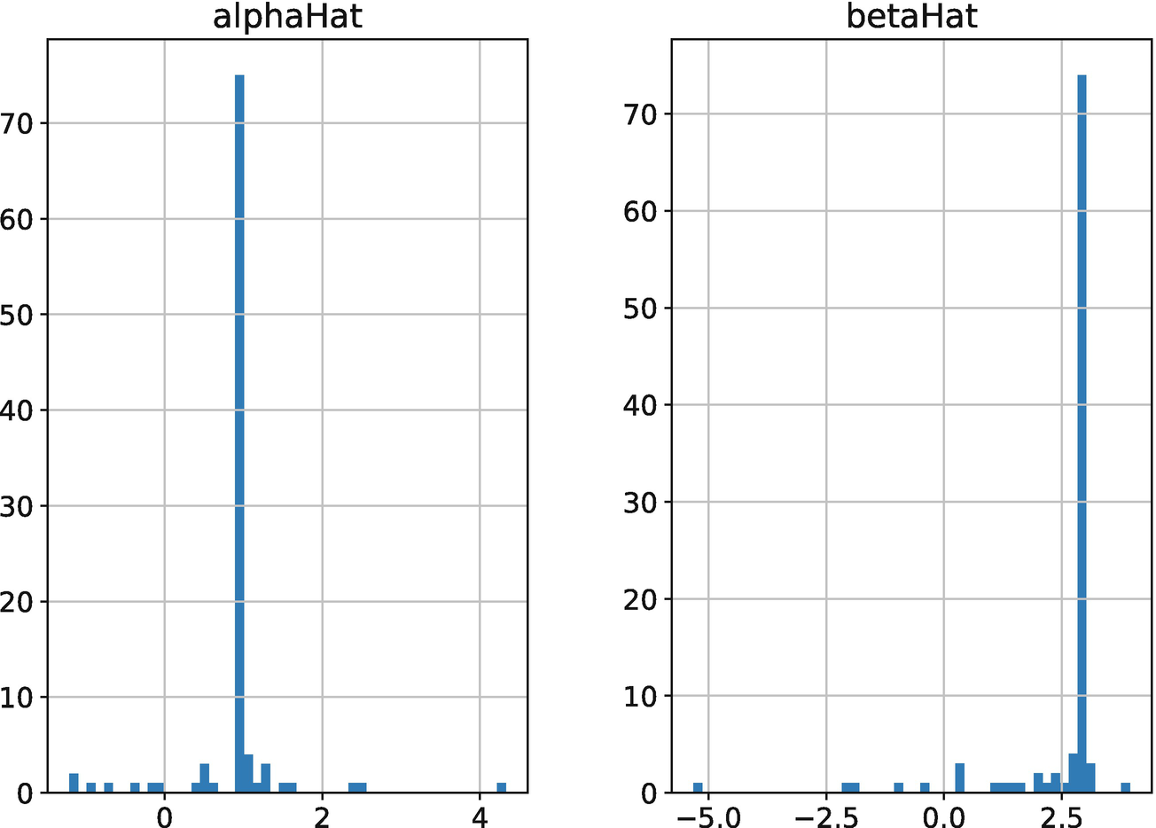
Natural logarithm of the USD-GBP exchange rate at a daily frequency (1970–2020). Source: Federal Reserve Board of Governors
Since exchange rates are challenging to predict, a random walk is often used as the benchmark model in forecasting exercises. As shown in Equation 3-13, a random walk models the next period’s exchange rate as the current period’s exchange rate plus some random noise.

A line of literature that emerged in the 1990s argued that threshold autoregressive (TAR) models could generate improvements over the random walk model. Several variants of such models were proposed, including Smooth Transition Autoregressive Models (STAR) and Exponential Smoothed Autoregressive Models (ESTAR).7
Our exercise will focus on implementing a TAR model in TensorFlow and will deviate from the literature by, among other things, using the nominal, rather than real, exchange rate. Additionally, we will again abstract away from questions related to statistical inference by focusing on prediction.
An autoregressive model assumes that movements in a series are explained by past values of the series and noise. A random walk, for instance, is an autoregressive model of order one – since it contains a single lag – that has an autoregressive parameter of one. The autoregressive parameter is the coefficient on the lagged value of the dependent variable.
A TAR model modifies an autoregression by allowing parameter values to vary according to pre-defined thresholds. That is, parameters are assumed to be fixed within a particular regime, but may vary across regimes. We’ll use the regimes given in Equation 3-14. If there’s a sharp depreciation of more than 2%, then we’re in one regime, associated with one autoregressive parameter value. Otherwise, we’re in another.

Prepare the data for a TAR model of the USD-GBP exchange rate
Define parameters for a TAR model of the USD-GBP exchange rate
Define model and loss function for TAR model of USD-GBP exchange rate
The final step is to define an optimizer and perform optimization, which we do in Listing 3-13.
Train TAR model of the USD-GBP exchange rate

Training history of the TAR model of the USD-GBP exchange rate
We’ve now seen how to perform linear regression with different loss functions, partially linear regression, and non-linear regression in TensorFlow. In the next section, we’ll examine another type of regression, which has a discrete dependent variable.
Logistic Regression
In machine learning , supervised learning models are typically divided into “regression” and “classification” categories based on whether they have a discrete or continuous dependent variable. As discussed earlier, we will use the definition of regression from econometrics, which also applies to classification models, such as a logistic regression.
A logistic regression or “logit” predicts the class of the dependent variable. In a microeconometric setting, a logit might be used to model the choice of transportation over two options. In a financial setting, it might be used to model whether we are in a crisis or not.
Since the process of constructing and training a logistic regression involves many of the same steps as linear, partially linear, and non-linear regression, we will focus exclusively on what differs.
First, the model takes a specific functional form – namely, that of the logistic curve – which is given in Equation 3-15.

Notice that the model’s output is a continuous probability, rather than a discrete outcome. Since probabilities range from 0 to 1, probabilities greater than 0.5 will often be treated as predictions of outcome 1. While this functional form differs from anything we’ve dealt with previously in this chapter, it can be handled using all of the same tools and operations in TensorFlow.
Finally, the other difference between a logistic model and those we’ve defined earlier in this chapter is that it will require a different loss function. Specifically, we will use the binary cross-entropy loss function, which is defined in Equation 3-16.

We use this particular functional form because the outcomes are discrete and the predictions are continuous. Note that the binary cross-entropy loss sums over the product of the outcome variable and the natural log of the predicted probability for each observation. If, for instance, the true class of Yi is 1 and the model predicts a 0.98 probability of class 1, then that observation will add 0.02 to the loss. If, instead, the prediction is 0.10, which is far from the true classification, then the addition to the loss will instead be 2.3.
While computing the binary cross-entropy loss function is relatively simple, TensorFlow simplifies it further by providing the operation tf.losses.binary_crossentropy(), which takes the true label as its first argument and the predicted probability as its second .
Loss Functions
Whenever we solve a model in TensorFlow, we will need to define a loss function. The minimization operation will make use of this function to determine how to adjust parameter values. Fortunately, it will not always be necessary to define a custom loss function. Rather, we will often be able to use one of the pre-defined loss functions provided by TensorFlow.
There are currently two submodules of TensorFlow that contain loss functions: tf.losses and tf.keras.losses. The first submodule contains native TensorFlow implementations of loss functions. The second submodule contains the Keras implementations of the loss functions. Keras is a library for performing deep learning that is available as both a stand-alone module in Python and a high-level API in TensorFlow.
TensorFlow 2.3 offers 15 standard loss functions in the tf.losses submodule . Each of those loss functions takes the form tf.loss_function(y_true, y_pred). That is, we pass the dependent variable, y_true, as the first argument and the model’s predictions, y_pred, as the second argument. It then returns the value of the loss function.
When we work with high-level APIs in TensorFlow in later chapters, we will make use of the loss functions directly. However, for the purpose of this chapter, which is centered around optimization using low-level TensorFlow operations, we will need to wrap those loss functions within a function of the model’s trainable parameters and data. The optimizer will need to make use of the outer function to perform minimization.
Discrete Dependent Variables
The submodule tf.losses offers two loss functions for discrete dependent variables in regression settings: tf.binary_crossentropy(), tf.categorical_crossentropy(), and tf.sparse_categorical_crossentropy(). We have previously covered the binary cross-entropy function, which is used in logistic regression. This provides us with a measure of loss when we have a binary dependent variable, such as an indicator for whether the economy is a recession, and a continuous prediction, such as a probability of being in a recession. For convenience, we repeat the formula for binary cross-entropy in Equation 3-17.

The categorical cross-entropy loss is simply the extension of the binary cross-entropy loss to cases where the dependent variable has more than two categories. Such models are commonly used in discrete choice problems, such as a model of the decision to commute by subway, bicycle, car, or foot. Within machine learning, categorical cross-entropy is the standard loss function for classification problems with more than two classes and is commonly used in neural networks that perform image and text classification. The equation for categorical cross-entropy is given in Equation 3-18. Note that (Yi==k) is a binary variable equal to 1 if Yi is class k and 0 otherwise. Additionally, pk(Xi) is the probability that the model assigns to Xi being class k.

Finally, if we have a problem with a dependent variable that may belong to multiple categories – that is, a “multi-label” problem – we’ll use the sparse categorical cross-entropy loss function, rather than categorical cross-entropy. Notice that the normal cross-entropy loss function assumes that the dependent variable can have only one class.
Continuous Dependent Variables
For continuous dependent variables, the most common loss functions are the mean absolute error (MAE) and mean squared error (MSE). MAE is used in LAD and MSE in OLS. Equation 3-19 defines the MAE loss function, and Equation 3-20 defines the MSE loss. Recall that  is the model’s predicted value for observation i.


Note that we can compute the losses using tf.losses.mae() and tf.losses.mse().
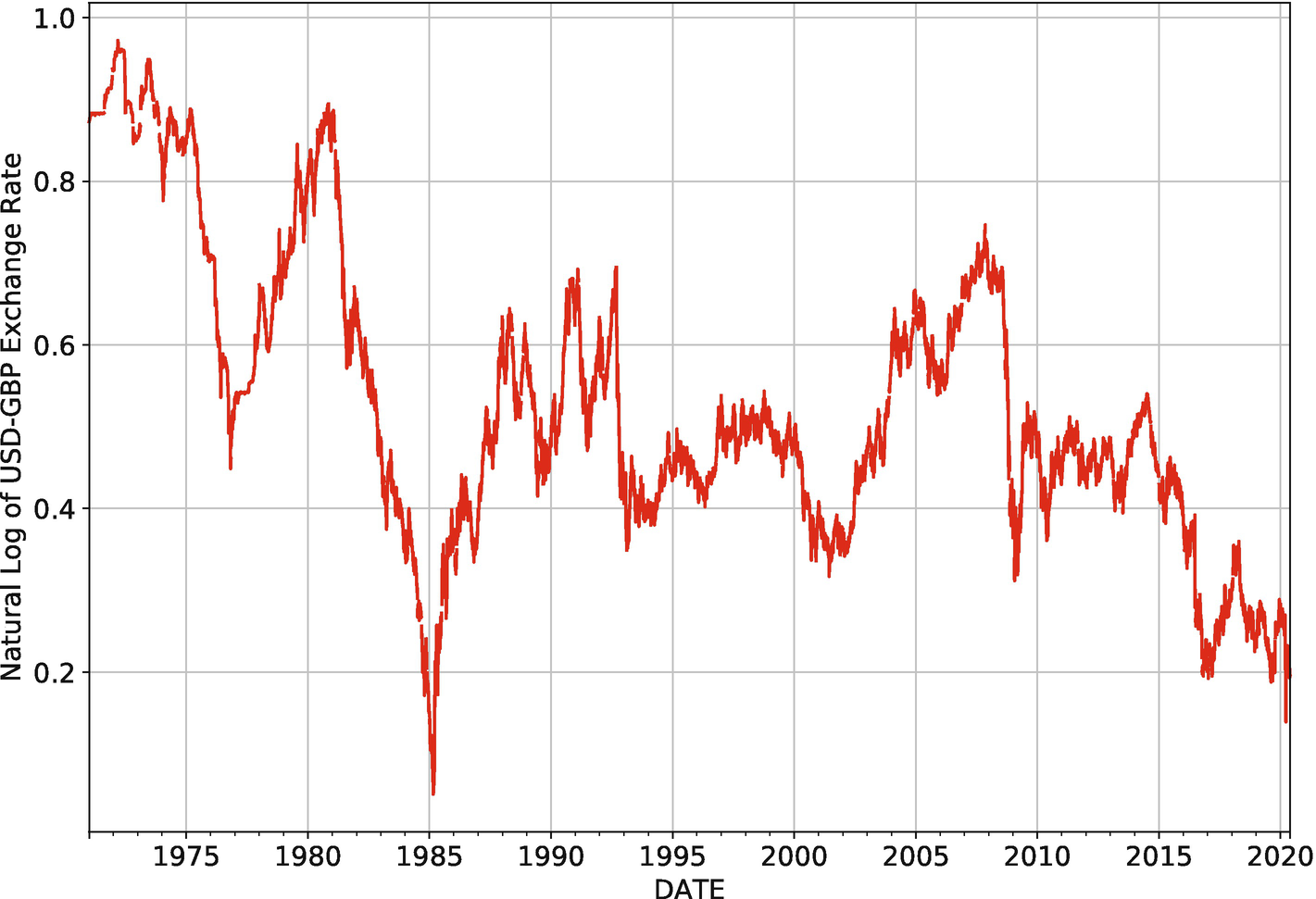
Other common loss functions for linear regression include the mean absolute percentage error (MAPE), the mean squared logarithmic error (MSLE) , and the Huber error, which are defined in Equations 3-21, 3-22, and 3-23. Respectively, these are available as tf.losses.MAPE(), tf.losses.MSLE(), and tf.losses.Huber().


Comparison of common loss functions
Optimizers
The last topic we’ll consider in this chapter is the use of optimizers in TensorFlow. We have already seen how optimizers work when we applied them in the context of linear regressions. In each case, we used the stochastic gradient descent (SGD) optimizer, which is simple and interpretable, but is less commonly used in more recent work on machine learning. In this section, we’ll expand the set of optimizers we discuss.
Stochastic Gradient Descent (SGD)
Stochastic gradient descent (SGD) is a minimization algorithm that updates parameter values through the use of the gradient. In this case, the gradient is a tensor of partial derivatives of the loss function with respect to each of the parameters.
The parameter update process is given in Equation 3-24. To ensure compatibility with the equivalent TensorFlow operation, we use the definition provided in the documentation. Note that θt is a vector of parameter values at iteration t, lr is the learning rate, and gt is the gradient computed in iteration i.

You might wonder in what sense SGD is “stochastic.” The stochasticity arises from the sampling process used to update the parameters. This differs from gradient descent, where the entire sample is used at each iteration. The benefits of the stochastic version of gradient descent are that it increases iteration speed and alleviates memory constraints.
Let’s take a look at a single SGD step for a linear regression with an intercept term and a single variable, where θt = [αt, βt]. We’ll start at iteration 0 and assume we’ve computed the gradient, g0, for the batch of data as [−0.25, 0.33]. Additionally, we’ll set the learning rate, lr, to 0.01. What does this imply for θ1? Using Equation 3-24, we can see that θ1 = [α0 + 0.025, β0 − 0.033]. That is, we decrease α0 by 0.025 and increase β0 by 0.033.
Why do we increase a parameter value when the partial derivative is negative and decrease it when it is positive? Because the partial derivatives tell us how the loss function changes in response to a change in a given parameter. If the loss function is increasing, we’re moving further away from the minimum, so we want to change direction; however, if the loss function is decreasing, we’re moving toward a minimum, so we want to continue on the same direction. Furthermore, if the loss function is neither increasing nor decreasing, this means we’re at a minimum and the algorithm will naturally terminate.

Loss function and its derivative with respect to the intercept
Returning to Equation 3-24, notice that the selection of the learning rate can also be quite consequential. If we select a high learning rate, we’ll take larger steps with each iteration, which could bring us closer to a minimum faster. However, taking larger steps could also lead us to skip over the minimum , missing it entirely. The selection of the learning rate should take this trade-off into consideration.
Finally, it is worth mentioning that the “minima” we’re identifying are local and, thus, may be higher than the global minimum. That is, SGD makes no distinction between the lowest point in an area and the lowest value of the loss function. Consequently, it may be worthwhile to re-run the algorithm for several different sets of initial parameter values to see if we always converge to the same minimum.
Modern Optimizers
While SGD is easy to understand, it is rarely used in machine learning applications in its original form. This is because modern extensions typically offer more flexibility and robustness and perform better on benchmark tasks. The most common extensions of SGD are root mean square propagation (RMSProp), adaptive moment estimation (Adam), and adaptive gradient methods (Adagrad and Adadelta).
There are several advantages to using modern extensions of SGD. First, starting with RMSProp, which is the oldest, they allow for the application of separate learning rates to each parameter. In many optimization problems, there will be orders of magnitude differences between partial derivatives in the gradient. Consequently, applying a learning rate of 0.001, for instance, may be sensible for one parameter, but not for another. RMSProp allows us to overcome this problem. It also allows for the use of “momentum,” where the gradients accumulate over mini-batches, making it possible for the algorithm to break out of local minima.
Adagrad, Adadelta, and Adam all offer variants on the use of momentum and adaptive updates for each individual parameter. Adam tends to work well for many optimization problems with its default parameters. Adagrad is centered around the accumulation of gradients and the adaptation of learning rates for individual parameters. And Adadelta modifies Adagrad by introducing a window over which accumulated gradients are retained.8
In all cases, the use of optimizers will follow a familiar two-step process. We’ll first instantiate an optimizer and will set its parameter values in the process using the tf.optimizer submodule. And second, we’ll iteratively apply the minimize function and pass the loss function to it as a lambda function.
Instantiate optimizers
For SGD, we set the learning rate and the momentum. If we’re concerned that there are many local minima, we can increase momentum to a higher value. For RMSProp, we not only set a momentum parameter but also set rho, which is the rate at which information about the gradient decays. The Adadelta parameter, which retains gradients for a period of time, also has the same decay parameter, rho. For Adagrad, we set an initial accumulator value, related to the intensity with which gradients are accumulated over time. Finally, for the Adam optimizer, we set decay rates for the accumulation of information about the mean and variance of the gradients. In this case, we have used the default values for the Adam optimizer, which generally perform well in large optimization problems.
We’ve now introduced the main optimizers we will use throughout the book. We will return to them again in detail when we apply them to train models. The modern variants of SGD will be particularly useful when we train large models with thousands of parameters.
Summary
The most commonly used empirical method in economics is the regression. In machine learning, the term regression refers to a supervised learning model with a continuous target. In economics, the term “regression” is more broadly defined and may refer to cases with binary or categorical dependent variables, such as logistic regression. For the purposes of this book, we adopt the economics terminology.
In this chapter, we introduced the concept of a regression, including the linear, partially linear, and non-linear varieties. We saw how to define and train such models in TensorFlow, which will ultimately form the basis for solving any arbitrary model in TensorFlow, as we will see in later chapters.
Finally, we discussed the finer details of the training process. We saw how to construct a loss function and what pre-defined loss functions were available in TensorFlow. We also saw how to perform minimization with a variety of different optimization routines.
Bibliography
Chernozhukov, V., D. Chetverikov, M. Demirer, E. Duflo, C. Hansen, W. Newey, and J. Robins. 2017. “Double/debiased machine learning for treatment and structural parameters.” The Econometrics Journal 21 (1).
Goodfellow, I., Y. Bengio, and A. Courville. 2017. Deep Learning. Cambridge, MA: MIT Press.
Robinson, P.M. 1988. “Root-N-Consistent Semiparametric Regression.” Econometrica 56 (4): 931–954.
Taylor, M.P., D.A. Peel, and L. Sarno. 2001. “Nonlinear Mean-Reversion in Real Exchange Rates: Toward a Solution to the Purchasing Power Parity Puzzles.” International Economic Review 42 (4): 1015–1042.