
The economics and finance disciplines have been generally reluctant to integrate forms of unstructured data. One exception to this is text, which has been applied to a wide variety of empirical problems. This may have arisen, in part, as a consequence of early successful applications in economics, such as Romer and Romer (2004), which demonstrated the empirical value of measuring internal central bank narratives.
The more widespread adoption of text may also be attributable to its many natural applications within economics and finance. It can, for instance, be used to extract latent variables, such as economic policy uncertainty from newspapers,1 consumer inflation expectations from social media content (Angelico, et al. 2018), and central bank and private firm sentiment from announcements and filings.2 It can also be used to predict bank distress (Cerchiello et al. 2017), measure the impact of news media on the business cycle (Chahrour et al. 2019), identify descriptions of fraud in consumer financial complaints (Bertsch et al. 2020), analyze financial stability (Born et al. 2013; Correa et al. 2020), forecast economic variables (Hollrah et al. 2018; Kalamara et. al 2020), and study central bank decision-making.3
The focus on textual data in economics gained renewed emphasis when Robert Shiller gave a presidential address to the American Economic Association entitled “Narrative Economics” (Shiller 2017). He argued that academic work in economics and finance has failed to account for the rise and decline of popular narratives, which have the capacity to drive macroeconomic and financial fluctuations, even if the narratives themselves are wrong. He then suggested that the discipline should begin the long project of correcting this deficiency through the exploration of text-based datasets and methods.
This chapter will discuss how text can be prepared and applied in the context of economics and finance. Throughout, we’ll use TensorFlow for modeling purposes, but will also make use of the Natural Language Toolkit (NLTK) to pre-process the data. We will also frequently refer to and use conventions from Gentzkow et al. (2019), which provides a comprehensive overview of many text analysis topics in economics and finance.
Data Cleaning and Preparation
The first step in any text analysis project is to clean and prepare the data. If, for instance, we want to use newspaper articles about a company to forecast its stock market performance, we’ll need to start by assembling a collection or “corpus” of newspaper articles and then converting the text in those articles to a numerical format.
The way in which we convert from text to numbers will determine what types of analysis we can perform. For this reason, the data cleaning and preparation step will be an important part of the pipeline for any such project. We will cover it in this subsection, focusing on its implementation using the Natural Language Toolkit (NLTK).
Install, import, and prepare NLTK
Now that we’ve installed NLTK and have downloaded all of the datasets and models, we can make use of its basic data cleaning and preparation tools. Before we can do that, though, we’ll need to prepare a dataset and introduce some notation.
Collecting the Data

The EDGAR search interface for company filings. Source: SEC.gov
Pulling up the SEC’s list of SIC codes, we can see that metal mining has been assigned the code 1000 and falls under the responsibility of the Office of Energy and Transportation, as is shown in Figure 6-2. We can now search for all filings by companies with the 1000 SIC code, yielding the results given in Figure 6-3. Each page lists companies, the state or country associated with the filing, and the Central Index Key (CIK), which can be used to identify a filing individual or corporation.

A partial list of SIC classification codes. Source: SEC.gov
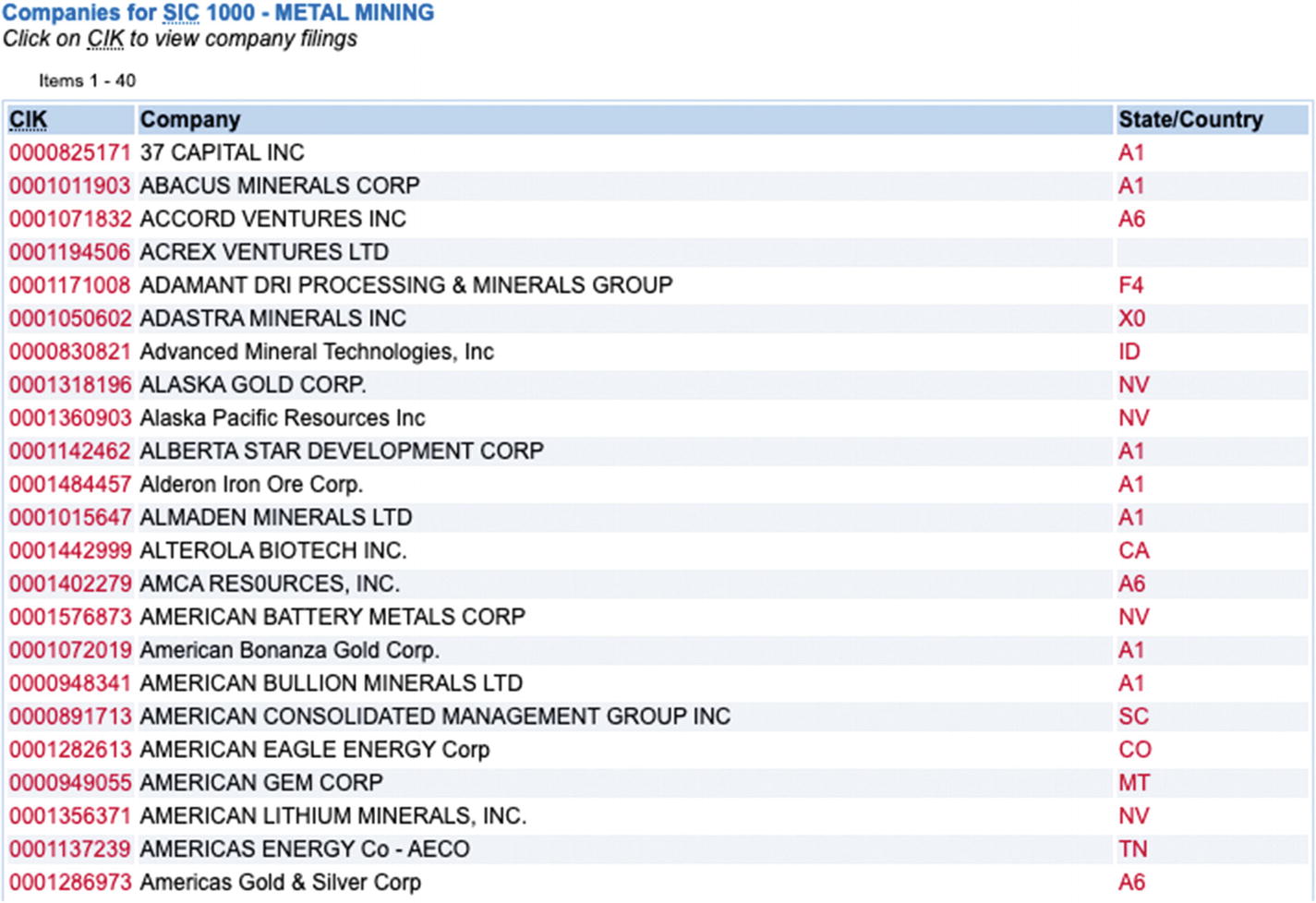
A partial list of metal mining company search results. Source: SEC.gov

A partial 6-K financial filing for a metal mining company. Source: SEC.gov
Text Data Notation
The notation we’ll use follows Gentzkow et al. (2019). We’ll let D to denote a collection of N documents or a “corpus.” C will denote a numerical array, which contains observations on K features for each document, Dj∈ D. In some cases, we’ll predict outcomes, V, using C or we’ll use fitted values,  , in a two-step casual inference problem.
- 1.
What is D?
- 2.
What features of D should be embodied in C?
If we’re working with only one 6-K filing, then Dj might be a paragraph or sentence in that filing. Alternatively, if we have many 6-K filings, then Dj is likely to represent a single filing. For the sake of fixing an example, we’ll assume that D is the collection of sentences in a single 6-K filling – namely, the one we discussed earlier.
What, then, is C? It depends on the features or “tokens” we wish to extract from each sentence of the filing. In many cases, we’ll use word counts as features; and we’ll do that in this example too. The expression for C, which is commonly referred to as the “document-feature” or “document-term” matrix is given in Equation 6-1.

Each element, cij, is the frequency with which word j appears in sentence i. A natural question we might ask is which words are included in the matrix? Should we include all words in a given dictionary? Or should we restrict it to words that appear at least once in the corpus?
Data Preparation
- 1.
Convert to lowercase : Text data is inherently high dimensional, which will force us to use dimensionality reduction strategies wherever possible. One simple way in which we can do this is to ignore capitalization. Instead of treating “gold” and “Gold” as separate features, we’ll convert all characters to lowercase and treat them as the same word.
- 2.
Remove stop words and rare words : Many words do not contain meaningful content, such as articles, conjunctions, and prepositions. For this reason, we will often compile a list of “stop words,” which will be removed from texts during the cleaning process. If our C matrix consists of word counts, knowing how many times the words “the” and “and” were used will not tell us much about our topic of interest. Similarly, when we exclude words from the document-term matrix, we will often exclude rare words, which do not appear frequently enough to allow a model to discern their meaning.
- 3.
Stem or lemmatize : The need to reduce data dimensionality further will often lead us to perform “stemming” or “lemmatization.” Stemming entails converting a word to its stem. That is, we might map the verb “running” to “run.” Since many words will map to the same stem, this will reduce the dimensionality of the problem, just as converting to lowercase letters did. Removing a word stem may result in non-word, which could be undesirable when the objective of a project is to yield interpretable outputs. In this case, we will want to consider using lemmatization instead, which maps many words to one, but uses the “base” or “dictionary” version of the word, rather than a stem.
- 4.
Remove non-word elements : In most problems we’ll encounter in economics and finance, it will not be possible to make use of punctuation, numbers, and special characters and symbols. For this reason, we will discard them, rather than including them in the document-term matrix.
Download HTML and extract text
To briefly explain the content of Listing 6-2, we first imported two submodules: urlopen from urllib.request and BeautifulSoup from bs4. The urlopen submodule allowed us to send GET requests, which is a way of requesting a file from a server. In this case, we requested the HTML document located at the specified url. We then used BeautifulSoup to create a parse tree from the HTML, so that we could make use of its structure, searching it by tag. Next, we searched for all instances of the “p” or paragraph tag. Using a list comprehension, we’ll step through each instance, returning its text attribute, which we’ll collect in a list of strings.
Join paragraphs into single string
Upon printing the corpus, we can see that it requires cleaning. It contains punctuation, stop words, line breaks, and special characters, all of which will need to be removed before computing the document-feature matrix. Now, we might be tempted to start with the cleaning step, but doing so would remove indicators of what constitutes a sentence in the text. For this reason, we’ll first split the text into sentences.
Tokenize text into sentences using NLTK
Convert characters to lowercase and remove stop words
Replace words with their stems
The last step in the cleaning process is to remove special characters, punctuation, and numbers. We’ll do this using regular expressions, which are commonly referred to as “regexes.” A regular expression is a short string that encodes a pattern that can be identified in texts. In our case, the string is [^a-z]+. The brackets indicate that the pattern is over a range of characters – namely, all the characters of the alphabet. We use the caret symbol, ^, to negate this pattern, indicating that the regex should only match characters not contained in it. This, of course, includes special symbols, punctuation, and numbers. Finally, the + symbol indicates that we allow for such symbols to be repeated in a sequence.
Remove special characters and join words into sentences
Printing the same sentence once again, we can see that it now looks quite different from its original form. Rather than a sentence, it looks like a collection of word stems. Indeed, in the following section, we will apply a form of text analysis that treats documents as a collection of words and ignores the order in which they appear. This is often referred to as the “bag-of-words” model.
The Bag-of-Words Model
In the previous section, we suggested that one possible construction of the document-term (DT) matrix, C, would use word counts as features. This representation would not allow us to account for grammar or word order, but it would permit us to capture word frequency. There are many problems in economics and finance in which we will be able to achieve our objective under such constraints.
we build a stock of utterances each of which is a particular combination of particular elements. And this stock of combinations of elements becomes a factor … for language is not merely a bag of words but a tool with particular properties which have been fashioned in the course of its use.
In this section, we’ll see how to construct a BoW model, starting with the cleaned and prepared data from the previous section. In addition to NLTK, we’ll also use submodules from sklearn to construct the DT matrix. While there are routines to perform such tasks in NLTK, they are not part of the core module and are generally less efficient.
Recall that words contained the 50 sentences we extracted from a 6-K filing for a metal mining company. We’ll use this list of lists to construct the document-term matrix in Listing 6-8, where we start by importing text from sklearn.feature_extraction . We’ll then instantiate a CounterVectorizer() , which will compute the frequency of words in each sentence and then construct the C matrix based on some constraints, which can be supplied as parameters. For the sake of illustration, we’ll set max_features to 10. This will constrain the maximum number of columns in the document-term matrix to be no higher than 10.
Construct the document-term matrix
Printing the document-term matrix and feature names, we can see that we recovered counts for ten different features. While this was useful for the sake of illustration, we will typically want to use considerably more features in actual applications; however, allowing more features may result in the inclusion of less useful features, which will necessitate the use of filtering.
Sklearn provides us with two additional parameters we can use to perform filtering: max_df and min_df. The max_df parameter determines the maximum number or proportion of documents that a term may appear in before it is removed from the term matrix. Similarly, the minimum threshold is given by min_df. In both cases, specifying an integer value, such as 3, indicates a document count, whereas specifying a float, such as 0.25, indicates a proportion of documents.
The value of specifying a maximum threshold is that it will remove all terms that appear too frequently to provide meaningful variation. If, for instance, a term appears in more than 50% of documents, we may want to remove it by specifying a max_df of 0.50. In Listing 6-9, we compute the document-term matrix again, but this time allow for up to 1000 terms and also apply filtering to remove terms that appear in either more than 50% or fewer than 5% of documents.
If we print the shape of the C matrix, we can see that it does not appear that the document-term matrix was constrained by the maximum feature limit of 1000, since only 109 feature columns were returned. This may have been a consequence of our selection of maximum document frequency and minimum document frequency parameters, which eliminated terms that were unlikely to be useful for our purposes.
Another way in which we can perform filtering is to use the term-frequency inverse-document frequency (tf-idf) metric, which is shown in Equation 6-2.
![$$ tfid{f}_j={sum}_i{c}_{ij}ast mathit{log}left(frac{N}{sum_i{1}_{left[{c}_{ij}>0
ight]}}
ight) $$](https://imgdetail.ebookreading.net/20201209/5/9781484263730/9781484263730__machine-learning-for__9781484263730__images__496662_1_En_6_Chapter__496662_1_En_6_Chapter_TeX_Equb.png)
![$$ N/{sum}_i{1}_{left[{c}_{ij}>0
ight]} $$](https://imgdetail.ebookreading.net/20201209/5/9781484263730/9781484263730__machine-learning-for__9781484263730__images__496662_1_En_6_Chapter__496662_1_En_6_Chapter_TeX_IEq2.png) . The tf-idf metric is increasing in the number of times j appears across the entire corpus and decreasing in the share of documents in which j appears. If j isn’t used frequently or is used in too many documents, the tf-idf score will be low.
. The tf-idf metric is increasing in the number of times j appears across the entire corpus and decreasing in the share of documents in which j appears. If j isn’t used frequently or is used in too many documents, the tf-idf score will be low.Adjust the parameters of CountVectorizer()
Compute inverse document frequencies for all columns
In some applications, we may want to use several words in a sequence (n-grams) – rather than individual words (unigrams) – as our features. We can do this by setting the ngram_range parameter of TfidfVectorizer() or CountVectorizer() . In Listing 6-11, we set the parameter to (2, 2), which means we only permit two-word sequences (bigrams). Note that the first value in the tuple is the minimum number of words and the second value is the maximum. We can see that the set of feature names returned is now different from the unigrams we generated in Listing 6-9.
Compute the document-term matrix for unigrams and bigrams
Dictionary-Based Methods
In the previous sections, we cleaned and prepared data and then explored it using the bag-of-words model. This yielded a NxK document-term matrix, C, which consisted of word counts for each document. We filtered certain words of the document-term matrix, but otherwise remained agnostic about what features we wished to find in the text.
An alternative to this approach is to use a pre-selected “dictionary” of words, which is constructed to capture some latent feature in the text. Such approaches are often referred to as “dictionary-based methods” and are the most commonly used form of text analysis in economics.
An early application of dictionary-based methods in economics made use of latent “sentiment” in Wall Street Journal articles to study the relationship between news and stock market performance (Tetlock 2007). Later work, such as Loughran and McDonald (2011) and Apel and Blix Grimaldi (2014), introduced dictionaries that were designed to measure specific latent variables, which lead to their widespread use in the literature. Loughran and McDonald (2011) introduced a dictionary for 10-K financial filings, which was ultimately used to measure negative and positive sentiment in many contexts. Apel and Blix Grimaldi (2014) introduced a dictionary that measured “hawkishness” and “dovishness” in central bank communication.
- 1.
The prior information you have about the latent variable and how it is represented in text is strong and reliable.
- 2.
The information about the latent variable in the text is weak and diffuse.
An ideal example of this is the Economic Policy Uncertainty (EPU) index introduced by Baker et al. (2016). The latent variable they wanted to measure was a theoretical object, which they captured in text by identifying the joint use of words that referred to the economy, policy, and uncertainty. Without specifying a dictionary for such an object, it is unlikely that it would emerge from a model as a common feature or topic. Additionally, having specified a dictionary, they demonstrated that it captured the underlying theoretical object by comparing EPU index scores with human ratings of the same newspaper articles.
Compute the Loughran-McDonald measure of positive sentiment
Next, we’ll convert the pandas Series into a DataFrame and use the column header “Positive” for the dictionary. We’ll then use a lambda function to convert all of the words to lowercase, since they are uppercase in the LM dictionary. Finally, we’ll convert the DataFrame to a list object and then print. Looking at the last three terms, we can see that two of them – winners and winning – are likely to have the same word stem.
Stem the LM dictionary
Following the steps we took earlier in the chapter, we’ll first instantiate a Porter stemmer and then apply it to each word in the dictionary using a list comprehension. The original list contains 354 words. If we then convert that list to a set, this will drop duplicate stems, reducing the number of dictionary terms to 151.
Count positive words
In Listing 6-14, we started by defining an empty list to hold the counts. We then iterated over all strings that are contained in the words list in the outer loop. Whenever we started a new sentence, we set the positive word count to 0. We then stepped through the inner loop, which iterates over all words in the stemmed LM dictionary, counting the number of times they appear in the string and adding that to the total. We appended the total for each sentence to counts.
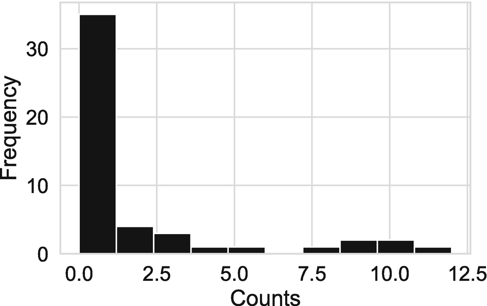
The distribution of positive word counts across sentence in a 6-K filling
In principle, we could take our positivity counts and include them as a feature in a regression. In practice, however, we will typically use a transformation of the count variable that has a more natural interpretation. If we did not have zero counts, we might use the natural logarithm of the count, allowing us to interpret the estimated effect as the impact on the percentage change in positivity. Alternatively, we could use the ratio of positive words to all words.
Finally, in economics and finance applications, it is common to use a net index, combining both positivity and negativity or “hawkishness” and “dovishness,” as is shown in Equation 6-3. Often, we will take the difference between the positive and negative word counts and then divide by a normalization factor. This factor may be the total word count for the document or the sum of the positive and negative terms.

Word Embeddings
So far, we have used one-hot encoding (dummy variables) to construct numerical representations of words. One potential downside to this approach is that we implicitly assume that each pair of words is orthogonal. The words “inflation” and “prices,” for instance, are assumed to have no relationship to each other.
An alternative to using words as features is to instead use embeddings. In contrast to word vectors, which have a high-dimensional, sparse representation, word embeddings use a low-dimensional, dense representation. This dense representation allows us to identify the degree to which words are related.
Figure 6-6 provides a simple comparison of one-hot encoded words and dense word embeddings. The statement “…inflation rose sharply…” – which might appear in a central bank announcement – could be encoded using either approach. If we use the one-hot encoded approach, shown on the left of the diagram, each word will be translated into a sparse, high-dimensional vector. And each such vector will be orthogonal to all others. If, on the other hand, if we use embeddings, each word will be associated with a lower-dimensional, dense representation, shown on the right of Figure 6-6. The relationship between two such vectors is measurable and can be captured, for instance, using their inner product. The formula for the inner product of two vectors of dimension n – x and z – is given in Equation 6-4.

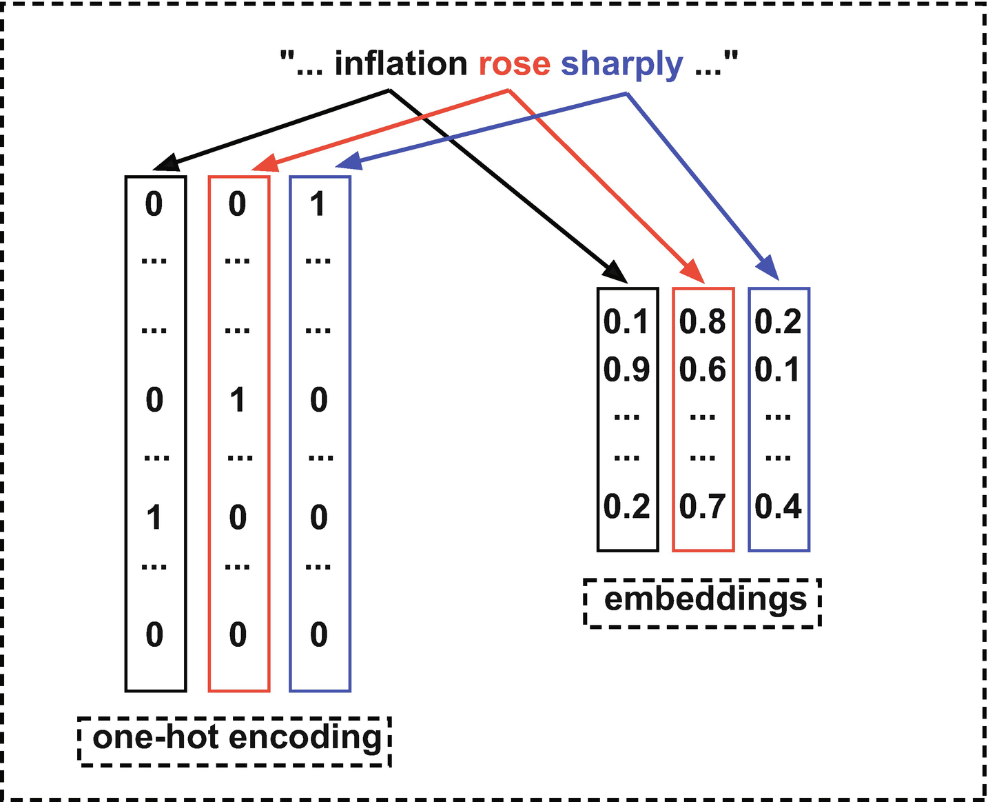
Comparison of one-hot encoding and word embeddings
While the inner product may give us a compact summary of the relationship between the two words, it does not provide more granular information about how two embedding vectors are related. For this, we can directly compare elements in the same position for a pair of vectors. Such elements provide a measurement for the same feature. While we might not be able to identify what the underlying feature is, we know that having similar values in the same position indicates two words are related along that dimension.
In contrast to one-hot encoding, we will need to use some supervised or unsupervised method to train embeddings. Since embeddings need to capture meaning in words and the relationships between words, it will often not make sense to do the training ourselves. Among other things, the embedding layer will need to learn the language in which you are performing your analysis, and the corpus you provide will almost certainly be insufficient for that task.
For this reason, you will often instead use pretrained word embeddings. Common choices include Word2Vec (Mikolov et al. 2013) and Global Vector for Word Representation (Pennington et al. 2014).
Notice that there is a strong analogy between word embeddings and convolutional layers. With convolutional layers, we said that they included general vision filters. For this reason, it often made sense to use convolutional layers from a model pretrained on millions of images. Additionally, we said that it was possible to “fine-tune” the training of such models to improve local performance on your particular image classification task. The same is also true with word embeddings.
Topic Modeling
The purpose of a topic model is to uncover a latent set of topics in a corpus and to determine the extent to which those topics are present in individual documents. The first topic model, the latent Dirichlet allocation (LDA) , was introduced to the machine learning literature in Blei et al. (2003) and has since found applications in many areas, including economics and finance.
While TensorFlow does not provide an implementation for standard workhorse topic models, it is the framework of choice for many sophisticated topic models. In general, a topic model will be more likely to be implemented in TensorFlow if it makes use of deep learning.
Since topic modeling is seeing increased use in economics, we will provide a brief introduction in this section, even though we will not make use of TensorFlow. We’ll start with a theoretical overview of the static LDA model Blei et al. (2003), followed by a description of how to implement and tune it using sklearn. We’ll will close the section by discussing recently-introduced variants of the model.
a generative probabilistic model of a corpus. The basic idea is that documents are represented as random mixtures over latent topics, where each topic is characterized by a distribution over words.
There are a few concepts worth explaining, since they will reappear throughout this chapter and text. First, the model is “generative” because it generates a novel output – the topic distribution – rather than performing a discriminative task, such as learning a classification for a document. Second, it is “probabilistic” because the model is explicitly grounded in probability theory and yields probabilities. And third, we say that topics are “latent” in that they are not explicitly measured or labeled, but are assumed to be an underlying feature of documents.
While we won’t discuss the details of solving an LDA model, we’ll briefly summarize the assumptions underlying the model in Blei et al. (2003), starting with notation. First, they assume that words are drawn from a fixed vocabulary of length V and represent them using one-hot encoded vectors. Next, they define a document as a sequence of N words, w = (w1, w2, …, wN). Finally, they define a corpus as collection of documents, D = {w1, w2, …, wM}.
- 1.
The number of words, N, in each document, w, is drawn from a Poisson distribution.
- 2.
The latent topics are drawn from a k-dimensional random variable, θ, which has a Dirichlet distribution: θ~Dir(α).
- 3.
For each word, n, a topic, zn, is drawn from a multinomial distribution that is conditional on θ. The word itself is then drawn from a multinomial distribution, conditional on the topic, zn.
The authors argue that the Poisson distribution of word counts is not an important assumption and that it would be better to use a more realistic assumption. The choice of the Dirichlet distribution constrains θ to a (k-1)-dimensional simplex. It also provides a multivariate generalization of the beta distribution and is parameterized by a k-vector of positive-valued weights, α. Blei et al. (2003) choose the Dirichlet distribution for three reasons: “…it is in the exponential family, has finite dimensional sufficient statistics, and is conjugate to the multinomial distribution.” They argued that this would ensure its suitability in estimation and inference algorithms.
The probability density of the topic distribution, θ, is given in Equation 6-5.


Plot of random draws from Dirichlet distribution with k=2 and parameter vectors [0.9, 0.1] (left) and [0.5, 0.5] (right)
We’ll next implement an LDA model, making use of the document corpus we constructed earlier by dividing a 6-K filing into sentences. Recall that we defined a document-term matrix, C, using CountVectorizer . We’ll make use of both in these in Listing 6-15, where we start by importing LatentDirichletAllocation from sklearn.decomposition. Next, we instantiate a model with our preferred parameter values. In this case, we will only set the number of topics, n_components. This corresponds to the k parameter in the theoretical model.
We can now train the model on the document-term matrix and recover the output, wordDist, using lda.components_. Note that wordDist has shape (3, 109). The rows correspond to latent topics, and the columns correspond to weights. The higher the weight, the more important a word is for defining a topic.6
We’ll next make use of the output, wordDist , to identify the words with the highest weights to for each topic. We’ll define an empty list, topics, to hold the topics. Within a list comprehension, we’ll step through each topic array and apply argsort() to recover the indices that would sort the array. We’ll then recover the last five indices and reverse their order.
For each index, we’ll identify the associated term by making use of feature_names, which we recovered from vectorizer. We’ll then print the list of topics.
Perform LDA on 6-K filing text data
Now that we have identified topics, the next step is to determine what those topics describe. In our simple example, we recovered three topics. The first appears to reference forward-looking information related to gold. The second appears to involve company operations and production. And the third topic is concerned with the cost of metals.
Assign topic probabilities to sentences
The output, as we can see in Listing 6-16, is a matrix of shape (3, 50), which contains topic probabilities that sum to one for each sentence. If, for instance, we had collected separate 6-K filings for each date, rather than looking at sentences within a filing, we’d now have the time series of topic proportions.
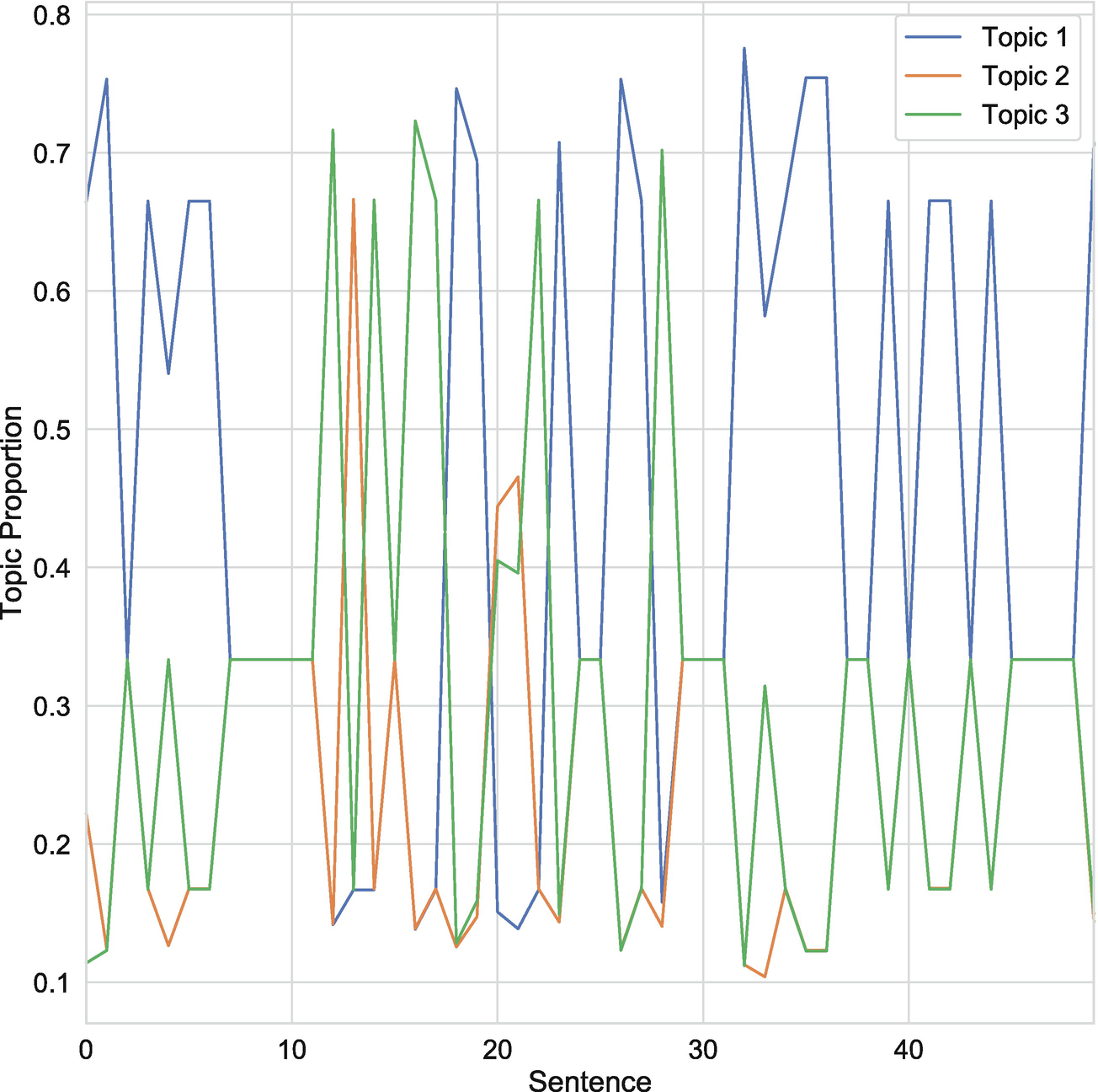
Topic proportions by sentence
- 1.
Topic prior: By default, the LDA model will use 1/n_components as the prior for all elements in α. You can, however, supply a different prior by explicitly providing a topic distribution for the parameter doc_topic_prior.
- 2.
Learning method : By default, the LDA model in sklearn will use variational Bayes to train the model and will make use of the full sample to perform each update. It is, however, possible to train in mini-batches by setting the learning_method parameter to 'online'.
- 3.
Batch size : Conditional on using online training, you will also have the option to change the mini-batch size from its default value of 128. You can do this using the batch_size parameter.
- 4.
Learning decay : When using the online learning method, the learning_decay parameter can be used to adjust the learning rate. A higher value of decay lowers the information we retain from previous iterations. The default value is 0.7, and the documentation recommends selecting a decay in the (0.5, 1] interval.
- 5.
Maximum number of iterations: Setting a maximum number of iterations will terminate the training process after that threshold has been reached. By default, the max_iter parameter is set to 128. If the model does not appear to converge within 128 iterations, you may want to set a higher value for this parameter.
Finally, two limitations of the standard LDA model introduced by Blei et al. (2003) merit discussion. First, neither the number nor content of topics may vary over the corpus. For many problems, this is not an issue; however, for applications in economics and finance that involve a time series dimension, this can be quite problematic, as we will expand on in the following paragraph. And second, the LDA model does not provide any meaningful control over the topics extracted. If we wish to track specific types of events in the data, we may not be able to do that using an LDA model, since there is no guarantee that it will identify those events.
With respect to the first problem – namely, using an LDA in time series contexts – two issues may arise. First, the model will censor topics that appear only briefly, such as financial crises, even if they are quite important during the period in which they appear. And second, it will introduce a “look-ahead” bias in the topic distribution by forcing topics that emerge in the future to also be topics in the entire sample. This can create the impression that the LDA model would have predicted events that it would not have if the sample were truncated at the date of the event.
With respect to the second problem, LDA presents two issues. The first is that we do not have the possibility to guide the model toward topics of interest. We cannot, for instance, submit topic queries to the LDA model. The second issue is that the topics the model does generate are often challenging to interpret. This is because a topic is simply a distribution over all words in the vocabulary. We will often be unable to determine what exactly a topic is without studying the distribution and examining the documents in which it is determined to be dominant.
There are, however, more recently developed models that attempt to overcome the limitations of the static LDA model. Blei and Lafferty (2006), for instance, introduce a dynamic version of the topic model. Additionally, Dieng et al. (2019) extend this further by introducing a dynamic embedded topic model (D-ETM). This model is dynamic, permits the use of a large vocabulary, and tends to generate more interpretable topics. This solves both of the issues related to the original static LDA model.
Text Regression
As Gentzkow et al. (2019) discuss, most text analysis within economics and finance centers around the bag-of-words model and dictionary-based methods. While these techniques are useful under certain circumstances, they are not the best tool for all research questions. Consequently, many projects that involve text analysis in economics could likely be improved by making use of different methods from natural language processing.
One option is to use a text regression, which is simply a regression model that includes text features, such as columns from the term-document matrix, as regressors. Gentzkow et al. (2019) argue that text regression is a good candidate method for economists to adopt. This is because economists primarily use linear regression for empirical work and often have familiarity with penalized linear regression. Thus, learning how to perform a text regression is mostly about constructing the document-term matrix, not learning how to estimate a regression.
We’ll start this section by performing a simple text regression in TensorFlow. To do this, we’ll need to construct the document-term matrix and a continuous dependent variable. Rather than using sentences within a 6-K filing, we’ll use all 8-K filings for Apple in the SEC’s system to construct the document-term matrix.7 We’ll then use the daily percentage change in Apple’s stock price on the day of the filing as the dependent variable.
For the sake of brevity, we’ll omit the details of the data collection process other than to say that we performed the same steps discussed earlier in the chapter to produce a document-term matrix, x_train, and stored the stock returns data as y_train. In total, we made use of 144 filings and extracted 25 unigram counts to construct x_train.
Recall from Chapter 3 that a linear model with k regressors has the form given in Equation 6-6. In this case, the k regressors are the feature counts from the document-term matrix. Note that we index documents using t, since we are using a time series of filings and returns.

We could, of course, make use of OLS and solve for the parameter vector with an analytical expression. However, for the sake of building toward models that are not analytically tractable, we’ll instead make use of a LAD regression. In Listing 6-17, we import tensorflow and numpy, initialize a constant term (alpha) and the vector of coefficients (beta), transform x_train and y_train into numpy arrays, and then define a function (LAD), which transforms the parameters and data into predictions.
Prepare the data and model for a LAD regression in TensorFlow
Define an MAE loss function and perform optimization
Generate predicted values from model
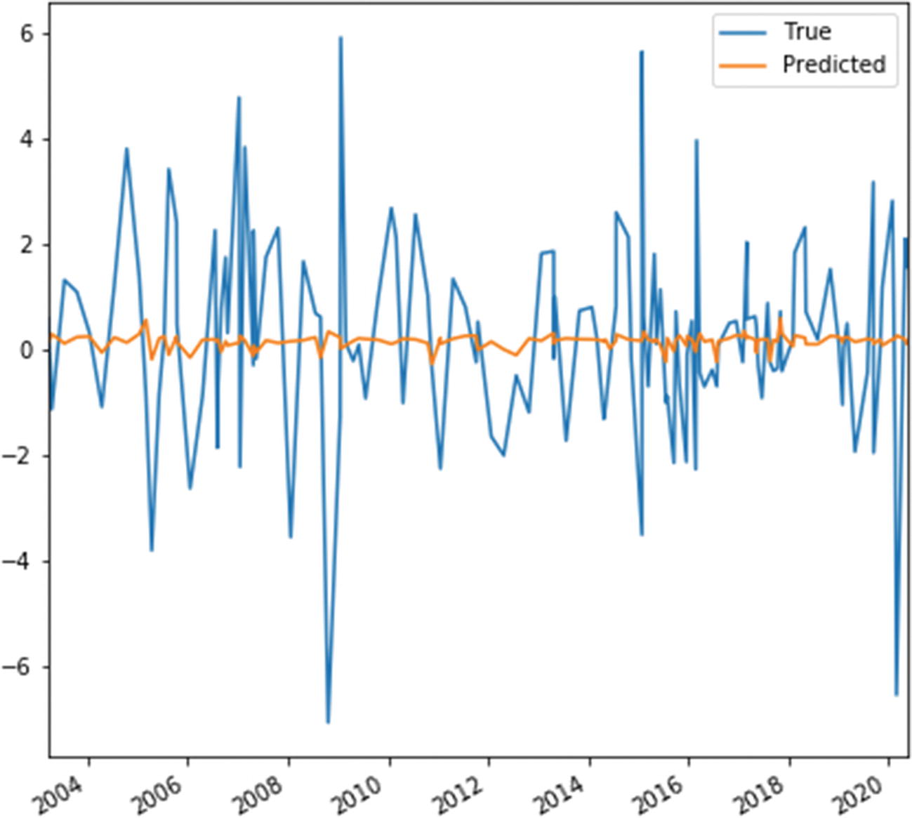
True and predicted values of Apple stock returns
There are several reasons that are unrelated to natural language processing that are likely to explain our inability to explain much of the variation in the data using the model. First, the 1-day time window could be too large and may capture developments unrelated to the announcement effect. Indeed, much of the literature in economics on the subject has moved to concentrating on narrower windows around announcements, such as 30 minutes. Second, we didn't include any non-text features in the regression, such as lagged returns, returns from the entire tech sector, or data releases from statistical agencies. And third, predicting surprise returns is challenging and even good models will typically fail to explain most of the variation in the data.
Generate predicted values from model
Many terms, as we can see in Listing 6-20, appear to be neutral. Depending on how they are modified in the text, they could predict either a positive or a negative return. If the model were able to treat the uses in their proper contexts, it might assign a large magnitude to the correctly signed feature.
We might try to fix this by expanding the set of features, performing more extensive filtering to determine the features we include, or changing the model specification to allow for non-linearities, such as feature interactions. Since we have already covered cleaning and filtering, we’ll focus on the expansion of features and the inclusion of non-linearities.
Given that the training set only contains 144 observations, we might be concerned that including more features will lead to training sample improvements, but through overfitting. This is a valid concern, and we will overcome it by using a penalized regression model. The penalty will be such that including more parameters with non-zero values will lower the value of the loss function. Thus, if the parameters do not provide considerable predictive value, we will zero them out or assign low magnitudes to them.
Gentzkow et al. (2019) define a general penalized estimator as the solution to the minimization problem in Equation 6-7.

Note that l(α, β) is a loss function, such as the MAE loss for a linear regression, λ scales the magnitude of the penalty, and κj(·) is an increasing penalty function that could, in principle, differ by parameter; however, in practice, we will often assume it is identical for all regressors.
- 1.
LASSO regression: The least absolute shrinkage and selection parameter (LASSO) model uses the L1 norm of β, reducing κ to an absolute value or ∣βj∣ for all j. The functional form of the penalty in a LASSO regression will force certain parameter values to 0, yielding a sparse parameter vector.
- 2.
Ridge regression : A ridge regression uses the L2 norm of β, yielding
 . Unlike a LASSO regression, a ridge regression will yield a dense representation of β with coefficients not set precisely to zero. Since the penalty term of a ridge regression is a convex function, it will yield a unique minimum.
 - 3.
Elastic net regression : An elastic net regression combines both the LASSO and ridge regression penalties. That is,
 for all j.
The minimization problems for LASSO, ridge, and elastic net regressions are given in Equations 6-8, 6-9, and 6-10, respectively.


We will return to the Apple stock returns prediction problem, but will now make use of a LASSO regression, which will yield a sparse coefficient vector. In our case, there were many neutral terms that likely added minimal value in a linear model, where they couldn’t be modified by adjectives. By using a LASSO regression, we’ll allow the model to decide whether to ignore them entirely by assigning a zero weight.
Before we modify the model, we’ll first apply CountVectorizer() again, but this time, we’ll construct a document-term matrix for 1000 terms, rather than 25. For the sake of brevity, we’ll omit the details and will instead start at the end of the process, where feature_names contains 1000 elements and x_train has the shape (144, 1000).
Convert a LAD regression into a LASSO regression
Train a LASSO model
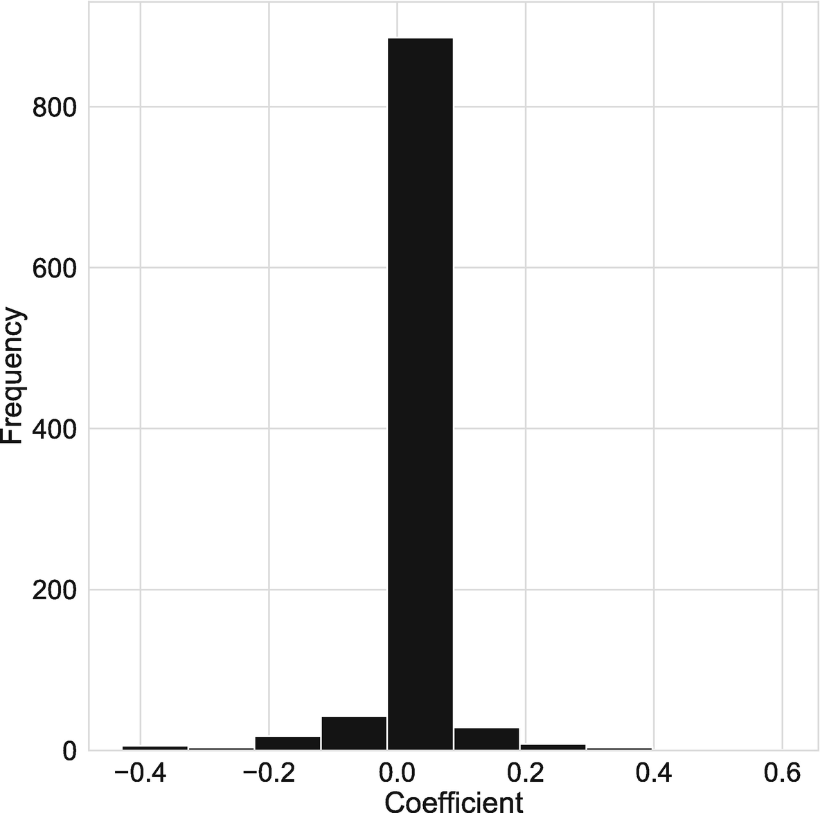
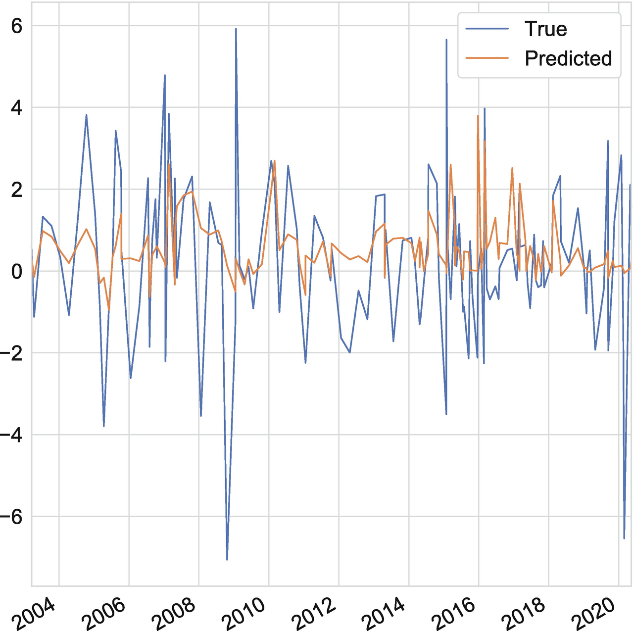
Now that we have the predicted values from the LASSO model, we can perform a comparison with the true returns. Figure 6-10 depicts this comparison, providing an update to Figure 6-9, which conducted the same exercise, but for the LAD model without a penalty term and with only 25 features.
We can see that performance has substantially improved under the LASSO model with 1000 features; however, we might worry that the penalty magnitude we selected wasn’t sufficiently severe and that the model is overfitting. To evaluate this, we can adjust lam to higher values and check the model’s performance. Furthermore, we can perform cross-validation using a test set; however, this will be somewhat more challenging in a time series context with only 144 observations.

True and predicted values of Apple stock returns using a LASSO model
True and predicted values of Apple stock returns using a LASSO model
We mentioned earlier that using a LASSO model allowed us to expand the feature set, which was one way to improve performance. Another option we mentioned was to allow for dependence between words. We can do this by permitting non-linearities in the model. In principle, we could engineer these features. We could also make use of any non-linear model to perform such a task. Furthermore, we could couple this with a penalty term, just as we did with the LASSO model, to avoid overfitting.
While these are viable strategies and can be implemented with relative ease in TensorFlow, we’ll instead make use of a more general option: deep learning. We have already discussed deep learning in the context of images in Chapter 5, but we return to it here because it provides a flexible and potent modeling strategy for most text regression problems.
The distinction between “deep learning” (e.g., neural networks) and “shallow learning” (e.g., linear regression) is that shallow learning models require us to perform feature engineering. For instance, in a linear text regression, we must decide which features are in the document-term matrix (e.g., unigrams or bigrams). We must also decide how many features to allow in the model. The model will determine which are most important for explaining variation in the data, but we must choose which to include.
Recall, again, that this was not the case with images. We input pixel values into convolutional neural networks and those networks identified successive layers of increasingly complex features. First, the networks identified edges. In the next layer, they identified corners. Each successive layer built on the previous one to identify new features that were useful for the classification task.
Deep learning can also be used in the same way for text. Rather than deciding how terms relate to each other through the use of feature engineering, we can allow a neural network to uncover these relationships for us. Just as we did in Chapter 5, we’ll make use of the high-level Keras API in TensorFlow.
In Listing 6-23, we define a neural network with dense layers that we’ll use to predict stock returns for Apple. There is only one substantive difference between this network and the dense layer-based image networks we defined in Chapter 5: the use of dropout layers. Here, we have included two such layers, each of which has a rate of 0.20. During the training phase, this will randomly drop 20% of the nodes, forcing the model to learn robust relationships, rather than using the high number of model parameters to memorize output values.8
Define a deep learning model for text using the Keras API
The architecture we’ve selected will require us to train many parameters. Recall that we can check this using the summary() method of a keras model, which we do in Listing 6-24. In total, the model has 66,177 trainable parameters.
Summarize the architecture of a Keras model
Compile and train the Keras model
As we can see in Listing 6-25, training initially reduces the loss for both the training and validation split; however, by the 15th epoch, the loss on the training split continues to decline while the loss on the validation split begins to increase slightly. This suggests that we might be starting to overfit.
True and predicted values of Apple stock returns using a neural network
If we want to reduce the risk of overfitting even further, we could increase the rates in our two dropout layers or decrease the number of nodes in the hidden layers.
Finally, note that making use of word sequences, rather than ignoring the order in which words appear, can lead to substantial improvements in model performance. This will require the use of recurrent neural networks and their variants, including the long short-term memory (LSTM) model. Since we will use the same family of models to perform time series analysis, we’ll delay their introduction to Chapter 7.
Text Classification
In the previous section, we discussed how TensorFlow could be used to perform text regression. Once we had constructed the document-term matrix, we saw that it was relatively simple to perform a LAD regression and a LASSO regression and to train a neural network. In some cases, however, we will have a discrete target and will want to perform classification instead. Fortunately, TensorFlow provides us with the flexibility to perform classification tasks by making minor adjustments to models we have already defined.
Define a logistic model to perform classification in TensorFlow
Define a loss function for the logistic model to perform classification in TensorFlow
Modify a neural network to perform classification
We changed two things: the activation function used in the outputs layer and loss function. First, we needed to use a sigmoid activation function, since we’re performing classification with two classes. And second, we used the binary_crossentropy loss, which is standard for classification problems with two classes. If we instead had a problem with multiple classes, we’d use a softmax activation function and a categorical_crossentropy loss.
For an extended overview of classification with neural networks, see Chapter 5, which covers similar material, but in the context of image classification problems. Additionally, for information about sequential models, which are commonly used for text classification problems, see Chapter 7, which makes use of the same models for time series analysis.
Summary
This chapter provided an extended overview of how text analysis is currently used in economics and finance and how it might be used in the future. The part of the process that is likely to be least familiar for economists is the data cleaning and preparation step, which transforms text into numerical data. The simplest version of this was the bag-of-words model, which stripped words from their context and summarized the content of a document using word counts alone. While this method is relatively simple to implement, it is powerful and remains one of the more commonly used methods in economics.
Dictionary-based methods also work on the bag-of-words model. However, rather than counting all terms in a document, we instead construct a dictionary that measures a latent variable. Such methods are frequently used in text analysis in economics, but are not always the best tool for many research applications, as Gentzkow et al. (2019) discuss. The EPU index (Baker, Bloom and Davis 2016) is arguably an ideal use case for dictionary-based methods in economics, since the measure is interesting for theoretical purposes, but is unlikely to emerge as a dominant topic from a corpus.
We also discussed word embeddings and saw how to implement topic models, text regression models, and text classification models. This included an overview of using deep learning models for text. We did, however, defer the discussion of sequential models to Chapter 7, which uses them for time series analysis.
Bibliography
Acosta, M. 2019. “A New Measure of Central Bank Transparency and Implications for the Effectiveness of Monetary Policy.” Working Paper.
Angelico, C., J. Marcucci, M. Miccoli, and F. Quarta. 2018. “Can We Measure Inflation Expectations Using Twitter?” Working Paper.
Apel, M., and M. Blix Grimaldi. 2014. “How Informative Are Central Bank Minutes?” Review of Economics 65 (1): 53–76.
Ardizzi, G., S. Emiliozzi, J. Marcucci, and L. Monteforte. 2020. “News and Consumer Card Payments.” Bank of Italy Economic Working Paper.
Armelius, H., C. Bertsch, I. Hull, and X. Zhang. 2020. “Spread the Word: International Spillovers from Central Bank Communication.” Journal of International Money and Finance (103).
Athey, S., and G.W. Imbens. 2019. “Machine Learning Methods that Economists Should Know About.” Annual Review of Economics 11: 685–725.
Baker, S.R., N. Bloom, and S.J. Davis. 2016. “Measuring Economic Policy Uncertainty.” Quarterly Journal of Economics 131 (4): 1593–1636.
Bertsch, C., I. Hull, Y. Qi, and X. Zhang. 2020. “Bank Misconduct and Online Lending.” Journal of Banking and Finance 116.
Blei, D.M., A.Y. Ng, and M.I. Jordan. 2003. “Latent Dirichlet Allocation.” Journal of Machine Learning Research 3: 993–1022.
Blei, D.M., and J.D. Lafferty. 2006. “Dynamic Topic Models.” ICML '06: Proceedings of the 23rd international conference on Machine Learning. 113–120.
Bloom, N., S.R. Baker, S.J. Davis, and K. Kost. 2019. “Policy News and Stock Market Volatility.” Mimeo.
Born, B., B. Ehrmann, and M. Fratzcher. 2013. “Central Bank Communication on Financial Stability.” The Economic Journal 124.
Cerchiello, P., G. Nicola, S. Ronnqvist, and P. Sarlin. 2017. “Deep Learning Bank Distress from News and Numerical Financial Data.” arXiv.
Chahrour, R., K. Nimark, and S. Pitschner. 2019. “Sectoral Media Focus and Aggregate Fluctuations.” Working Paper.
Correa, R., K. Garud, J.M. Londono, and N. Mislang. 2020. “Sentiment in Central Banks’ Financial Stability Reports.” International Finance Discussion Papers 1203, Board of Governors of the Federal Reserve System (U.S.).
Dieng, A.B., F.J.R. Ruiz, and D.M. Blei. 2019. “ The Dynamic Embedded Topic Model.” arXiv preprint.
Gentzkow, M., B. Kelly, and M. Taddy. 2019. “Text as Data.” Journal of Economic Literature 57 (3): 535–574.
Hansen, S., and M. McMahon. 2016. “Shocking Language: Understanding the Macroeconomic Effects of Central Bank Communication.” Journal of International Economics 99.
Hansen, S., M. McMahon, and A. Prat. 2018. “Transparency and Deliberation within the FOMC: A Computational Linguistics Approach.” Quarterly Journal of Economics 133: 801–870.
Harris, Z. 1954. “Distributional Structure.” Word 10 (2/3): 146–162.
Hollrah, C.A., S.A. Sharpe, and N.R. Sinha. 2018. “What’s the Story? A New Perspective on the Value of Economic Forecasts.” Finance and Economics Discussion Series 2017-107, Board of Governors of Federal Reserve System (U.S.).
Kalamara, E., A. Turrell, C. Redl, G. Kapetanios, and S. Kapadia. 2020. “Making Text Count: Economic Forecasting Using Newspaper Text.” Bank of England Staff Working Paper No. 865.
LeNail, A. 2019. “NN-SVG: Publication-Ready Neural Network Architecture Schematics.” Journal of Open Source Software 4 (33).
Loughran, T., and B. McDonald. 2011. “When is a Liability Not a Liability? Textual Analysis, Dictionaries, and 10-Ks.” Journal of Finance 66 (1): 35–65.
Mikolov, T., K. Chen, G. Corrado, and J. Dean. 2013. “Efficient Estimation of Word Representations in Vector Space.” (arXiv).
Nimark, K.P., and S. Pitschner. 2019. “News Media and Delegated Information Choice.” Journal of Economic Theory 181: 160–196.
Pennington, J., R. Socher, and C. Manning. 2014. “GloVe: Global Vectors for Word Representation.” Proceedings of the 2014 Conference on Empirical Methods in Natural Language Processing (EMNLP). Doha: Association for Computational Linguistics. 1532–1543.
Pitschner, S. 2020. “How Do Firms Set Prices? Narrative Evidence from Corporate Filings.” European Economic Review 124.
Porter, M.F. 1980. “An Algorithm for Suffix Stripping.” Program 14 (3): 130–137.
Romer, C.D., and D.H. Romer. 2004. “A New Measure of Monetary Shocks: Derivation and Implications.” American Economic Review 94: 1055–1084.
Salton, G., and M.J. and McGill. 1983. Introduction to Modern Information Retrieval. New York, NY: McGraw-Hill.
Shapiro, A.H., and D. Wilson. 2019. “Taking the Fed at its Word: A New Approach to Estimating Central Bank Objectives using Text Analysis.” Federal Reserve Bank of San Francisco Working Paper 2019-02.
Shiller, R.J. 2017. “Narrative Economics.” American Economic Review 107 (4): 967–1004.
Tetlock, P. 2007. “Giving Content to Investor Sentiment: The Role of Media in the Stock Market. ” Journal of Finance 62 (3): 1139–1168.