Relative to other machine learning packages, TensorFlow requires a substantial time investment to master. This is because it provides users with the capacity to define and solve any graph-based model, rather than providing them with a simple and interpretable set of pre-defined models. This feature of TensorFlow was intended to foster the development of deep learning models; however, it also has secondary value for economists who want to solve theoretical models.
In this chapter, we’ll provide a brief overview of TensorFlow’s capabilities in this area. We’ll start by demonstrating how to define and solve an arbitrary mathematical model in TensorFlow. We’ll then apply these tools to solve the neoclassical business cycle model with full depreciation. This model has an analytical solution, which will allow us to evaluate how well TensorFlow performed. However, we will also discuss how to evaluate performance in cases where we do not have analytical solutions.
After we demonstrate how to solve basic mathematical models in TensorFlow, we’ll end the chapter by examining deep reinforcement learning, a field that combines reinforcement learning and deep learning. In recent years, it has accumulated several impressive achievements involving the development of robots and networks that play video games with superhuman levels of performance. We’ll see how this can be applied to solve otherwise intractable theoretical models in economics.
Solving Theoretical Models
Thus far, we have defined a model by selecting a specific architecture and then training the model’s parameters using data. In economics and finance, however, we often encounter a different set of problems that are theoretical, rather than empirical, in nature. These problems require us to solve a functional equation or a system of differential equations. Such problems are derived from a theoretical model that describes optimization problems for households, firms, or social planners.
In such settings, the model’s deep parameters – which typically describe technology, constraints, and preferences – are either calibrated or estimated outside of the model and, thus, are known prior to the implementation of the solution method. The role of TensorFlow in such settings is to enable the solution of a system of differential equations.
The Cake-Eating Problem
The cake-eating problem is commonly used as a “hello world” style introduction to dynamic programming.1 In the problem, an individual is endowed with cake and must decide how much of it to eat in each period. While highly stylized, it provides a strong analogy to the standard consumption-savings problem in economics, where an individual must decide whether to consume more today or delay consumption by allocating more to savings.
As we discussed previously, the deep parameters of such models are typically calibrated or estimated outside of the solution routine. In this case, the individual consuming the cake has a utility function and a discount factor. The utility function measures the enjoyment an individual gets from consuming a piece of cake of a certain size. And the discount factor tells us how an individual will value a slice of cake today versus in the future. We will use common values of the parameters in the utility function and for the discount factor.
Formally, the cake-eating problem can be written down as a dynamic, constrained optimization problem. Equation 10-1 defines the instantaneous utility that an individual receives from eating a slice of cake at time t. In particular, we assume that the instantaneous utility received is invariant to the period in which the agent receives it: that is, we place a time subscript on c, but not u(·). We also assume that utility is given by the natural logarithm of the amount of cake consumed. This will ensure that more cake yields more utility, but the incremental gain – the marginal utility – of more cake is decreasing in c. This provides the cake-eater with a natural desire to space consumption out over time, rather than eating the entire cake today.

The marginal utility of consumption can be expressed as the derivative of u(ct) with respect to ct, as given in Equation 10-2. Notice that neither Equation 10-1 nor Equation 10-2 contains parameters. This is one of the benefits of adopting log utility for such problems: it yields simple, parameter-free expressions for utility and marginal utility and satisfies the requirements that we typically place on utility functions in economics and finance.

In addition to this, the second derivative is always negative, as can be seen in Equation 10-3.


Utility of consumption, along with its first and second derivatives over the (0,1] interval
We’ll start by considering a finite horizon problem, where the agent must divide consumption over T periods. This could be because the cake only remains edible for T periods or because the individual only lives T periods. In this stylized example, the reasoning is not particularly important, but it is, of course, more important for consumption-savings problems.
At time t = 0, the agent maximizes the objective function given in Equation 10-4, subject to the budget constraint in Equation 10-5 and a positivity constraint on st + 1 in Equation 10-6. That is, the agent must make a sequence of consumption choices, c0, …, cT − 1, each of which is constrained by the amount of remaining cake, st, and the requirement to carry a positive amount of cake, st + 1, into the following period. Additionally, consumption in all future periods is discounted by β ≤ 1.
In Equation 10-4, we also apply the Principle of Optimality (Bellman 1954) to restate the value of entering period zero with s0 cake. It will be equal to the discounted sums of utilities along the optimal consumption path, which we will denote as the unknown function, V(·).


Bellman (1954) demonstrated that we may re-express the objective function in an arbitrary period using what was later termed the “Bellman equation,” given in Equation 10-7. We also substitute the budget constraint into the equation.

Rather than choosing a consumption sequence for T-t+1 periods, we instead choose ct or the st + 1 it implies for the current period. Solving the problem then reduces to solving a functional equation to recover V(·). After doing this, choosing an st + 1 will pin down both the instantaneous utility and the discounted flows of utility from future periods, making this a sequence of one-period optimization problems.
For finite horizon problems, such as the one we’ve set up, we can pin down V(sT; T) for all sT. Since the decision problem ends in period T − 1, all choices of sT will yield V(sT; T) = 0. Thus, we’ll start by solving Equation 10-8, where it will always be optimal to consume sT − 1. We can now step back in time recursively, solving for V(·) in each period until we arrive at t = 0.

There are several ways in which we could perform the recursive optimization step. A common one is to use a discrete grid to represent the value function. For the sake of exploiting TensorFlow’s strengths and maintaining continuity with the remainder of the chapter, we’ll instead focus on a parametric approach. More specifically, we’ll parameterize the policy function that maps the state at time t, which is the amount of cake we have at the start of the period, to the state at time t+1, which is the amount of cake we carry into the following period.
To keep things simple, we’ll use a linear function for the decision rule that is proportional in the state, as shown in Equation 10-9.

We will now implement this approach in TensorFlow for the simple case where T = 2. That is, we start with a full cake of size 1 and must decide how much to carry forward to period T − 1.
Define the constants and variables for the cake-eating problem
We next define a function for the policy rule in Listing 10-2, which takes values of the parameters and yields s1. Notice that we define s1 as theta*s0. We use tf.clip_by_value() to restrict s1 to the [0.01, 0.99] interval, which imposes the positivity constraint.
Define a function for the policy rule
Define the loss function
Perform optimization
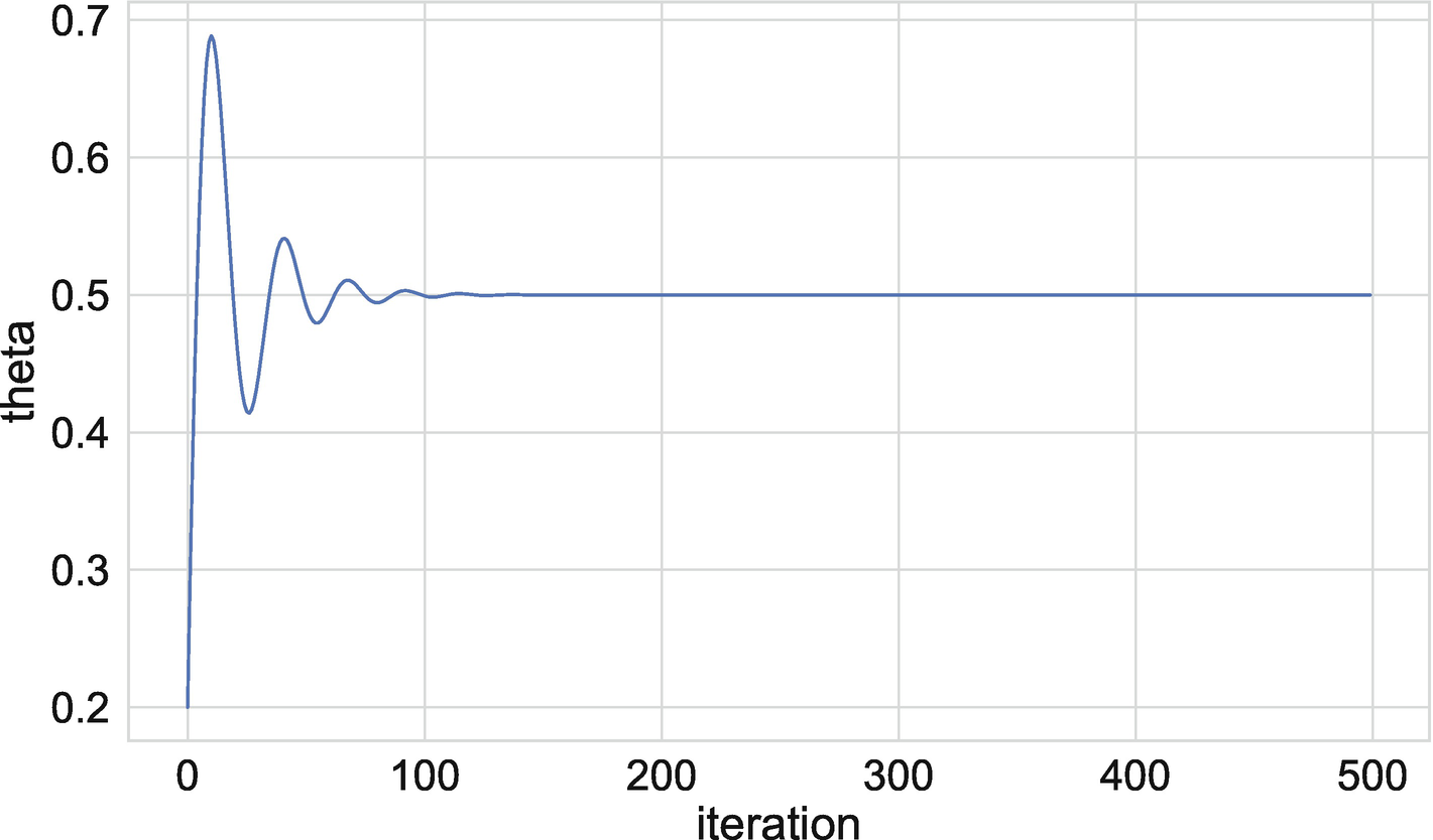
Evolution of policy function parameter over training iterations
Of course, we will typically assume a beta of less than one. Figure 10-3 plots optimal values of theta for different values of beta. In each case, we re-solve the model. As expected, we see an upward sloping relationship between the two. That is, as we place more value on the future consumption, we also choose to carry more cake forward into the future to consume.

Relationship between the discount factor and the policy rule parameter
The Neoclassical Business Cycle Model
We will end this section by solving a special form of the neoclassical business cycle model introduced by Brock and Mirman (1972). In the model, a social planner maximizes a representative household’s discounted flows of utility from consumption. In each period, t, the planner chooses next period capital, kt + 1, which yields output in the following period, yt + 1. Under the assumption of log utility and full depreciation, the model has a tractable closed-form solution.
Equation 10-10 is the planner’s problem in the initial period, which is subject to the budget constraint in Equation 10-11. The objective is similar to the cake-eating problem, but the household is infinitely lived, so we now have an infinite summation of discounted utility streams from consumption. The budget constraint indicates that the social planner divides output into consumption and capital in each period. Equation 10-12 specifies the production function.


We also assume that β < 1, α ∈ (0, 1), and capital fully depreciates in each period. This means that we recover the output produced using the capital we carried forward from the previous period, but we do not recover any of the capital itself.
One way in which we can solve this problem is by identifying a policy function that satisfies the Euler equation. The Euler equation, given in Equation 10-13, requires that the marginal utility of consumption in period t be equal to the discounted gross return to capital in period t+1, multiplied by the marginal utility of consumption in period t+1.


The Euler equation has an intuitive interpretation: a solution is optimal if the planner can’t make the household better off by reallocating a small amount of consumption from period t to period t+1 or vice versa. We will find a solution that is consistent with Equations 10-11, 10-12, and 10-13 by defining policy functions for capital and consumption. We will see, though, that the policy function for consumption is redundant.
We’ll start by assuming that the solution can be expressed as a policy function that is proportional to output. That is, the planner will choose a share of output to allocate to capital and to consumption. Equation 10-14 provides the policy function for capital, and Equation 10-15 provides the function for consumption.


The closed-form expressions for the policy functions are given in Equations 10-16 and 10-17. We will use these to evaluate the accuracy of our results in TensorFlow.


Define model parameters
Define the loss function
Perform optimization and evaluate results
Compute transition path
Finally, it is worth pointing out that we have used an intentionally trivial example where the solution can be computed analytically. In practice, we will typically encounter problems where this is not the case. In such cases, we will often use Euler equation residuals to evaluate the accuracy of the solution method.

Transition path for output, capital, and consumption
Compute the Euler equation residuals
Deep Reinforcement Learning
Standard theoretical models in economics and finance assume that agents are rational optimizers. This implies that agents form unbiased expectations about the future and achieve their objectives by performing optimization. A rational agent might incorrectly predict the return to capital in every period, but it won’t systematically overpredict or unpredict it. Similarly, an optimizer will not always achieve the best results ex-post, but ex-ante, it will have made the best decision given its information set. More explicitly, an optimizer will choose the exact optimum, given their utility function and constraints, rather than using a heuristic or rule of thumb.
As described in Palmer (2015), there are several reasons why we may wish to deviate from the rational optimizer framework. One is that we may want to focus on the process by which agents form policy rules, rather than assuming that they have adopted the one implied by rationality and optimization. Another reason is that breaking either the rationality or optimization requirement will greatly improve the computational tractability of many models.
If we do wish to depart from the standard model, one alternative approach is reinforcement learning, described in Sutton and Barto (1998). Its value within economics has been discussed in Athey and Imbens (2019) and Palmer (2015). Additionally, it was applied in Hull (2015) as a means of solving intractable dynamic programming problems.
Similar to the standard rational optimizer framework in economics, agents in reinforcement learning problems perform optimization, but they do so in an environment where they have limited information about the state of the system. This induces a trade-off between “exploration” and “exploitation” – that is, learning more about the system or optimizing over the part of the system you understand.
In this section, we’ll focus on a recently introduced variant of reinforcement learning called “deep Q-learning,” which combines deep learning and reinforcement learning. Our objective will be to slacken the computational constraints that prevent us from solving the rational optimizer versions of problems with high-dimensional state spaces, rather than studying the learning process itself. That is, we will still seek a solution for the rational optimizer’s problem, but we will do so using deep Q-learning, rather than using more conventional methods in computational economics.
Similar to dynamic programming, Q-learning is often done using a “look-up table” approach. In dynamic programming, this entails constructing a table that represents the value of being in each state. We then iteratively update that table until we achieve convergence. The table itself is the solution for the value function. In contrast, in Q-learning, we instead construct a state-action table. In our neoclassical business cycle model example, which we’ll return to here, the state was the capital stock and the action was the level of consumption.
Equation 10-18 demonstrates how the Q-table would be updated in the case where we use temporal difference learning. That is, we update the value associated with the state-action pair (st, at) in iteration i+1 by taking the value in i and adding to it to the learning rate, multiplied by the expected change in value induced by choosing the optimal action.

Deep Q-learning replaces the look-up table with a deep neural network called a “deep Q-network.” The approach was introduced in Mnih et al. (2015) and was originally applied to train Q-networks to play video games at superhuman levels of performance.
We will briefly outline how deep Q-learning can be used to solve economic models, returning to the neoclassical business cycle model example. There are several ways in which this can be done in TensorFlow. Two common options are tf-agents, which is a native TensorFlow implementation, and keras-rl2, which makes use of the high-level Keras API in TensorFlow. Since our coverage will be brief and introductory, we’ll focus on keras-rl2, which will allow for a simpler implementation with more familiar syntax.
Install and import modules to perform deep Q-learning
In Listing 10-11, we’ll set the number of capital nodes and define an environment, planner, which is a subclass of gym.Env. This will specify the details of the social planner’s reinforcement learning problem.
Define custom reinforcement learning environment
We next define a step method of the class, which is required to return four outputs: the observation (state), the reward (instantaneous utility), an indicator for whether a training session should be reset (done), and a dictionary object that contains relevant debugging information. Calling this method increments the decision_count attribute, which records the number of decisions an agent has made during a training session. It also initially sets done to False. We then evaluate whether the agent made a valid decision – that is, selected a positive value of consumption. If an agent makes more than decision_max decisions or chooses a non-positive consumption value, the reset() method is called, which reinitializes the state and decision count.
Instantiate environment and define model in TensorFlow
Set model hyperparameters and train
Monitoring the training process yields two observations. First, the number of decisions per session increases across iteration, suggesting that the agent learns to avoid negative amounts of future periods by not drawing capital down as sharply as a greedy policy might suggest. And second, the loss declines and the average reward begins to rise, suggesting that the agent is moving closer to optimality.
If we wanted to perform a more thorough analysis of the quality of our solution, we could examine the Euler equation residuals, as we discussed in the previous section. This would tell us whether the DQM model yielded something that was approximately optimal.
Summary
TensorFlow not only provides us with a means of training deep learning models but also offers a suite of tools that can be used to solve arbitrary mathematical models. This includes models that are commonly used in economics and finance. In this chapter, we examined how to do this using a toy model (the cake-eating model) and a common benchmark in the computational literature: the neoclassical business cycle model. Both models are trivial to solve using conventional methods in economics, but provide a simple means of demonstrating how TensorFlow can be used to solve theoretical models of relevance for economists.
We also showed how deep reinforcement learning could be used as an alternative to standard methods in computational economics. In particular, using deep Q-learning networks (DQN) in TensorFlow may enable economists to solve higher-dimensional models in a non-linear setting without changing model assumptions or introducing a substantial amount of numerical error.
Bibliography
Athey, S., and G.W. Imbens. 2019. “Machine Learning Methods Economist Should Know About.” Annual Review of Economics 11: 685–725.
Bellman, R. 1954. “The theory of dynamic programming.” Bulletin of the American Mathematical Society 60: 503–515.
Brock, W., and L. Mirman. 1972. “Optimal Economic Growth and Uncertainty: The Discounted Case.” Journal of Economic Theory 4 (3): 479–513.
Hull, I. 2015. “Approximate Dynamic Programming with Post-Decision States as a Solution Method for Dynamic Economic Models.” Journal of Economic Dynamics and Control 55: 57–70.
Mnih, V. et al. 2015. “Human-level control through deep reinforcement learning.” Nature 518: 529–533.
Palmer, N.M. 2015. Individual and Social Learning: An Implementation of Bounded Rationality from First Principles. Doctoral Dissertation in Computational Social Science, Fairfax, VA: George Mason University.
Sutton, R.S., and A.G. Barto. 1998. Reinforcement Learning: An Introduction. Cambridge: MIT Press.