Empirical work in economics is typically concerned with causal inference and hypothesis testing, whereas machine learning is centered around prediction. There is, however, a clear intersection between objectives when it comes to forecasting in economics and finance. Consequently, there has been increasing interest in using methods from machine learning to produce and evaluate economic forecasts.
In Chapter 2, we discussed Coulombe et al. (2019), which evaluated the usefulness of machine learning for time series econometrics. They identified non-linear models, regularization, cross-validation, and alternative loss functions as potentially valuable tools that could be imported for use in time series econometric contexts.
In this chapter, we’ll discuss the value of machine learning for time series forecasting. Since we’ll concentrate on a TensorFlow implementation, our focus will diverge from Coulombe et al. (2019) and instead concentrate on deep learning models. In particular, we will make use of neural network models with specialized layers that are used to process sequential data.
Throughout the chapter, we’ll build on a forecasting exercise (Nakamura 2005), which was one of the first applications of neural networks in time series econometrics. Nakamura (2005) used a dense neural network to demonstrate gains over a univariate autoregressive model for forecasting inflation.
Sequential Models of Machine Learning
Thus far, we have discussed several specialized layers for neural networks, but have not explained how to handle sequential data. As we will see, there are robust frameworks for handling such data in neural networks, which were largely developed for the purpose of natural language processing (NLP), but are equally useful in time series contexts. We will also briefly return to their use in NLP contexts at the end of the chapter.
Dense Neural Networks
We have already used dense neural networks in Chapters 5 and 6; however, we have not explained how they can be adapted for use with sequential data. So far, all of our uses of neural networks involved exercises that lacked or did not exploit a time dimension.
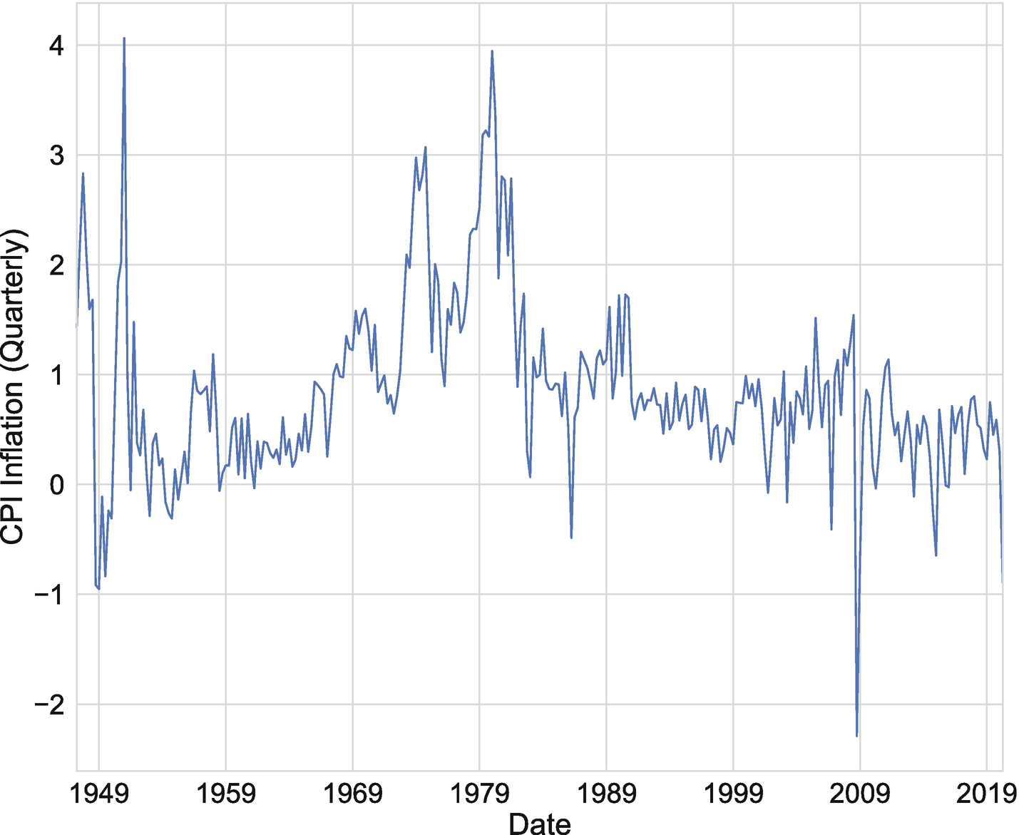
We’ll start this section by examining how to make use of sequence data to predict quarterly inflation in a setting similar to Nakamura (2005). To conduct this exercise, we’ll use quarterly inflation for the United States over the period between 1947:Q2 and 2020:Q2,1 which is plotted in Figure 7-1. Additionally, following Nakamura (2005), we’ll consider univariate models, where we do not include any additional explanatory variables beyond lags of inflation.
When we worked with text and image data in earlier chapters, we often needed to perform pre-processing tasks to transform the raw inputs into something suitable for use in a neural network. With sequential data, we will also need to transform the time series into sequences of fixed length.
Figure 7-1
CPI inflation over the period between 1947:Q2 and 2020:Q2. Source: US Bureau of Labor Statistics
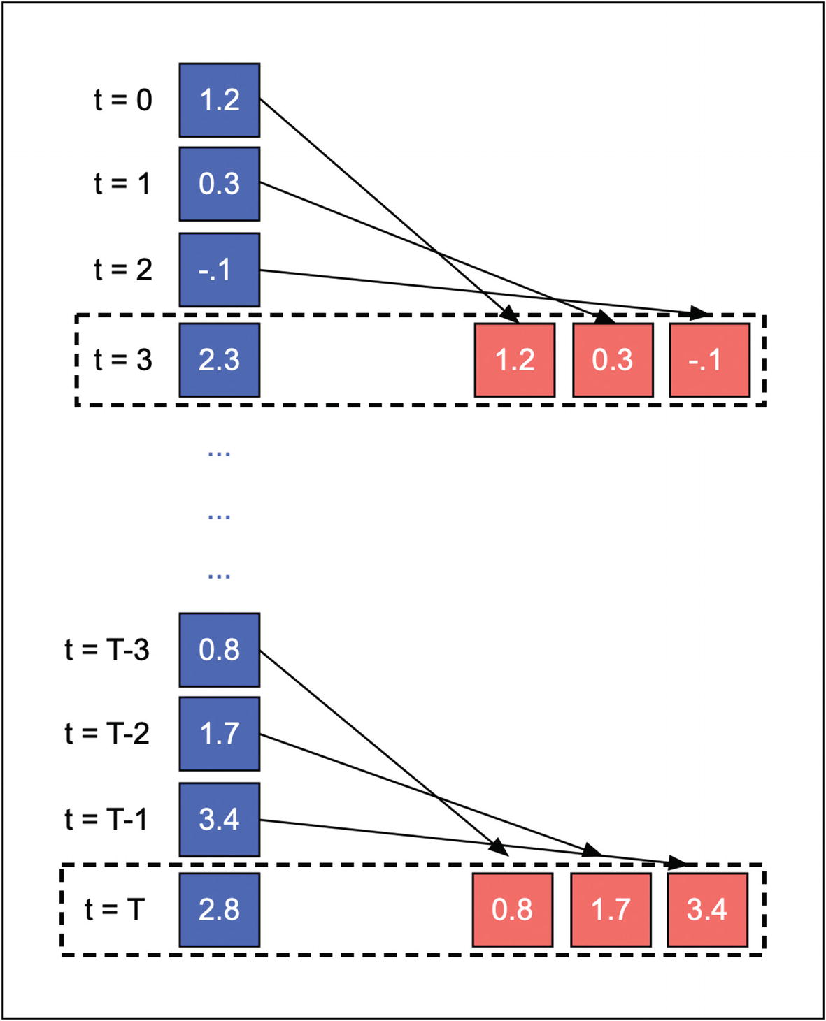
We’ll start by deciding the sequence length, which is the number of lags we’ll use as inputs to the neural network. If, for instance, we select a sequence length of three, then the network will predict inflation in period t+h using the realizations in periods t, t-1, and t-3. Figure 7-2 illustrates the pre-processing step, where we split a single time series into overlapping sequences of three consecutive observations. The left side of the diagram shows the original input series. The right side shows two examples of sequences. The dashed rectangles connect the sequences with the value they would predict if we use a single quarter as the forecast horizon (h=1).
Figure 7-2
Division of time series into overlapping sequences of three consecutive observations
We’ll assume the data has been downloaded and saved as inflation.csv in a directory located at data_path. We’ll start by loading it with pandas in Listing 7-1 and then converting it into a numpy array. Next, we’ll define a generator object using TimeseriesGenerator() from the tensorflow.keras.preprocessing.sequence submodule. As inputs, it will take the network’s features and target, the length of the sequence, and the batch size. In this case, we’ll perform a univariate regression, where the feature and target are both inflation. We’ll use a sequence length of 4, which we can set using the length parameter. Finally, we’ll use a batch_size of 12, which means that our generator will yield 12 sequences and 12 target values each iteration.
import numpy as np
import tensorflow as tf
from tensorflow.keras.preprocessing.sequence import TimeseriesGenerator
We now have a generator object that we can use to create batches of data. A Keras model can use the generator, rather than data, as an input. In Listing 7-2, we’ll define a model and then train it using the generator. Note that we use a Sequential() model. This enables us to construct a model by stacking layers in sequence and does not have anything to do with the use of sequential data.
We first instantiate the model using the sequential API. We then set the number of input nodes to match the sequence length, define a single hidden layer with two nodes, and define an output layer that uses a linear activation function, since we have a continuous target. Finally, we’ll compile the model using the mean squared error loss and an adam optimizer.
When we trained models previously, we used np.array() or tf.constant() objects as input data. In Listing 7-2, we’ve used a generator, which will require us to use the fit_generator() method, rather than fit(), as we have previously.
Between epochs 1 and 100, the model makes considerable progress in reducing mean squared error, lowering it from 4.32 to 0.38. Importantly, we have not used regularization, such as dropout, and have not created a test sample split, so it is possible that there is substantial overfitting. In Listing 7-3, we use the summary() method of model to examine its architecture. We can see that it has only 13 trainable parameters, which is small in comparison to the models we have worked with previously.
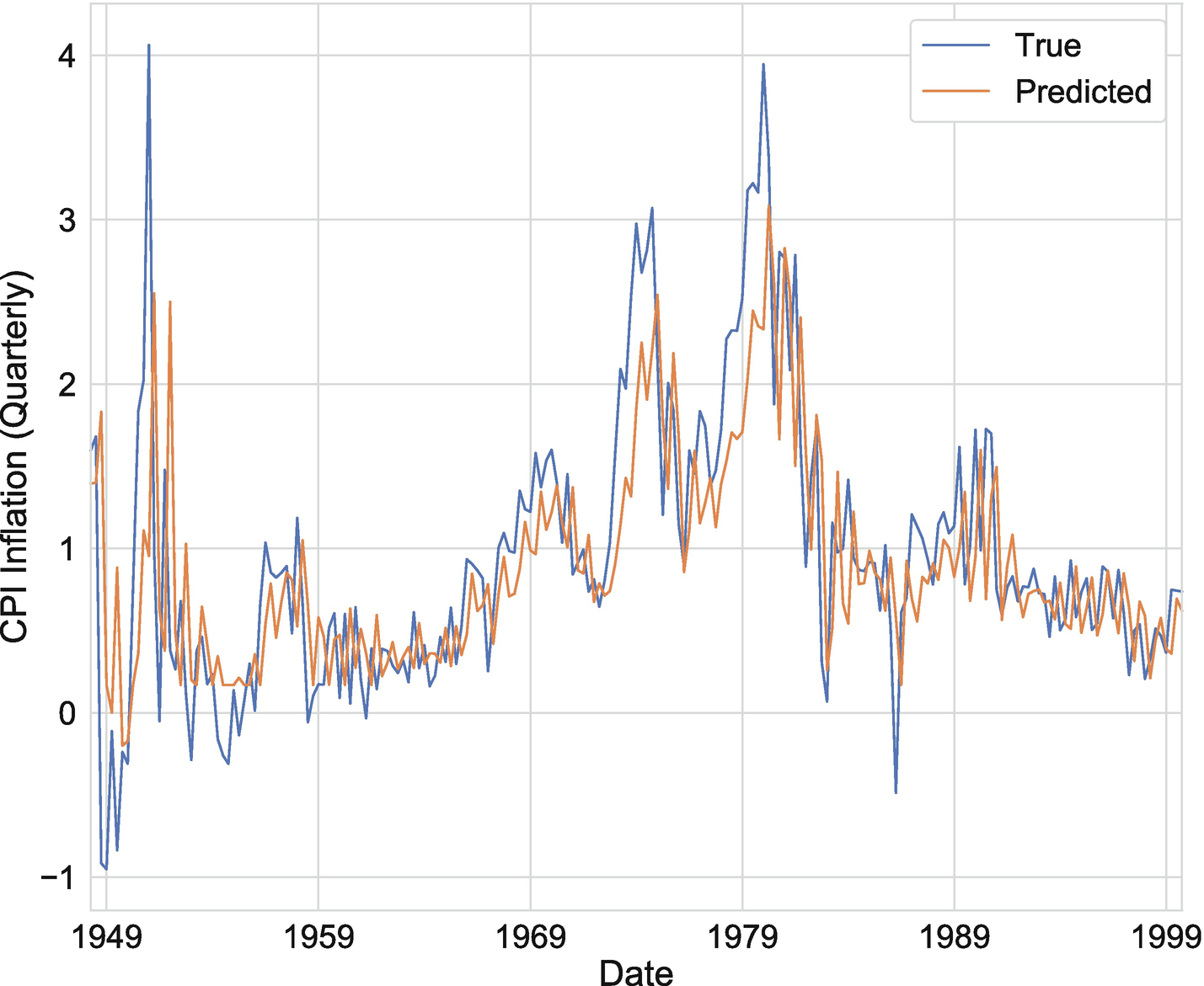
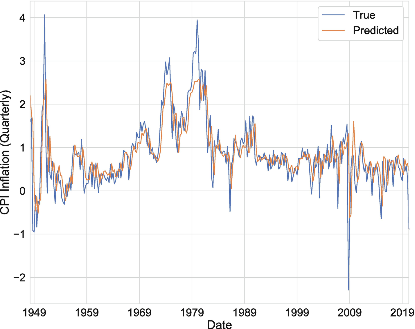
We can now use model.predict_generator(generator) to generate a series of predicted values for inflation. Figure 7-3 plots the true values of inflation against our model’s prediction. While model performance looks compelling, we have not yet taken the proper precautions to ensure that we are not overfitting.
In Figure 7-4, we examine whether overfitting is an issue for this by using the post-2000 period as the test sample. To do this, we need to construct a separate generator, which only uses the pre-2000 values to train. We then use our original generator to make predictions for the entire sample, including the post-2000 values.
Figure 7-3
Dense network one-quarter-ahead forecast of inflation
We can see that Figure 7-4 does not look substantially different from Figure 7-3 post 2000. In particular, there does not appear to be a performance degradation after 2000, which is what we would expect if the model were overfitting on the pre-2000 data. This is not too surprising, since the model has relatively few parameters, making it more difficult to overfit.
In the remainder of this section, we will make use of the same pre-processing steps, but will add specialized layers to our model that are designed to handle input sequences. These layers will exploit the temporal information encoded in the lag structure, rather than treating all features the same, as we are currently doing with the dense model.
Figure 7-4
Dense network one-quarter-ahead forecast of inflation in model trained on data from 1947 to 2000
Recurrent Neural Networks
A recurrent neural network accepts a sequence of inputs and processes them using a combination of dense layers and specialized recurrent layers (Rumelhart et al. 1986).2 This sequence of inputs could be word vectors, word embeddings, musical notes, or, as we will consider in this chapter, inflation measurements at different points in time.
We will follow the treatment of recurrent neural networks (RNNs) given in Goodfellow et al. (2017). The authors describe a recurrent layer as consisting of cells that each take an input value, x(t), and a state, h(t − 1), and produce an output value, o(t). The process by which the output value is produced for a recurrent cell is given by Equations 7-1, 7-2, and 7-3.
In Equation 7-1, we take the state of the series, h(t − 1), and multiply it by weights, W. We then take the input value, x(t), and multiply it by a separate set of weights, U. Finally, we sum both terms together, along with a bias term, b.
Equation 7-1. Performing themultiplication stepfor an RNN cell.
We next take the output of the multiplication step and pass it to a hyperbolic tangent activation function, as shown in Equation 7-2. The output of this step is the updated state of the system, h(t).
Equation 7-2. Applying an activation function in an RNN cell.
In the final step, given in Equation 7-3, we multiply the updated state by a separate set of weights, V, and add a bias term.
Equation 7-3. Generating theoutput valuefrom an RNN cell.
In the example we’re working with in this chapter, inflation is the only feature. This means that x(t) is a scalar and W, U, and V are also scalars. Additionally, notice that these weights are shared for all time periods, which reduces the model size relative to what would be needed with a dense network. In our case, we will only need five parameters for a layer with one RNN cell.
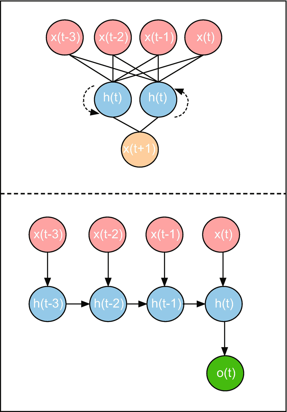
Figure 7-5 provides a complete illustration of an RNN. The pink nodes indicate input values, which are lags of inflation in our example. The orange node indicates the target variable, which is inflation in the following quarter. The blue nodes are individual RNN cells, which form an RNN layer. The network we’ve illustrated has four inputs and two RNN cells.
Figure 7-5
Illustration of a RNN (top) and unrolled RNN cell (bottom)
The bottom panel of Figure 7-5 shows an “unrolled” RNN cell, where the cell’s iterative structure has been broken down into a sequence. In each individual step, the state is combined with an input to yield the next state. The final step yields an output, o(t), which is an input to a final dense layer – along with the outputs of the other cells – that yields a prediction for inflation one quarter ahead.
We’ve now seen that an RNN makes use of sequential data by retaining a state, which it updates at each step of the sequence. It also reduces the number of parameters through the use of weight sharing. Furthermore, since it is not necessary to apply time-specific weights, it will also be possible to use RNN cells with sequences of arbitrary and variable length.
We have now discussed how an RNN differs from a dense network. Let’s construct a simple RNN for our inflation forecasting example. We’ll start by loading the data in Listing 7-4. Here, we’ve repeated the steps from Listing 7-1, but with two important differences. First, we use np.expand_dims() to add a dimension to the inflation array. This will allow our time series data to conform to the input shape requirements of RNN cells in Keras. And second, we’ve defined a train generator, which exclusively uses data prior to 2000 by slicing the inflation array, retaining only the first 211 observations.
Once we have loaded and prepared our data, the next step is to define the model, which we do in Listing 7-5. As we can see, the model requires no more lines of code than did the dense network we used to predict inflation. All we do is define a sequential model, add an RNN layer, and define a dense output layer with a linear activation function.
Notice that the SimpleRNN layer we used required two arguments: the number of RNN cells and the shape of the input layer. For the first argument, we selected two cells to keep the network simple at the potential risk of underfitting the data. We needed to provide the second argument because we defined the RNN layer as the first in our network. We set the input_shape to be (4, 1) because the sequence length is four and the number of features is one.
import numpy as np
import tensorflow as tf
from tensorflow.keras.preprocessing.sequence import TimeseriesGenerator
The final steps are to compile the model and to use the fit_generator() method to train it, along with the train_generator we constructed earlier. As we can see in Listing 7-6, the model achieves a lower mean squared error (0.2594) than we were able to achieve in the dense network with 100 epochs of training. Additionally, as shown in Figure 7-6, test sample performance (post-2000) does not appear to degrade in any noticeable way.
We also mentioned that the RNN model has the benefit of requiring fewer parameter values than a dense network. When we stepped through the operations performed in an RNN cell, we saw that only five parameters were needed for a layer with a single RNN cell. In Listing 7-7, we’ll use the summary() method of model to explore the model’s architecture. We can see that it has eight parameters in the RNN layer and three in the dense output layer. In total, it has 11 parameters, which is fewer than the dense network we used earlier. The contrast is not particularly large here, of course, since both networks are quite small.
Figure 7-6
One-quarter-ahead forecast of inflation for RNN model trained on data from 1947 to 2000
In practice, we will not typically use an RNN model without modification. At a minimum, there are at least two things we will want to consider adjusting. The first is related to a technical problem – the “vanishing gradient problem” – which makes it challenging to train deep networks. This is also a problem with the original RNN model and long sequences of data. Another problem with the original RNN model is that it does not allow for the possibility that objects far apart in time or within the sequence are more closely related than objects nearer together. In the following two subsections, we’ll make some minor adjustments to the RNN model that will allow us to deal with both problems.
Long Short-Term Memory (LSTM)
The first problem with RNNs is that they suffer from the vanishing gradient problem when long sequences of data are used as inputs. The most effective solution to this problem is to make use of a gated RNN cell. There are two such cells that are commonly used: (1) long short-term memory (LSTM) and (2) gated recurrent units (GRUs). We will concentrate on the former in this subsection.
The LSTM model was introduced by Hochreiter and Schmidhuber (1997) and functions through the use of operators that limit the follow of information in long sequences. We will again follow Goodfellow et al. (2017) in describing the operations performed in an LSTM.
Equations 7-4, 7-5, and 7-6 define the “forget gate,” “external input gate,” and “output gate,” all of which play a role in controlling the follow of information through an LSTM cell.
Equation 7-4. Definition of trainable weights called forget gates.
Equation 7-5. Definition of trainable weights called external input gates.
Equation 7-6. Definition of trainable weights called output gates.
Notice that each gate has the same functional form and uses a sigmoid activation function, but has its own separate weights and biases. This allows the gating procedure to be learned, rather than applied from a fixed rule.
The internal states are updated using the expression in Equation 7-7, where the forget gate, external input gate, input sequence, and state are all applied.
Equation 7-7. Expression for updating the internal state.
Finally, we update the hidden state, making use of the internal state and the output gate, as in Equation 7-8.
Equation 7-8. Expression for updating the hidden state.
While the use of gates increases the number of parameters in the model, it also yields substantial improvements in the handling of long sequences in many practical applications. For this reason, we will typically use an LSTM model as the baseline in time series analysis, rather than the original RNN model.
In Listing 7-8, we define and train an LSTM model using 100 epochs. The only difference was that we used tf.keras.layers.LSTM(), rather than tf.keras.layers.SimpleRNN(). We can see that mean squared error is higher for the LSTM than it was for the RNN after 100 epochs. This is because the model must train more weights, which will require additional training epochs. Additionally, the LSTM is likely to be most useful in settings with longer sequences.
Finally, in Listing 7-9, we summarize the model’s architecture. When we discussed the additional operations an LSTM cell required, we mentioned that it introduced a forget gate, an external input gate, and an output gate. All of these required their own set of parameters. As we can see from Listing 7-9, the LSTM layer uses 32 parameters, which is four times as many as the RNN.
By convention, the LSTM model only makes use of the final value of the hidden state. In Figure 7-5, for instance, the model uses h(t) and not h(t − 1), h(t − 2), and h(t − 3), even though we computed them. Recent work, however, has shown that using the intermediate hidden states can lead to considerable improvements in modeling long-term dependencies, especially in natural language processing problems (Zhou et al. 2016). This is typically done in the context of an attention model.
We will not discuss the attention model here, but will explain how to make use of hidden states in an LSTM model. Let’s start by naively setting the LSTM cells in our model from Listing 7-8 to return hidden states by setting return_sequences to True. We’ll do that in Listing 7-10 and then check the model’s architecture using the summary() method.
As we can see, there’s something unusual about the model’s architecture: rather than outputting a scalar prediction for each observation in the batch, it instead outputs a 4x1 vector. This appears to be a consequence of the LSTM layer, which is now outputting 4x1 vectors, rather than scalars, from each of its two LSTM cells.
There are several ways in which we can make use of the LSTM output. One such method is called a stacked LSTM (Graves et al. 2013). This works by passing the full sequence hidden states to a second LSTM layer, creating depth in the network that allows for more than one level of representation.
In Listing 7-11, we define such a model. In the first LSTM layer, we use a layer with three LSTM cells and an input shape of (4, 1). We set return_sequences to True, which means that each cell will return a 4x1 sequence of hidden states, rather than a scalar. We’ll then pass this 3-tensor (4x1x3) to a second LSTM layer with two cells, which only returns the final hidden states and not intermediate state values.
The model’s architecture is summarized in Listing 7-12. We can see that it now outputs a scalar prediction, which is what we want for the inflation forecast. We will omit an analysis of model performance, but will point out that the use of such models for time series forecasting remains underexplored. It is possible that using stacked LSTM models, the attention model, or the transformer model could lead to improvements in time series forecasting in cases where modeling long-run dependencies is important.
So far, we have focused on the mechanics of different methods and have structured all examples around the univariate inflation forecasting exercise in Nakamura (2005). The methods we have discussed all carry over to a multivariate setting. For the sake of completeness, we will provide a brief multivariate forecasting example, making use of both the LSTM model and gradient boosted trees, which we discussed in Chapter 4. We will, again, attempt to forecast inflation, but will do so at a monthly frequency and using five features, rather than one.
We’ll start by loading and previewing the data in Listing 7-13. We’ll then discuss how to implement a multivariate forecast model using an LSTM and gradient boosted trees. The four features we’ve added are unemployment, hours worked in the manufacturing sector, hourly earnings in the manufacturing sector, and a measure of the money supply (M1). Unemployment is measured in first differences, whereas all level variables transformed using percentage changes from the previous period.
As we saw earlier in the chapter, we can prepare the data for use in an LSTM model by instantiating a generator. We’ll first convert the target and features to np.array() objects. We’ll then create one generator for training data and another for test data. In the previous example, we used quarterly data and four-quarter sequence lengths. In this case, we’ll use monthly data and 12-month sequence lengths in Listing 7-14.
import numpy as np
import tensorflow as tf
from tensorflow.keras.preprocessing.sequence import TimeseriesGenerator
With the generators defined, we can now train the model in Listing 7-15. We’ll use two LSTM cells. Additionally, we’ll need to change the input shape, since we now have 12 elements in each sequence and five features. Over 20 epochs of training, the model reduces the mean squared error from 0.3065 to 0.0663. If you’ve done macroeconomic forecasting using econometric models, you might worry about the number of model parameters, since we’re using longer sequences and more variables; however, for the reasons we discussed earlier, the longer sequence length does not increase the number of parameters. In fact, the model has only 67 parameters.
Define and train LSTM model with multiple features
Finally, in Listing 7-16, we’ll evaluate the model by comparing the training sample results to the test sample results. We can see that the training set performance appears to be better than test set performance, which is common; however, if the disparity becomes sufficiently large, we should consider using regularization or terminating the training process after fewer epochs.
# Evaluate training set using MSE.
model.evaluate_generator(train_generator)
0.06527029448989197
# Evaluate test set using MSE.
model.evaluate_generator(test_generator)
0.15478561431742632
Listing 7-16
Use MSE to evaluate train and test sets
Gradient Boosted Trees
As a final example, we’ll consider performing the same forecasting exercise, but using gradient boosted trees, which we discussed in Chapter 4. Within the set of tools TensorFlow offers, gradient boosted trees and deep learning are most suitable for time series forecasting tasks.
Just as LSTM models require us to prepare data by splitting it into sequences, gradient boosting with trees will require us to prepare the data in a format usable in the Estimator API. This will involve defining feature columns for each of the five features, as we do in Listing 7-17.
The next step is to define functions that generate data. We’ll do this separately for train and test functions, so that we can evaluate overfitting, just as we did for the LSTM example. Listing 7-18 defines the two functions. Again, we use the same sample split: the train set will cover the years prior to 2000, and the test set will cover the years afterward.
# Define lagged inflation feature column.
inflation = tf.feature_column.numeric_column(
"inflation")
# Define unemployment feature column.
unemployment = tf.feature_column.numeric_column(
"unemployment")
# Define hours feature column.
hours = tf.feature_column.numeric_column(
"hours")
# Define earnings feature column.
earnings = tf.feature_column.numeric_column(
"earnings")
# Define M1 feature column.
m1 = tf.feature_column.numeric_column("m1")
# Define feature list.
feature_list = [inflation, unemployment, hours,
earnings, m1]
Listing 7-17
Define feature columns
In Listing 7-19, we train a BoostedTreeRegressor using 100 epochs and train_data. We then perform evaluation on both the training and test sets and print the results.
# Define input function for training data.
def train_data():
train = macroData.iloc[:392]
features = {"inflation": train["Inflation"],
"unemployment": train["Unemployment"],
"hours": train["Hours"],
"earnings": train["Earnings"],
"m1": train["M1"]}
labels = macroData["Inflation"].iloc[1:393]
return features, labels
# Define input function for test data.
def test_data():
test = macroData.iloc[393:-1]
features = {"inflation": test["Inflation"],
"unemployment": test["Unemployment"],
"hours": test["Hours"],
"earnings": test["Earnings"],
"m1": test["M1"]}
labels = macroData["Inflation"].iloc[394:]
return features, labels
Listing 7-18
Define the data generation functions
The results indicate that the model may be overfitting. The average training loss is 0.01, and the average test loss is 0.14. This suggests that we should try to train the model again using fewer epochs and then see whether the gap between the two closes. If we do not see convergence between the two, then we will want to perform additional model tuning to reduce overfitting. For a review of what parameters we can tune, see Chapter 4.
# Instantiate boosted trees regressor.
model = tf.estimator.BoostedTreesRegressor(feature_columns =
One of the challenges of applying machine learning to economics and finance is that machine learning is concerned with prediction, whereas much of the research in economics and finance is concerned with causal inference and hypothesis testing. There are, however, several areas in which machine learning has considerable overlap with economics, and forecasting is a case where the two coincide exactly.
In this chapter, we examined how to make use of time series forecasting tools from machine learning, focusing primarily on deep learning models, but also covering gradient boosted trees, which are also available in TensorFlow. We structured examples around one of the earliest uses of a neural network in economics for the purpose of time series forecasting (Nakamura 2005). We then covered modern models, including RNNs, LSTMs, and stacked LSTMs, which have largely been developed for other sequential data processing tasks, such as NLP.
Readers who have an interest in learning more about macroeconomic time series forecasting with deep learning models may wish to read Cook and Hall (2017). For recent work in finance on stock return and bond premium forecasting, see Heaton et al. (2016), Messmer (2017), Rossi (2018), and Chen et al. (2019). For recent work on high-dimensional time series regression and nowcasting with sparse group LASSO models, see Babii, Ghysels, and Striaukas (2019, 2020).
Bibliography
Babii, A., E. Ghysels, and J. Striaukas. 2019. “Inference for High-Dimensional Regressions with Heteroskedasticity and Auto-correlation.” arXiv preprint.
Babii, A., E. Ghysels, and J. Striaukas. 2020. “Machine Learning Time Series Regressions with an Application to Nowcasting.” arXiv preprint.
Bianchi, D., M. Büchner, and A. Tamoni. 2020. “Bond Risk Premia with Machine Learning.” WBS Finance Group Research Paper No. 252.
Chen, L., M. Pelger, and J. Zhu. 2019. “Deep Learning in Asset Pricing.” (arXiv).
Cook, T.R., and A.S. Hall. 2017. “Macroeconomic Indicator Forecasting with Deep Neural Networks.” Federal Reserve Bank of Kansas City, Research Working Paper 17-11.
Coulombe, P.G., M. Leroux, D. Stevanovic, and S. Surprenant. 2019. “How is Machine Learning Useful for Macroeconomic Forecasting?” CIRANO Working Papers.
Goodfellow, I., Y. Bengio, and A. Courville. 2017. Deep Learning. Cambridge, MA: MIT PRESS.
Graves, A., A.-r. Mohamed, and G. Hinton. 2013. “Speech Recognition with Deep Recurrent Neural Networks.” arXiv.
Guanhao, F, J. He, and N.G. Polson. 2018. “Deep Learning for Predicting Asset Returns.” arXiv.
Heaton, J.B., N.G. Polson, and J.H. Witte. 2016. “Deep Learning for Finance: Deep Portfolios.” Applied Stochastic Models in Business and Industry 33 (1): 3–12.
Hochreiter, S., and J. Schmidhuber. 1997. “Long Short-term Memory.” Neural Computation 9 (8): 1735–1780.
Messmer, M. 2017. “Deep Learning and the Cross-Section of Expected Returns.” SSRN Working Paper.
Nakamura, Emi. 2005. “Inflation Forecasting Using a Neural Network.” Economics Letters 85: 373–378.
Rossi, A.G. 2018. “Predicting Stock Market Returns with Machine Learning.” Working Paper.
Rumelhart, D., G. Hinton, and R. Williams. 1986. “Learning Representations by Back-Propagating Errors.” Nature 533–536.
Zhou, P., W. Shi, J. Tian, Z. Qi, B. Li, H. Hao, and B. Xu. 2016. “Attention-Based Bidirectional Long Short-Term Memory Networks for Relation Classification.” Proceedings of the 54th Annual Meeting of the Association for Computational Linguistics. Berlin: Association for Computational Linguistics.