
The Spill Is Gone
True, the term “spill” – the name Excel has conferred upon its new multi-cell formula capability – suggests an episode of untidiness, like the kind of mishap I routinely inflict upon my shirt at dinner. But as we’ve seen in the realm of spreadsheets, spilling is a good thing indeed. Empowering one formula to dispense thousands of results to as many cells is a hugely efficient and praiseworthy feature. But there are two principal circumstances under which Excel won’t allow a spill to happen.
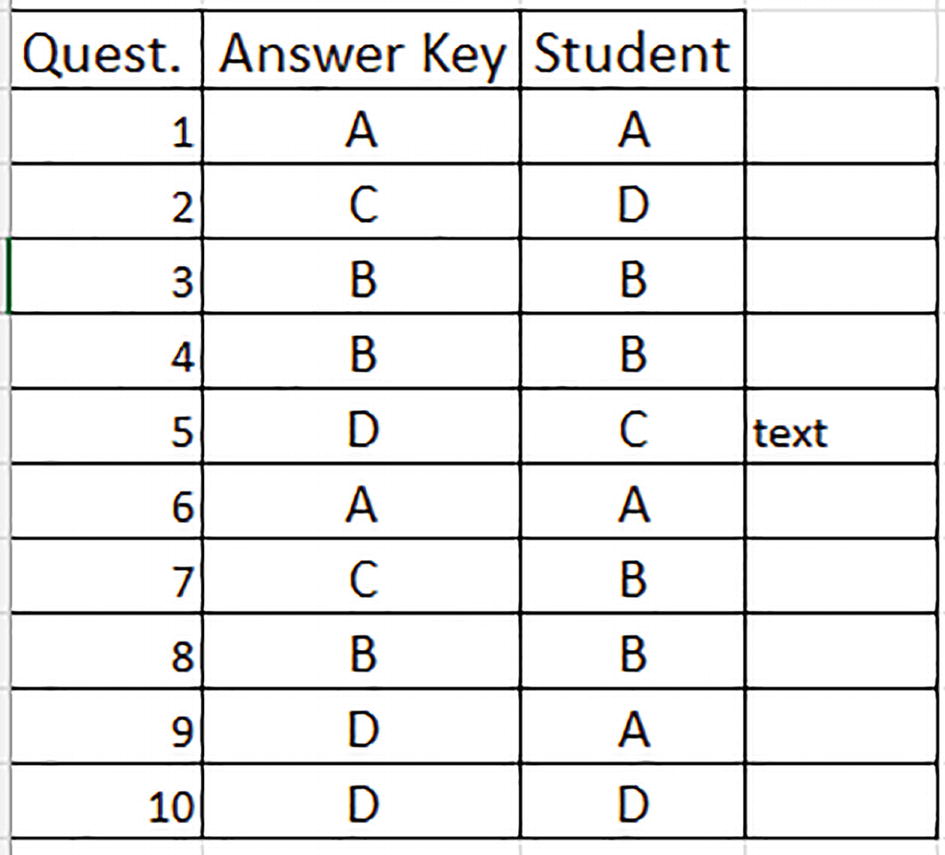
A table of 4 columns and 10 rows. The column labels are, question, answer key, student, and no data. Along with other column entries, column 4 has an entry in row 5, that reads, text.
Unwanted intrusion: text alongside answer 5
=IF(B4:B13=C4:C13,1,0)
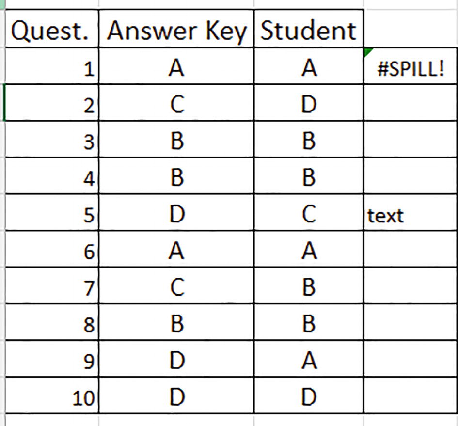
A table of 4 columns and 10 rows. The column labels are, question, answer key, student, and no data. Along with other column entries, 2 entries in column 4 are hash SPILL exclamation mark in row 1 and text in row 5.
All bottled up: the formula won’t spill
You’ve probably surmised what’s happened, and why. The spill range’s values can’t assume their rightful place because the “text” entry in D8 obstructs the spill process. Spilling is an all-or-nothing proposition; if even one of the spilled values is denied entry to its cell, they all are.
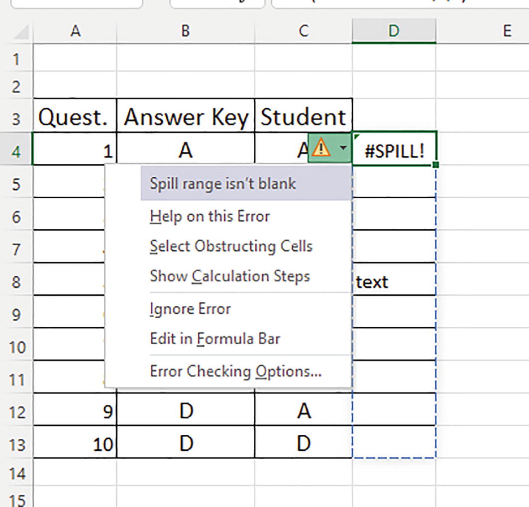
A screenshot of an Excel sheet depicts a table and the cell D 4 selected. It has the data, hash SPILL exclamation mark, and an error window on the left which depicts 7 options. They include spill range isn’t blank, help on this error, select obstructing cells, and others.
Let the data flow with the Select Obstructing Cells option
First, the range earmarked for the spill – in our case, D4:D13 – is surrounded by a dotted border, as the floatie unrolls the Select Obstructing Cells option. Click it, and the cell pointer shoots to cell D8. Now that the offending entry has been pinpointed, just delete it, and the spill range now does its thing.
Of course, you could have identified the obstructing cell on your own; but remember that a single dynamic array formula can unfurl its data across multiple rows and columns at the same time, and so tracing the in-the-way cell(s) might not always be quite so straightforward and evident.
You Can’t Spill on This Table
=IF(B4:B13=C4:C13,1,0)
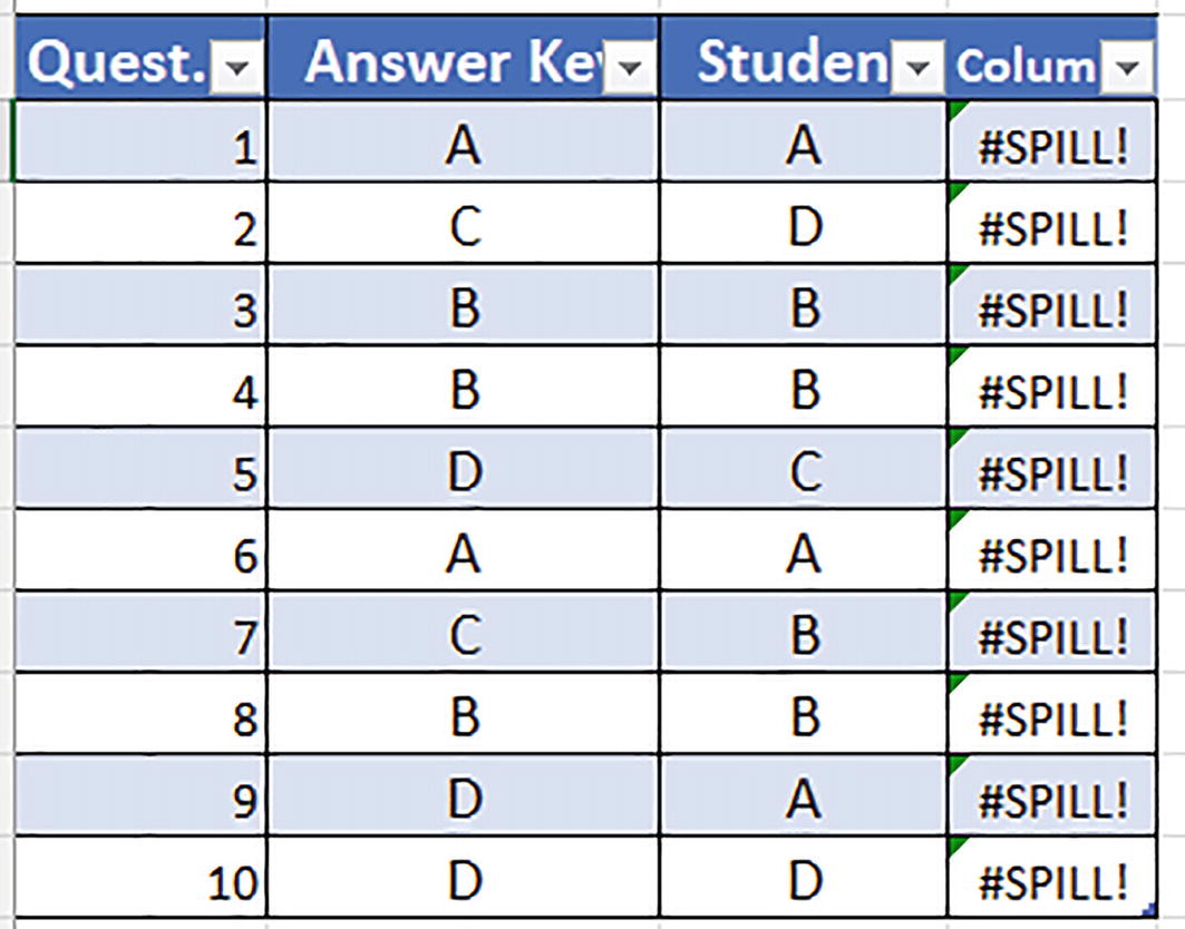
A table of 4 columns and 10 rows. The column labels are, question, answer key, student, and column. All the entries in column 4 read hash SPILL exclamation mark.
Whole lot of spilling going on
Depending on how you write the formula here, the table might render it as =IF([Answer Key]=[@Student],1,0), but that variation won’t matter for our purposes.
The spill sure isn’t working here – but why?
The answer to that question had bothered me for some time, and my initial surmise was to write off a table’s inability to support dynamic arrays as some design gremlin eating away at Excel’s code. But then I experienced a mini-eureka moment and convinced myself that in fact, with one near-theoretical exception, tables can’t work with dynamic array formulas.

A table of 4 columns and 10 rows. The column labels are, question, answer key, student, and no data. Along with other column entries, column 4 has entries from row 1 to row 4.
The Beatles’ next records
But once we reinvent the data into a table, all of its rows become rigorously defined as records, and if you write an ordinary formula to the table, it’s immediately copied to all the records. But remember that our Beatles range formula spills four cells, and so if the table features 100 records, and the Beatle formula and its ensuing spill range were to be copied down a table column, we’d have to contend with 400 results – and 400 cells keyed to 100 records literally doesn’t compute. Because dynamic array formulas spill, their multi-cell output can’t be expected to shoehorn themselves into the records of tables.
There are a few other, far more obscure scenarios in which spills also won’t work, that needn’t concern us here.
But at the same time keep in mind that a dynamic array formula can refer to a table; it just can’t be entered into one – apart from that one unlikely exception.
And that exception to the dynamic array no-table interdiction is, as noted earlier, all but theoretical. If you write a dynamic array formula that yields exactly one record, a table will accommodate it just fine – because the formula has nothing to spill. But given that the dynamic array’s claim to fame is its multi-cell potency, you’re not likely to write, or want to write, such a formula (thanks to Mark of Excel Off the Grid for this pointer).
The # Sign: Weighing In on Its Virtues
=D4#
The pound-sign (or hash mark, depending on the side of the Atlantic on which you live) denotes the cell in which the dynamic array formula is actually written, and writing such a reference will duplicate the formula written to that cell, with all its spilled results.
=SUM(D4#)
will naturally yield 6.
Now of course =SUM(D4:D13) could drum up the same result, but D4# boasts a few advantages: it’s easier and shorter, and more to the point, the pound-sign reference will automatically register any changes to the spill range wrought by the formula.
=SEQUENCE(10)
=SEQUENCE(30)
=COUNT(A3#)
will output 30. But here, even though the COUNT formula is of the one-result type, it can’t be written in previous Excel versions – because those versions have neither the SEQUENCE function nor the pound sign option.
Raising Some More Points About Lifting
To review, the term lifting denotes Excel formulas’ current multi-result potential, now elevated to a veritable default for most of its functions. But there are few more facts about lifting about which you need to know.
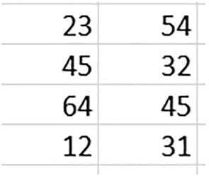
A table of 2 columns and 4 rows. The data are as follows. Row 1: 23, 54. Row 2: 45, 32; Row 3: 64, 45. Row 4: 12, 31.
Times after times – values to be multiplied
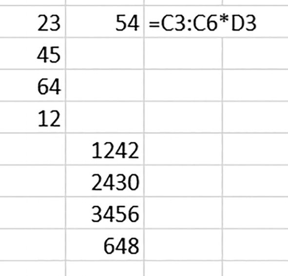
=C3:C6*D3:D6
A table of 3 columns and 4 rows. The data are as follows. Row 1: 23, 54, 1242. Row 2: 45, 32, 1440; Row 3: 64, 45, 2880. Row 4: 12, 31, 372. The formula next to row 1 reads equals C 3 colon C 6 asterisk D 3 colon D 6.
Products of our labors
We’ve again encountered an instance of pairwise lifting, that mode of lifting in which pairs of values are multiplied down their columns. Remember that our initial meet-up with pairwise lifting compared student test responses to an answer key, under the steam of an IF statement. Here, we’ve run through a set of multiplications with the pairs.
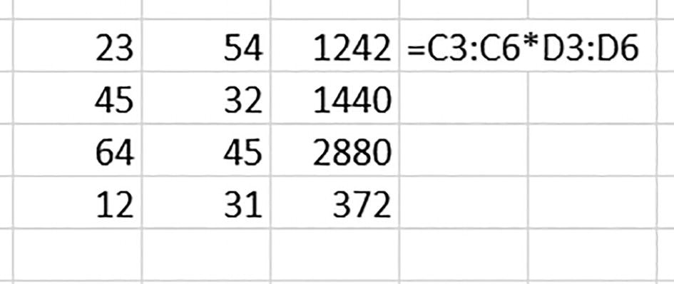
A table of 4 columns and 4 rows. The data are as follows. Row 1: 23, 54, 34, 42228. Row 2: 45, 32, 56, 80640; Row 3: 64, 45, 43, 123840. Row 4: 12, 31, 76, 28272. The formula next to row 1 reads equals C 3 colon C 6 asterisk D 3 colon D 6 asterisk E 3 colon E 6.
Thrice is nice: multiplying trios of values
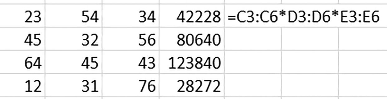
A table of 3 columns and 4 rows. The data are as follows. Row 1: 23, 54, 1242. Row 2: 45, 32, 1440; Row 3: 64, 45, 2880. Row 4: 12, 31, hash N forward slash A. The formula next to row 1 reads equals C 3 colon C 6 asterisk D 3 colon D 5.
An im-paired formula
You see why. The two ranges don’t line up properly – because one bears four cells, the other three. The entry in C6 multiplies itself by a phantom partner, for example, the missing D6, and its formula has no choice but to surrender to an #NA.
Now for a New Angle
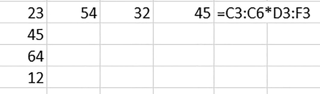
A cropped image of an excel sheet depicts the following entries. Row 1: 23, 54, 32, 45, equals C 3 colon C 6 asterisk D 3 colon F 3. Row 2: 45. Row 3: 64. Row 4: 12.
Reorienting the formula
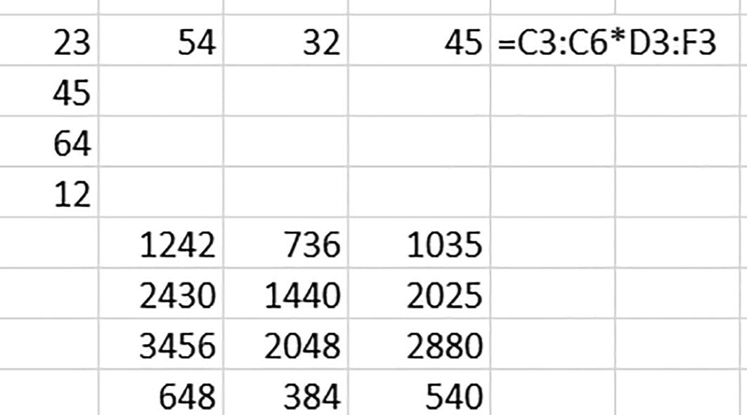
A cropped image of an excel sheet depicts the following entries. Row 1: 23, 54, 32, 45, equals C 3 colon C 6 asterisk D 3 colon F 3. Row 2: 45. Row 3: 64. Row 4: 12. The multiplied values of column 1 with columns 2, 3, and 4 are depicted from row 5 under columns 2, 3, and 4 respectively.
… that one works
Surprise. The second range – which, remember, comprises fewer values than the first one – now stands in a perpendicular relation to the first, and along with that 90-degree shift comes a wholesale rewording of the formula’s marching orders. Now, each value in the first range is multiplied by every value in the second range. For example, the first value (the upper-left cell) in this brand-new spill – 1242 – is nothing else but the product of the first cells of the respective ranges, 23 and 54. Proceeding horizontally, the 736 signifies the product of 23 x 32, and you can probably take it from there.
=D7#
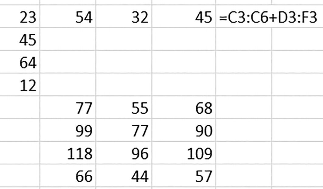
A cropped image of an excel sheet depicts the following entries. Row 1: 23, 54, 32, 45, equals C 3 colon C 6 + D 3 colon F 3. Row 2: 45. Row 3: 64. Row 4: 12. The added values of column 1 with columns 2, 3, and 4 are depicted from row 5 under columns 2, 3, and 4 respectively.
Broadcasting: the addition edition
works too.
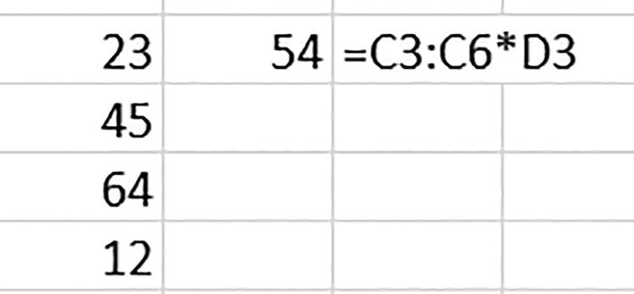
A cropped image of an excel sheet depicts the following entries. Row 1: 23, 54, equals C 3 colon C 6 asterisk D 3. Row 2: 45. Row 3: 64. Row 4: 12.
Going it alone: a one-cell broadcast
A cropped image of an excel sheet depicts the following entries. Row 1: 23, 54, equals C 3 colon C 6 asterisk D 3. Row 2: 45. Row 3: 64. Row 4: 12. The multiplied values of column 1 and column 2 are depicted from row 5 under column 2.
E unum pluribus: out of one (cell), many
But how does it work? My theory is that Excel treats the single value as a narrowest-possible-row, broadcasting it across the four values lining the column.
But terminology aside, you’ll want to understand how broadcasting works, because as we’ll see, it can work for you.
PMT Permutations
=PMT(interest rate divided by number of annual payments,number of payments,loan amount)
=PMT(A2/12,A3,A1)
To explain it: the interest in A2 must be divided by 12, in order to reflect the number of payments per year issued against the 3% rate. A3 simply records the total number of loan payments (12 payments over each of the 2 years, or 24), and the A1 recalls the $10,000 loan sum. The answer: $-429.81, expressed as a negative number simply because the loan debits the borrower’s account. As such, the A1 is commonly entered -A1 in order to restore a positive sign to the result; but that decision is merely presentational.
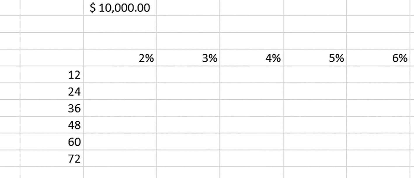
A cropped image of an excel sheet depicts $10000.00 on the top and a matrix of 5 columns and 6 rows below it. The column labels are 2, 3, 4, 5, and 6 in percentage. The row labels are 12, 24, 36, 48, 60, and 72. No entries are filled in the matrix.
The loan arranger
=PMT(G7:K7/12,F8:F13,G4)
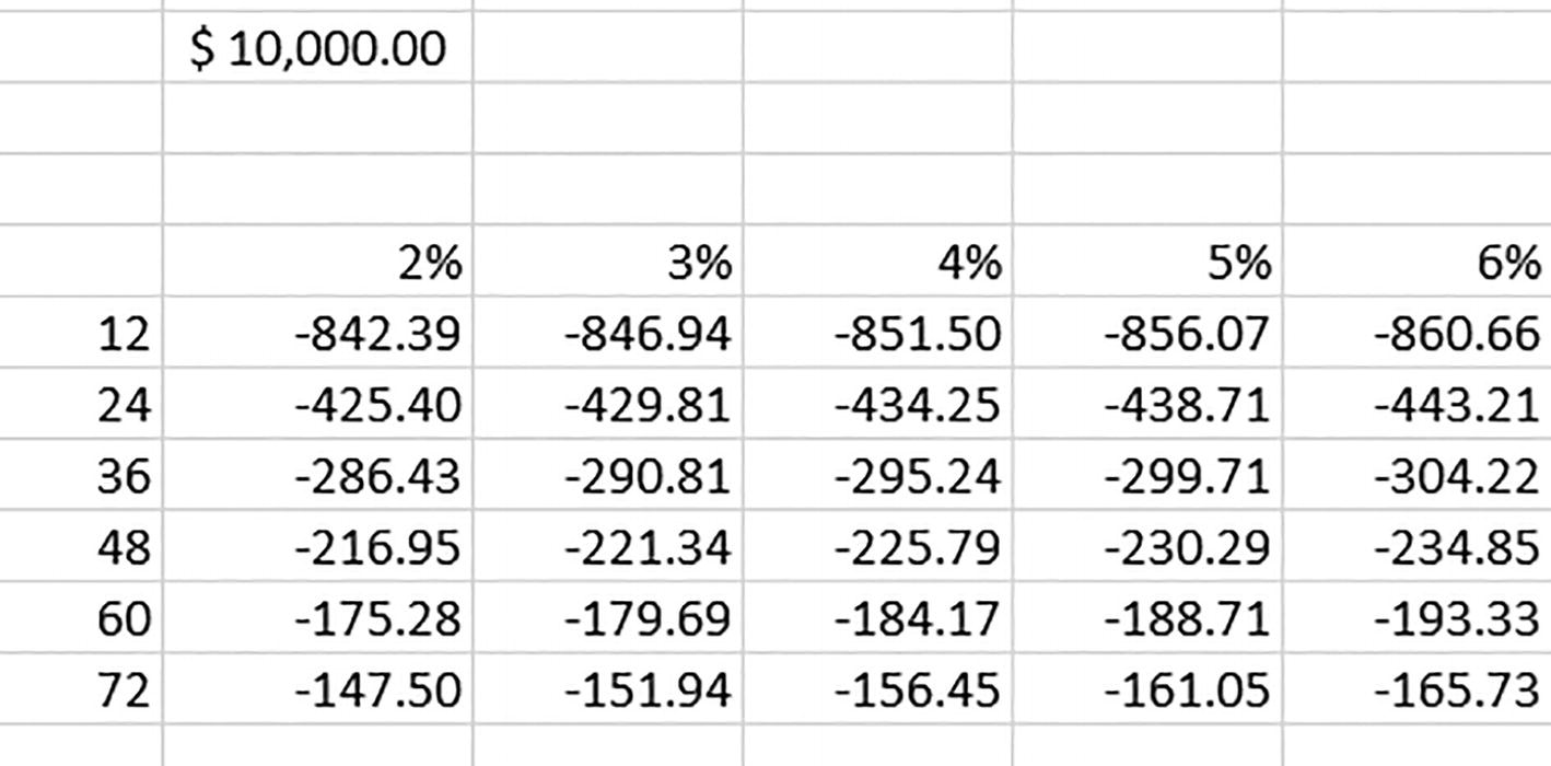
A cropped image of an excel sheet depicts $10000.00 on the top and a loan payment matrix of 5 columns and 6 rows below it. The column labels are 2, 3, 4, 5, and 6 in percentage. The row labels are 12, 24, 36, 48, 60, and 72. Negative values are filled in the matrix.
For your interest: a loan payment matrix, courtesy of one dynamic array formula
Our PMT formula simultaneously inspects every interest rate with the G7:K7/12 argument, and each and every payment frequency via F8:F13. It thus breaks with a conventional PMT by citing ranges instead of single cell references – in other words, it’s a dynamic array formula. The informative upshot, then, all the payment possibilities unfold before the borrower, thanks to that one dynamic array formula.
And whether you realize it or not, our exercise emulates Excel’s ancient Data Table tool, an early array-driven feature with an assortment of moving parts (some of which are rather odd) that, between you and me, I’ve never quite understood (for a Microsoft tutorial on Data Tables look here (https://support.microsoft.com/en-us/office/calculate-multiple-results-by-using-a-data-table-e95e2487-6ca6-4413-ad12-77542a5ea50b)). But never mind; our PMT does the same thing with one formula.
More Lifting – but This Time, Inside a Cell
Now we need to consider one more property of lifting, and it’s an important one. Here’s the demo example, one we can pursue on a blank worksheet. Every Excel character possesses a code number that’s registered by the CODE function. For example, =CODE(“b”) yields 98, while the upper-case variant =CODE(“B”) evaluates to 66. Now suppose that, for whatever reason, we need to learn the code of each of the characters in the word Thursday, which we’ll enter in cell A6. Our challenge is to write one formula that’ll do the job, and in order to achieve that end we’ll need to somehow separate, or extract, each character from Thursday, so that we can peg the proper code to the proper character.
=MID(A6,4,2)
will trot out the result rs for the word Thursday.
MID’s three elements (or “arguments,” as they’re known in the rule book) (1) name the cell on which MID operates, (2) identify the position number of the character from which MID starts its work, and (3) declare the number of characters to be peeled from the cell. Because it’s the r that sits in the fourth position in our Thursday text string, MID commences there and uproots both the r and the s – the 2 characters cited in the last function argument.
=MID(A6,{1,2,3,4,5,6,7,8},1)
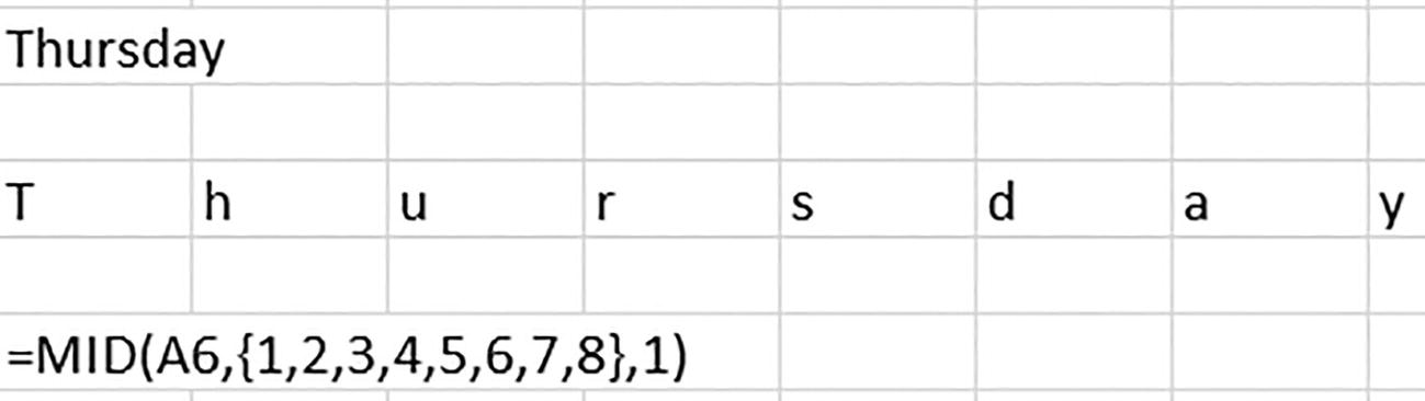
A cropped image of an excel sheet depicts Thursday on the top and letters of Thursday in separate cells below. The formula depicted below is, equals M I D of A 6 comma 1, 2, 3, 4, 5, 6, 7, and 8 within flower braces comma 1.
Confined to their cells; MID extracts each character.
Our MID-based array formula spills its eight results across a horizontal range. MID has in effect applied itself eight times, performing eight character extractions in sequence across its target word, a remarkably nimble feat. And unlike the previous instances of lifting we’ve surveyed to date, the multi-cell output orchestrated here springs from a single cell, and that’s a capability you very much need to keep in mind, and one we need to reexamine.
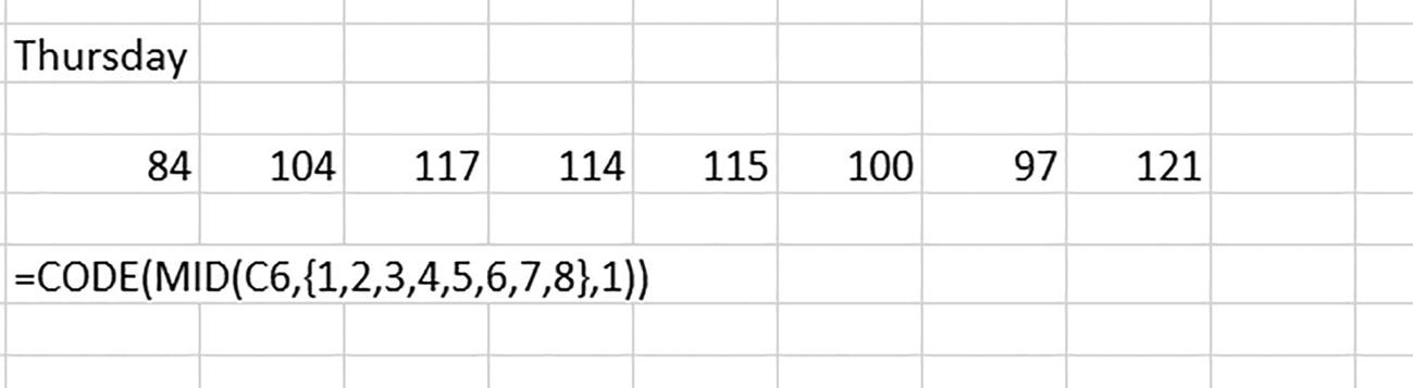
A cropped image of an excel sheet depicts Thursday on the top and 8 numbers in separate cells below. The formula depicted below is, equals CODE of M I D of C 6 comma 1, 2, 3, 4, 5, 6, 7, and 8 within flower braces comma 1.
Thursday, Excel style
Once MID separates the letters, one per cell, the CODE function examines each one and applies its particular code. And all the work has been powered by one formula. That’s real dynamic array power. And remember: neither MID nor CODE is a “new” dynamic array function – but they work dynamically, just the same.
Field Notes: Field and Dataset Names
Now that we’ve battened down our understanding of spills, #s, and the gotta-know essentials of lifting, we can begin to extend a specific welcome to the newest arrivals to the Excel function family – the ones bearing the dynamic array pedigree.
But before we kick off the reviews, a few words about the field and dataset names used here will help clarify the discussions. In the interests of simplicity and training our focus on dynamic arrays, fields will be named after the entries in their header rows unless others indicated. If an exercise requires a reference to the entire dataset, that set will be called All, if it’s static – that is, if the data are to remain as you see them, and not receive any new records. All field names in static datasets – including the global All itself – will work with ranges whose coordinates begin with the row immediately beneath the headers.
Datasets that are prepared to take on new records will have been configured as tables via the standard Ctrl-T keyboard sequence, and they’ll be named Table1, Table2, etc. – but their fields will again simply carry the names of their headers. That latter qualification is necessary, because tables generate default field names exhibiting what Excel calls structured references.
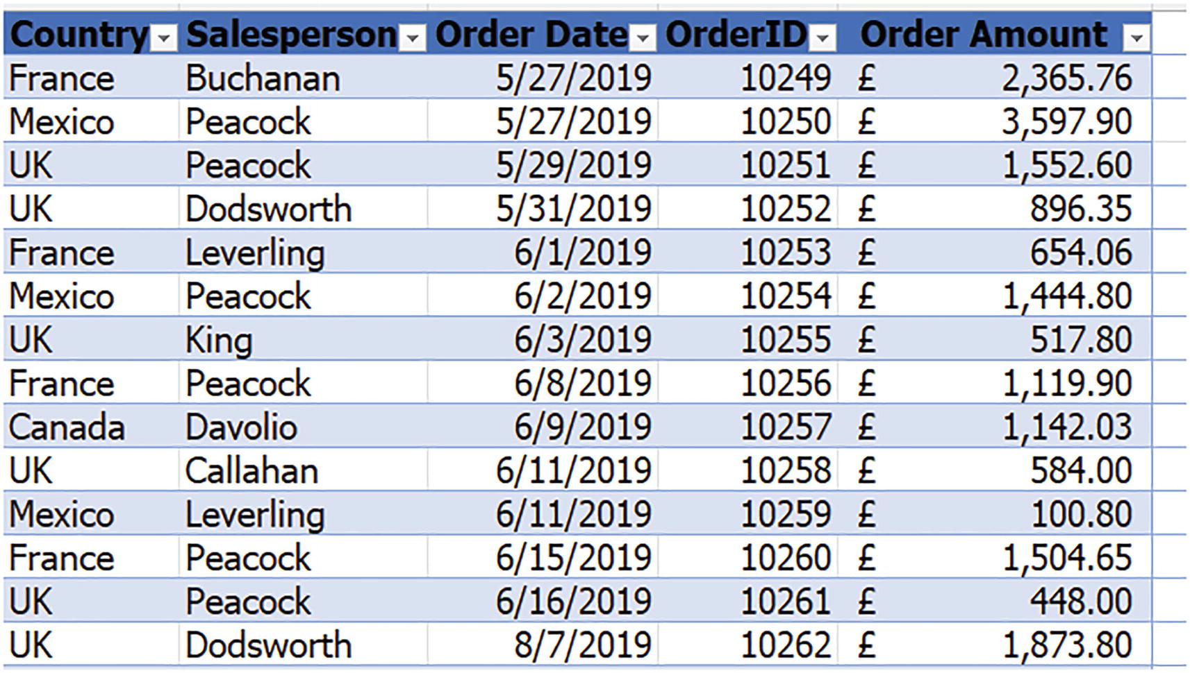
A screenshot depicts a table of 6 columns and 14 rows. The column labels are country, salesperson, order date, order I D, order, and amount.
The table is set
=COUNTA(Table1[Salesperson])
=COUNTA(Salesperson)
Thus, the above field-name type will appear in both kinds of datasets – the static and the table variants.
Click anywhere among the data.
Click Ctrl-A, thus selecting all the dataset cells.
Then click the Formulas tab > Create from Selection command in the Defined Names button group. You’ll see as in Figure 3-20.
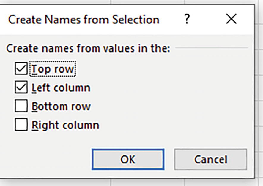
A cropped window titled, create names from selection. The options, create names from values in the top row and left column are checked. O K and the cancel buttons are at the bottom.
An oldie but goodie: the Create from Selection dialog box
Then click Ctrl-T to refurbish the dataset into a table.
Now you’ve gifted yourself with the best of both worlds – you’ve fashioned a table whose fields will automatically register any new records in a formula, and you’ve also allowed yourself to work with conventional, header-based field names.
A final point. From here on, in addition to depicting formulas via the FORMULATEXT function, screenshots will color the cells containing formulas yellow, enhancing clarity.
Next Up
Now that we’ve addressed those necessary preliminaries, it’s time to dive deeply into those dynamic array functions. First up: a function we’ve already glimpsed in passing – SEQUENCE.