
Chapter 4. Data Analysis with pandas
This chapter will introduce you to pandas, the Python Data Analysis Library or—how I like to put it—the Python-based spreadsheet with superpowers. It’s so powerful that some of the companies that I worked with have managed to get rid of Excel completely by replacing it with a combination of Jupyter notebooks and pandas. As a reader of this book, however, I assume you will keep Excel, in which case pandas will serve as an interface for getting data in and out of Excel. pandas is such a great library because it makes tasks that are particularly painful in Excel easier, faster and less error-prone. Some of these tasks include getting big datasets from external sources and working with statistics, time series and interactive charts. pandas’ most important superpowers are vectorization and data alignment. Vectorization allows you to write concise, array-based code and the data alignment capabilities make sure that there is no mismatch of data when you work with multiple datasets.
This chapter covers the whole journey of performing data analysis with pandas. It introduces the data structures DataFrame and Series and explains how to prepare and clean data by selecting subsets, performing calculations or combining multiple DataFrames. After that, you will learn how to make sense out of bigger datasets by calculating descriptive statistics on aggregated data and by visualizing the results. The chapter moves on with explaining how to import and export data and concludes with a longer section about time series analysis. Before we dive into pandas though, I will start with the basics of NumPy, which pandas is built upon. Even if we will hardly use NumPy directly in this book, knowing its basics will make it easier for you to get started with pandas.
Foundations: NumPy
As you may recall from Chapter 1, NumPy is the core package for scientific computing in Python, providing support for array-based calculations and linear algebra. As NumPy is the backbone of pandas, I am going to introduce its basics briefly in this section: after explaining what a NumPy’s array is, I am going to introduce vectorization and broadcasting, two important concepts that allow you to write concise mathematical code and that you will find again in pandas. After that, we’re going to see why NumPy offers special functions called universal functions before we wrap this section up by learning how to get and set values of an array and by explaining the difference between a view and a copy of a NumPy array.
NumPy Array
To perform array-based calculations with nested lists, as we met them in the last chapter, you would have to write some sort of loop. For example, to add a number to every element in a nested list, you can use the following nested list comprehension:
In[1]:matrix=[[1,2,3],[4,5,6],[7,8,9]]
In[2]:[[i+1foriinrow]forrowinmatrix]
Out[2]:[[2,3,4],[5,6,7],[8,9,10]]
This isn’t very readable and more importantly, if you do this with big arrays, looping through each element becomes very slow. Depending on your use case and the size of the arrays, calculating with NumPy arrays instead of Python lists can be anywhere between a couple of times to up to a hundred times faster. NumPy achieves this by using code that is written in a compiled programming language like C or Fortran. A NumPy array is an N-dimensional array for homogenous data called ndarray. Homogenous means that all elements in the array need to have the same data type. Most commonly, you are dealing with one- and two-dimensional arrays of floats as schematically displayed in Figure 4-1.
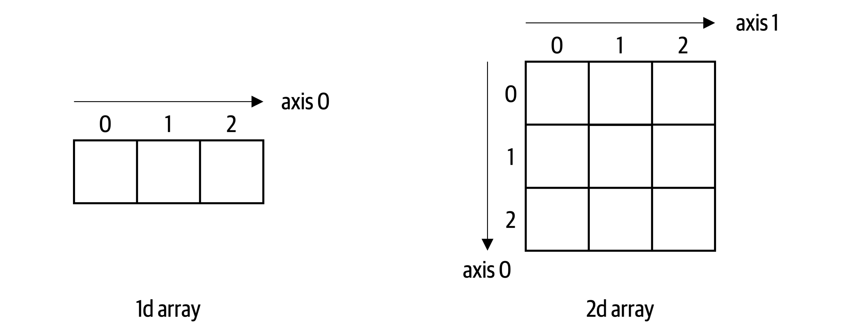
Figure 4-1. A one-dimensional and two-dimensional NumPy array
Let’s create a one- and two-dimensional array to work with throughout this section:
In[3]:importnumpyasnp
In[4]:# Constructing an array with a simple list results in a 1d arrayarray1=np.array([10,100,1000.])
In[5]:# Constructing an array with a nested list results in a 2d arrayarray2=np.array([[1.,2.,3.],[4.,5.,6.]])
It’s important to note the difference between a one- and two-dimensional array: A one-dimensional array has only one axis and hence does not have an explicit column or row orientation. While this behaves like arrays in VBA, you may have to get used to it if you come from a language like MATLAB, where one-dimensional arrays always have a column or row orientation. Even if there are only integers in the array except for one float, the homogeneity of NumPy arrays forces the data type of the array to be float64 which is capable of accommodating all elements:
In[6]:array1.dtype
Out[6]:dtype('float64')
Since dtype gives you back float64 and not float which we met in the last chapter, you can probably guess that NumPy uses its own numerical data types which are more granular than Python’s data types. This usually isn’t an issue though as most of the time, conversion between the different data types in Python and NumPy happens automatically. If you ever need to explicitly convert a NumPy data type to a Python data type, it’s enough to use the Python constructor, e.g. float(array1[0]). You can see a full list of NumPy’s data types in the NumPy docs. Working with NumPy arrays allows you to write simple code to perform array-based calculations as you will see next.
Vectorization and Broadcasting
If you build the sum of a scalar1 and a NumPy array, NumPy will perform an element-wise operation. You don’t have to loop through the elements yourself. The NumPy community refers to this as vectorization. It allows you to write concise code practically representing the mathematical notation:
In[7]:array2+1
Out[7]:array([[2.,3.,4.],[5.,6.,7.]])
The same principle applies when you work with two-dimensional arrays: NumPy performs the operation element-wise:
In[8]:array2*array2
Out[8]:array([[1.,4.,9.],[16.,25.,36.]])
When you use two arrays with different shapes in an arithmetic operation, NumPy extends—if possible—the smaller array automatically across the larger array so that their shapes become compatible. This is called broadcasting:
In[9]:array2*array1
Out[9]:array([[10.,200.,3000.],[40.,500.,6000.]])
To perform matrix multiplications or dot products, use the @ operator (.T is a shortcut for the transpose method):
In[10]:array2@array2.T
Out[10]:array([[14.,32.],[32.,77.]])
You know now that arrays perform arithmetic operations element-wise, but how can you apply a function on every element in an array? This is what universal functions are here for.
Universal Functions (ufunc)
Universal functions (ufunc) work on every element in a NumPy array. For example, if you use Python’s standard square root function from the math module on a NumPy array, you will get an error:
In[11]:importmathmath.sqrt(array2)# this will raise en Error
---------------------------------------------------------------------------
TypeError                                 Traceback (most recent call last)
<ipython-input-11-97836c28dfe9> in <module>
      1 import math
----> 2 math.sqrt(array2)  # this will raise en Error

TypeError: only size-1 arrays can be converted to Python scalars
You could, of course, write a nested loop to get the square root of every element, then build a NumPy array again from the result:
In[12]:np.array([[math.sqrt(i)foriinrow]forrowinarray2])
Out[12]:array([[1.,1.41421356,1.73205081],[2.,2.23606798,2.44948974]])
This will work in cases where NumPy doesn’t offer a ufunc and the array is small enough. However, if NumPy has a ufunc, use it as it will be much faster with big arrays—apart from being easier to type and read:
In[13]:np.sqrt(array2)
Out[13]:array([[1.,1.41421356,1.73205081],[2.,2.23606798,2.44948974]])
Some of NumPy’s ufuncs, like sum, are additionally available as array methods: if you want the sum of each column, you can do:
In[14]:array2.sum(axis=0)# returns a 1d array
Out[14]:array([5.,7.,9.])
axis=0 refers to the axis along the rows while axis=1 refers to the axis along the columns as depicted in Figure 4-1. You will meet more NumPy ufuncs throughout this book when we use them with pandas DataFrames.
Up to this point, we’ve always worked with whole arrays. The next topic shows you how you select elements from an array to get and set values.
Getting and Setting Array Elements
In the last chapter, I showed you how you can use indexing and slicing with lists to get access to specific elements. When dealing with nested lists like matrix from the first example in this chapter, you can use chained indexing: to get the first element from the first row, you can write matrix[0][0]. With NumPy arrays, however, you provide the index and slice arguments for both dimensions in a single pair of square brackets:
myarray[row_selection,column_selection]
For one-dimensional arrays, this simplifies to myarray[selection]. When you select a single element, you will get back a scalar, otherwise, you will get back a one- or two-dimensional array. Remember that slice notation uses a start index (included) and an end index (excluded) with a colon in between as in start:end. By leaving away the start and end index, you are left with a colon, which therefore stands for all rows or all columns in a two-dimensional array. Let’s get a feeling for how this works with the following example—they are also visualized in Figure 4-2:
In[15]:array1[2]# returns a scalar
Out[15]:1000.0
In[16]:array2[0,0]# returns a scalar
Out[16]:1.0
In[17]:array2[:,1:]# returns a 2d array
Out[17]:array([[2.,3.],[5.,6.]])
In[18]:array2[:,1]# returns a 1d array
Out[18]:array([2.,5.])
In[19]:array2[1,:2]# returns a 1d array
Out[19]:array([4.,5.])

Figure 4-2. Selecting elements of a NumPy array
Remember, by slicing a column or row of a two-dimensional array, you end up with a one-dimensional array, not with a two-dimensional column or row vector.
So far, I have constructed the sample arrays by hand, i.e. by providing numbers in a list. If you need bigger arrays, that is not practical anymore. Fortunately, NumPy offers a few useful functions to construct arrays.
Useful Array Constructors
NumPy offers a few ways to construct arrays that will be helpful to create pandas DataFrames, too. To easily create big arrays, you can use arange. This stands for array range and is similar to range that we met in the previous chapter—with the difference that it returns a NumPy array. Combining it with reshape allows you to quickly generate an array with the desired dimensions:
In[20]:np.arange(10).reshape(2,5)# 2 rows, 5 columns
Out[20]:array([[0,1,2,3,4],[5,6,7,8,9]])
Another common need, for example for Monte Carlo simulations, is to generate arrays of normally distributed pseudo-random numbers. NumPy makes this easy:
In[21]:np.random.randn(2,3)# 2 rows, 3 columns
Out[21]:array([[0.20156739,0.40499128,0.14961916],[0.0494493,1.425759,0.12646884]])
I will show you later in this chapter how you can turn these arrays into pandas DataFrames.
Now that you can create big arrays, it’s good to know that NumPy returns views and not copies when you slice an array—this keeps memory consumption low. How it works exactly is what I’ll explain next.
View vs. Copy
NumPy arrays return views when you slice them. This means that you are working with a subset of the original array without copying the data. Setting a value on a view will therefore also change the original array:
In[22]:array2
Out[22]:array([[1.,2.,3.],[4.,5.,6.]])
In[23]:subset=array2[:,:2]subset
Out[23]:array([[1.,2.],[4.,5.]])
In[24]:subset[0,0]=1000
In[25]:subset
Out[25]:array([[1000.,2.],[4.,5.]])
In[26]:array2
Out[26]:array([[1000.,2.,3.],[4.,5.,6.]])
If you want to work with an independent array, you have to copy it first:
array2_copy=array2.copy()
This was a short introduction to the most important NumPy concepts. To wrap this section up, I am giving you a few reasons why we will use pandas for data analysis rather than NumPy directly.
Limitations with NumPy
While NumPy is an incredibly powerful library, there are two main issues when you want to use it for data analysis:
-
The whole NumPy array needs to be of the same data type. This, for example, means that you can’t perform any of the arithmetic operations we did in this section when your array contains a mix of text and numbers. As soon as text is involved, the array will have the data type
objectwhich will not allow mathematical operations. -
Using NumPy arrays for data analysis makes it hard to know what each column or row refers to as you typically select columns via their position as in
myarray[:, 1].
pandas has solved these issues by providing smarter data structures on top of NumPy arrays. What they are and how they work is the topic of the next section.
DataFrame and Series
DataFrame and Series are the core data structures in pandas. In this section, I am introducing them with a focus on the main components of a DataFrame: index, columns and data. A DataFrame is similar to a two-dimensional NumPy array but it has additional column and row labels and each column can hold different data types. By extracting a single column or row from a DataFrame, you get a one-dimensional Series. Again, a Series is similar to a one-dimensional NumPy array with labels. When you look at the DataFrame in Figure 4-3, it won’t take a lot of imagination to see that DataFrames are going to be your Python-based spreadsheets.

Figure 4-3. A pandas Series and DataFrame
Let’s create a simple DataFrame representing participants of an online course. After importing pandas, we create a DataFrame by providing the data in the form of a nested list, along with values for columns and index:
In[27]:importpandasaspddata=[['Mark',55,'Italy',4.5,'Europe'],['John',33,'USA',6.7,'America'],['Tim',41,'USA',3.9,'America'],['Jenny',12,'Germany',9.0,'Europe']]df=pd.DataFrame(data=data,columns=['name','age','country','score','continent'],index=[1001,1000,1002,1003])df
Out[27]:nameagecountryscorecontinent1001Mark55Italy4.5Europe1000John33USA6.7America1002Tim41USA3.9America1003Jenny12Germany9.0Europe
If you run this in a Jupyter notebook, the DataFrames will be nicely formatted as HTML table and when you hover over a row, it will be highlighted. By calling the info method, you will get some basic information, most importantly the number of data points and the data types for each column:
In[28]:df.info()
<class 'pandas.core.frame.DataFrame'>
Int64Index: 4 entries, 1001 to 1003
Data columns (total 5 columns):
 #   Column     Non-Null Count  Dtype
---  ------     --------------  -----
 0   name       4 non-null      object
 1   age        4 non-null      int64
 2   country    4 non-null      object
 3   score      4 non-null      float64
 4   continent  4 non-null      object
dtypes: float64(1), int64(1), object(3)
memory usage: 192.0+ bytes
If you are just interested in the data type of your columns, you can also run df.dtypes instead. Columns with strings or mixed data types will have the data type object 2. Let us now have a closer look at the index and columns of a DataFrame.
Index
The row labels of a DataFrame are called index. If you don’t have a meaningful index, you can leave it away when constructing a DataFrame. pandas will then automatically create an integer index starting at zero. An index will allow pandas to lookup data faster and is essential for many common operations like combining two DataFrames. You can get information about the index like this:
In[29]:df.index
Out[29]:Int64Index([1001,1000,1002,1003],dtype='int64')
If it makes sense, you can give the index a name. In our example, let’s assume the index is the user ID:
In[30]:df.index.name='user_id'df
Out[30]:nameagecountryscorecontinentuser_id1001Mark55Italy4.5Europe1000John33USA6.7America1002Tim41USA3.9America1003Jenny12Germany9.0Europe
Note that unlike the index of a database, a DataFrame index can have duplicates, but looking up values may be slower in that case. You can turn an index into a regular column by using reset_index and you can set a new index by using set_index. If you don’t want to lose your existing index when setting a new one, make sure to reset it first:
In[31]:# Turns the index into a column,# replacing the index with the default indexdf.reset_index()
Out[31]:user_idnameagecountryscorecontinent01001Mark55Italy4.5Europe11000John33USA6.7America21002Tim41USA3.9America31003Jenny12Germany9.0Europe
In[32]:# Turns 'user_id' into a regular column and# makes the column 'name' the indexdf.reset_index().set_index('name')
Out[32]:user_idagecountryscorecontinentnameMark100155Italy4.5EuropeJohn100033USA6.7AmericaTim100241USA3.9AmericaJenny100312Germany9.0Europe
By doing df.reset_index().set_index('name'), you are using method chaining: since reset_index() returns a DataFrame, you can directly call another DataFrame method without having to write out the intermediate result first.
DataFrame Methods Return Copies
Whenever you call a method on a DataFrame like df.reset_index(), you will get back a copy of the DataFrame with that method applied, leaving the original DataFrame untouched. If you’d like to change the original DataFrame, you have to assign the return value back to the original variable like this: df = df.reset_index(). This means that our variable df is still holding its original data.
To change the index, you can use the reindex method:
In[33]:df.reindex([999,1000,1001,1004])
Out[33]:nameagecountryscorecontinentuser_id999NaNNaNNaNNaNNaN1000John33.0USA6.7America1001Mark55.0Italy4.5Europe1004NaNNaNNaNNaNNaN
This is a first example of data alignment at work as reindex will take over all rows that match the new index and will introduce rows with missing values (NaN) where no information exists. Index elements that you leave away will be dropped. I will introduce NaN properly a little later in this chapter. Finally, to sort an index, use the sort_index method:
In[34]:df.sort_index()
Out[34]:nameagecountryscorecontinentuser_id1000John33USA6.7America1001Mark55Italy4.5Europe1002Tim41USA3.9America1003Jenny12Germany9.0Europe
If, instead, you want to sort the rows by one or more columns instead, use sort_values:
In[35]:df.sort_values(['name','age'])
Out[35]:nameagecountryscorecontinentuser_id1003Jenny12Germany9.0Europe1000John33USA6.7America1001Mark55Italy4.5Europe1002Tim41USA3.9America
The sample shows how to sort first by name, then by age. If you wanted to sort by only one column, you could provide the column name as string: df.sort_values('name').
That’s enough about the index for the moment. Let’s now turn our attention to its horizontal equivalent, the DataFrame columns!
Columns
To get information about the columns of a DataFrame, do:
In[36]:df.columns
Out[36]:Index(['name','age','country','score','continent'],dtype='object')
Again, if you don’t provide any column names when constructing a DataFrame, pandas will number the columns starting at zero. Like with the index, you can assign a name to the columns:
In[37]:df.columns.name='properties'df
Out[37]:propertiesnameagecountryscorecontinentuser_id1001Mark55Italy4.5Europe1000John33USA6.7America1002Tim41USA3.9America1003Jenny12Germany9.0Europe
If you don’t like the column names, you can rename them:
In[38]:df.rename(columns={'name':'First Name','age':'Age'})
Out[38]:propertiesFirstNameAgecountryscorecontinentuser_id1001Mark55Italy4.5Europe1000John33USA6.7America1002Tim41USA3.9America1003Jenny12Germany9.0Europe
If you want to delete columns, you can use the following syntax (the sample shows you how to drop columns and indices at the same time):
In[39]:df.drop(columns=['name','country'],index=[1000,1003])
Out[39]:propertiesagescorecontinentuser_id1001554.5Europe1002413.9America
The columns and the index of a DataFrame are both represented by an Index object, so you can change your columns into rows and vice versa by transposing your DataFrame:
In[40]:df.T# shortcut for df.transpose()
Out[40]:user_id1001100010021003propertiesnameMarkJohnTimJennyage55334112countryItalyUSAUSAGermanyscore4.56.73.99continentEuropeAmericaAmericaEurope
To conclude, if you would like to reorder the columns of a DataFrame, select them in the desired order:
In[41]:df.loc[:,['continent','country','name','age','score']]
Out[41]:propertiescontinentcountrynameagescoreuser_id1001EuropeItalyMark554.51000AmericaUSAJohn336.71002AmericaUSATim413.91003EuropeGermanyJenny129.0
This last example needs quite a few explanations: everything about loc and how data selection works is the topic of the next section.
Data Manipulation
Real-world data hardly gets served on a silver platter, so before you can work with it, you need to do some data manipulation to clean it and bring it into a digestible form. Accordingly, this section starts with how to select data from a DataFrame, how to change it and how to deal with missing and duplicate data. I’ll then show you how to perform calculations with DataFrames and how to work with text data. I will finish this section by explaining when pandas returns a view vs. a copy of the data. Quite a few concepts in this section are related to what we have already seen with NumPy arrays.
Selecting Data
Let’s start with accessing data by label and position before looking at other methods including boolean indexing and selecting data by using a MultiIndex.
Selecting by label
The most common way of accessing the data of a DataFrame is by referring to its labels. Use the attribute loc, which stands for location, to specify which rows and columns you want to retrieve:
df.loc[row_selection,column_selection]
loc supports the slice notation and therefore accepts a colon to select all rows or columns, respectively. Additionally, you can provide lists with labels as well as a single column or row name. Have a look at Table 4-1 to see a few examples of how you can select different parts from our sample DataFrame df.
| Selection | Return Data Type | Example |
|---|---|---|
Single value |
Scalar |
|
One column (1d) |
Series |
|
One column (2d) |
DataFrame |
|
Multiple columns |
DataFrame |
|
Range of columns |
DataFrame |
|
One row (1d) |
Series |
|
One row (2d) |
DataFrame |
|
Multiple rows |
DataFrame |
|
Range of rows |
DataFrame |
|
Label Slicing Has Closed Intervals
Using slice notation with labels is inconsistent with respect to how everything else in Python and pandas works: they include the upper end.
Applying our knowledge from Table 4-1, let’s use loc to select scalars, Series and DataFrames:
In[42]:df.loc[1000,'name']# Returns a Scalar
Out[42]:'John'
In[43]:df.loc[[1000,1002],'name']# Returns a Series
Out[43]:user_id1000John1002TimName:name,dtype:object
In[44]:df.loc[:1002,['name','country']]# Returns a DataFrame
Out[44]:propertiesnamecountryuser_id1001MarkItaly1000JohnUSA1002TimUSA
It’s important that you understand the difference between a DataFrame with one or more columns and a Series: even with a single column, DataFrames are two-dimensional, while Series are one-dimensional. Both, DataFrame and Series, have an index, but only the DataFrame has column headers. When you select a column as Series, the column header becomes the name of the Series. Many functions or methods will work on both, Series and DataFrame, but when you perform arithmetic calculations, the behavior differs: with DataFrames, pandas aligns the data according to the column headers—more about that will follow later in this chapter.
Shortcut for Column Selection
Since selecting columns is such a common operation, pandas offers a shortcut. Instead of:
df.loc[:,column_selection]
you can write:
df[column_selection]
For example, to select a Series from our sample DataFrame, you can do df['country'] and to select a DataFrame with multiple columns, you can do df[['name', 'country']].
Selecting by position
Selecting a subset of a DataFrame by position corresponds to what we did at the beginning of this chapter with NumPy arrays. With DataFrames, however, you have to use the iloc attribute which stands for integer location:
df.iloc[row_selection,column_selection]
When using slices, you deal with the standard half-open intervals. Table 4-2 gives you the same cases as we previously looked at with loc:
| Selection | Return Data Type | Example |
|---|---|---|
Single value |
Scalar |
|
One column (1d) |
Series |
|
One column (2d) |
DataFrame |
|
Multiple columns |
DataFrame |
|
Range of columns |
DataFrame |
|
One row (1d) |
Series |
|
One row (2d) |
DataFrame |
|
Multiple rows |
DataFrame |
|
Range of rows |
DataFrame |
|
Here is how you use iloc—again with the same samples that we used with loc before:
In[45]:df.iloc[0,0]# Returns a Scalar
Out[45]:'Mark'
In[46]:df.iloc[[0,2],1]# Returns a Series
Out[46]:user_id100155100241Name:age,dtype:int64
In[47]:df.iloc[:3,[0,2]]# Returns a DataFrame
Out[47]:propertiesnamecountryuser_id1001MarkItaly1000JohnUSA1002TimUSA
Selecting data by label and position are not the only means to access a subset of your DataFrame. Another important way is to use boolean indexing—let’s see how it works!
Selecting by boolean indexing
Boolean indexing refers to selecting subsets of a DataFrame with the help of a Series or a DataFrame whose data consist of only True or False. Boolean Series are used to select specific columns and rows of a DataFrame while boolean DataFrames are used to select specific values across a whole DataFrame. Most commonly you will use boolean indexing to filter the rows of a DataFrame. Think of it as the AutoFilter functionality in Excel. The easiest way to filter the rows of a DataFrame is by using one or more boolean Series. For example, to filter your DataFrame so it only shows people who live in the USA and are older than 40 years, you can write:
In[48]:tf=(df['age']>40)&(df['country']=='USA')tf# true/false
Out[48]:user_id1001False1000False1002True1003Falsedtype:bool
In[49]:df.loc[tf,:]
Out[49]:propertiesnameagecountryscorecontinentuser_id1002Tim41USA3.9America
There are two things I need to explain here. First, due to technical reasons, you can’t use Python’s boolean operators with DataFrames. Instead, you need to use the symbols as shown in Table 4-3.
| Basic Python Data Types | DataFrames and Series |
|---|---|
|
|
|
|
|
|
Second, if you have more than one condition, make sure to put every boolean expression in between parentheses so operator precedence doesn’t get in your way: for example, & has higher operator precedence than ==. Therefore, without parentheses, the expression from the sample would be interpreted as df['age'] > (40 & df['country']) == 'USA'. If you want to filter the index, you can refer to it as df.index:
In[50]:df.loc[df.index>1001,:]
Out[50]:propertiesnameagecountryscorecontinentuser_id1002Tim41USA3.9America1003Jenny12Germany9.0Europe
For what you would use the in operator with basic Python data structures like lists, you can use isin with a Series. This way you can filter your DataFrame to participants from Italy and Germany:
In[51]:df.loc[df['country'].isin(['Italy','Germany']),:]
Out[51]:propertiesnameagecountryscorecontinentuser_id1001Mark55Italy4.5Europe1003Jenny12Germany9.0Europe
While you use loc to provide a boolean Series, DataFrames offer a special syntax without loc to select values given the full DataFrame of booleans:
df[boolean_df]
This is especially helpful if you have DataFrames that consist of only numbers. Providing a DataFrame of booleans returns the DataFrame with NaN wherever the boolean DataFrame is False. Again, a more detailed discussion of NaN will follow shortly.
In[52]:numbers=pd.DataFrame({'A':[1.3,3.2],'B':[-4.2,-2.1],'C':[-5.5,3.1]})numbers
Out[52]:ABC01.3-4.2-5.513.2-2.13.1
In[53]:numbers<2
Out[53]:ABC0TrueTrueTrue1FalseTrueFalse
In[54]:numbers[numbers<2]
Out[54]:ABC01.3-4.2-5.51NaN-2.1NaN
Note that in this example, I have used a dictionary to construct a new DataFrame—this is often convenient if the data is already existing in that form. Boolean indexing is most commonly used to filter out specific values like e.g. outliers. To wrap up the data selection part, I will introduce a special type of index, the MultiIndex.
Selecting by using a MultiIndex
A MultiIndex is an index with more than one level. It allows you to hierarchically group your data and gives you easy access to subsets. For example, if you set the index of our sample DataFrame df to a combination of continent and country, you can easily select all rows with a certain continent:
In[55]:# MultiIndex need to be sorteddf_multi=df.reset_index().set_index(['continent','country'])df_multi=df_multi.sort_index()df_multi
Out[55]:propertiesuser_idnameagescorecontinentcountryAmericaUSA1000John336.7USA1002Tim413.9EuropeGermany1003Jenny129.0Italy1001Mark554.5
In[56]:df_multi.loc['Europe',:]
Out[56]:propertiesuser_idnameagescorecountryGermany1003Jenny129.0Italy1001Mark554.5
Note that pandas prettifies the output of a MultiIndex by not repeating the leftmost index level (the continents) for each row. Instead, it only prints the continent when it changes. Selecting over multiple index levels is done by providing a tuple:
In[57]:df_multi.loc[('Europe','Italy'),:]
Out[57]:propertiesuser_idnameagescorecontinentcountryEuropeItaly1001Mark554.5
If you want to selectively reset part of a MultiIndex, you can provide the level as argument. Zero is the first column from the left:
In[58]:df_multi.reset_index(level=0)
Out[58]:propertiescontinentuser_idnameagescorecountryUSAAmerica1000John336.7USAAmerica1002Tim413.9GermanyEurope1003Jenny129.0ItalyEurope1001Mark554.5
While I won’t make extensive use of MultiIndex in this book, there are certain operations like groupby, which will cause pandas to return a DataFrame with a MultiIndex, so it’s good to know what it is. We will meet groupby later in this chapter.
Now that you know how to select data, it’s time to learn how you can change data.
Setting Data
The easiest way to change the data of a DataFrame is by assigning values to certain elements using the loc or iloc attributes. This is the starting point of this section before we turn to other ways of manipulating existing DataFrames: replacing values and adding new columns.
Setting data by label or position
When you call DataFrame methods like df.reset_index(), the method will always be applied to a copy of the original DataFrame. However, when working with the loc and iloc attributes, you are accessing the DataFrame directly. Using them to assign values accordingly changes the original DataFrame. Since I want to leave the original DataFrame df untouched, I am working with a copy here that I call df2. If you want to change a single value, you can do:
In[59]:df2=df.copy()
In[60]:df2.loc[1000,'name']='JOHN'df2
Out[60]:propertiesnameagecountryscorecontinentuser_id1001Mark55Italy4.5Europe1000JOHN33USA6.7America1002Tim41USA3.9America1003Jenny12Germany9.0Europe
You can also change multiple values at the same time. For example, to change the score of the users with ID 1000 and 1001, you can use a list:
In[61]:df2.loc[[1000,1001],'score']=[3,4]df2
Out[61]:propertiesnameagecountryscorecontinentuser_id1001Mark55Italy4.0Europe1000JOHN33USA3.0America1002Tim41USA3.9America1003Jenny12Germany9.0Europe
Changing data by position via iloc works the same way.
Setting data by boolean indexing
Boolean indexing, which we used to filter rows, can also be used to assign values in a DataFrame. Imagine that you need to anonymize all names of people who are below 20 years old or from the USA:
In[62]:tf=(df2['age']<20)|(df2['country']=='USA')df2.loc[tf,'name']='xxx'df2
Out[62]:propertiesnameagecountryscorecontinentuser_id1001Mark55Italy4.0Europe1000xxx33USA3.0America1002xxx41USA3.9America1003xxx12Germany9.0Europe
Sometimes, you have a dataset where you need to replace certain values across the board, i.e. not specific to certain columns. In that case, you can make use of the special syntax again and provide the whole DataFrame with booleans like this:
In[63]:numbers2=numbers.copy()numbers2
Out[63]:ABC01.3-4.2-5.513.2-2.13.1
In[64]:numbers2[numbers2<2]=0numbers2
Out[64]:ABC00.00.00.013.20.03.1
Setting data by replacing values
If you want to replace a certain value across your entire DataFrame or selected columns, you can do this by using the replace method:
In[65]:df.replace('USA','U.S.')
Out[65]:propertiesnameagecountryscorecontinentuser_id1001Mark55Italy4.5Europe1000John33U.S.6.7America1002Tim41U.S.3.9America1003Jenny12Germany9.0Europe
If, instead, you only want to act on the country column, use this syntax instead:
df.replace({'country':{'USA':'U.S.'}})
Setting data by adding a new column
You can add a new column by assigning values to a new column name. You can assign a scalar or e.g. a list:
In[66]:df2.loc[:,'zeroes']=0df2.loc[:,'integers']=[1,2,3,4]df2
Out[66]:propertiesnameagecountryscorecontinentzeroesintegersuser_id1001Mark55Italy4.0Europe011000xxx33USA3.0America021002xxx41USA3.9America031003xxx12Germany9.0Europe04
Adding a new column often involves vectorized calculations:
In[67]:df2=df.copy()df2.loc[:,'double score']=df2['score']*2df2
Out[67]:propertiesnameagecountryscorecontinentdoublescoreuser_id1001Mark55Italy4.5Europe9.01000John33USA6.7America13.41002Tim41USA3.9America7.81003Jenny12Germany9.0Europe18.0
I will show you more about calculating with DataFrames in a moment, but before we get there: do you remember that I have used NaN a few times already? The next section will finally give you more context around that topic.
Missing Data
Missing data can be a problem as it has the potential to bias the results of your data analysis, thereby making your conclusions less robust. Nevertheless, it’s very common to have gaps in your datasets that you will have to deal with. pandas uses mostly np.nan for missing data, displayed as NaN. NaN is the floating-point standard for Not-a-Number. For timestamps, pd.NaT is used instead and for text, pandas uses None. Using None or np.nan, you can introduce missing values:
In[68]:df2=df.copy()df2.loc[1000,'score']=Nonedf2.loc[1003,:]=Nonedf2
Out[68]:propertiesnameagecountryscorecontinentuser_id1001Mark55.0Italy4.5Europe1000John33.0USANaNAmerica1002Tim41.0USA3.9America1003NoneNaNNoneNaNNone
To clean a DataFrame, you often want to remove rows with missing data. This is as simple as:
In[69]:df2.dropna()
Out[69]:propertiesnameagecountryscorecontinentuser_id1001Mark55.0Italy4.5Europe1002Tim41.0USA3.9America
If, however, you only want to remove rows where all values are missing, use the how parameter:
In[70]:df2.dropna(how='all')
Out[70]:propertiesnameagecountryscorecontinentuser_id1001Mark55.0Italy4.5Europe1000John33.0USANaNAmerica1002Tim41.0USA3.9America
To get a boolean DataFrame or Series depending on whether there is NaN or not, use isna:
In[71]:df2.isna()
Out[71]:propertiesnameagecountryscorecontinentuser_id1001FalseFalseFalseFalseFalse1000FalseFalseFalseTrueFalse1002FalseFalseFalseFalseFalse1003TrueTrueTrueTrueTrue
To fill missing values, you can use fillna. For example, to replace NaN in the score column with its mean:
In[72]:df2.fillna({'score':df2['score'].mean()})
Out[72]:propertiesnameagecountryscorecontinentuser_id1001Mark55.0Italy4.5Europe1000John33.0USA4.2America1002Tim41.0USA3.9America1003NoneNaNNone4.2None
Missing data isn’t the only condition that requires you to clean your dataset. The same is true for duplicate data, so let’s see what your options are in this case!
Duplicate Data
Like with missing data, datasets with duplicates can negatively impact the results of your analysis. You are usually looking at duplicate rows but sometimes you’ll also want to check a single column for duplicates. To get rid of duplicates, use the drop_duplicates method which will return a DataFrame without duplicate rows. Optionally, you can provide a subset of the columns as argument:
In[73]:df.drop_duplicates(['country','continent'])
Out[73]:propertiesnameagecountryscorecontinentuser_id1001Mark55Italy4.5Europe1000John33USA6.7America1003Jenny12Germany9.0Europe
To find out if a certain column contains duplicates or to return only the unique values, you can use the following two commands (replace df['country'] with df.index to run this on the index instead):
In[74]:df['country'].is_unique
Out[74]:False
In[75]:df['country'].unique()
Out[75]:array(['Italy','USA','Germany'],dtype=object)
And finally, to understand which rows are duplicates, use the duplicated method, that returns a boolean Series: by default, it uses the parameter keep='first' which keeps the first occurrence and marks only duplicates with True. By setting the parameter keep=False, it will return True for all rows, including its first occurrence, making it easy to get a DataFrame with all duplicate rows. In the example, we look at the country column for duplicates, but in reality you often look at the index or entire rows. In this case, you’d simply have to replace df['country]' with df.index or df, respectively.
In[76]:df['country'].duplicated()
Out[76]:user_id1001False1000False1002True1003FalseName:country,dtype:bool
In[77]:df.loc[df['country'].duplicated(keep=False),:]
Out[77]:propertiesnameagecountryscorecontinentuser_id1000John33USA6.7America1002Tim41USA3.9America
You know now how to clean your DataFrame by handling rows with either missing data or duplicates. Let’s continue with how DataFrames behave when you use them in arithmetic operations.
Arithmetic Operations
Like NumPy arrays, DataFrames and Series make use of vectorization. For example, to add a number to the whole DataFrame, you can simply do:
In[78]:numbers
Out[78]:ABC01.3-4.2-5.513.2-2.13.1
In[79]:numbers+1
Out[79]:ABC02.3-3.2-4.514.2-1.14.1
However, the true power of pandas is its automatic data alignment mechanism: when you use arithmetic operators with more than one DataFrame or Series, pandas automatically aligns them by their columns and row indices. Let’s create a second DataFrame with some of the same row and column labels. We then build the sum:
In[80]:numbers2=pd.DataFrame(data=[[1,2],[3,4]],index=[0,2],columns=['A','D'])numbers2
Out[80]:AD012234
In[81]:numbers+numbers2
Out[81]:ABCD02.3NaNNaNNaN1NaNNaNNaNNaN2NaNNaNNaNNaN
The index and columns of the resulting DataFrame are the union of the indices and columns of the two DataFrames: the fields that have a value in both DataFrames show the sum, while the rest of the DataFrame shows NaN. If that’s not what you want, you can use the add method to provide a fill_value which will replace all NaN values:
In[82]:numbers.add(numbers2,fill_value=0)
Out[82]:ABCD02.3-4.2-5.52.013.2-2.13.1NaN23.0NaNNaN4.0
This works accordingly for the other arithmetic operators as shown in Table 4-4.
| operation | method |
|---|---|
|
|
|
|
|
|
|
|
|
|
When you have a DataFrame and a Series in your calculation, by default the Series is broadcast along the index:
In[83]:numbers.loc[1,:]
Out[83]:A3.2B-2.1C3.1Name:1,dtype:float64
In[84]:numbers+numbers.loc[1,:]
Out[84]:ABC04.5-6.3-2.416.4-4.26.2
Hence, to add a Series column-wise, you need to use the add method with an explicit axis argument:
In[85]:numbers.add(numbers.loc[:,'C'],axis=0)
Out[85]:ABC0-4.2-9.7-11.016.31.06.2
While this section was about DataFrames with numbers and how they behave in arithmetic operations, the next section shows your options when it comes to manipulating text in DataFrames.
Working with Text Columns
As we have previously seen, columns with text or mixed data types have the data type object. To perform operations on columns with text strings, you can use the str attribute that gives you access to Python’s string methods, thereby applying the method to each element of that column. For example, to remove leading and trailing white space, you can use the strip method and to make all first letters capitalized, there is the capitalize method. Chaining these together will clean up messy text columns that are often the result of manual data entry:
In[86]:text_df=pd.DataFrame(data=[' mArk ','JOHN ','Tim',' jenny'],columns=['name'])text_df
Out[86]:name0mArk1JOHN2Tim3jenny
In[87]:cleaned=text_df.loc[:,'name'].str.strip().str.capitalize()cleaned
Out[87]:0Mark1John2Tim3JennyName:name,dtype:object
Or, to find all names that start with a “J”:
In[88]:cleaned.str.startswith('J')
Out[88]:0False1True2False3TrueName:name,dtype:bool
You can get an overview of Python’s string methods in the Python docs.
The string methods are easy to use, but sometimes you may need to manipulate a DataFrame in a way that isn’t built-in. In that case, you can create your own function and apply it to your DataFrame, as the next section shows.
Applying a Function
DataFrames offer the apply method to use custom functions on a Series, i.e. on either a row or a column. For example, to deduct the row index from each row, define a function first, then pass it as argument to apply:
In[89]:numbers
Out[89]:ABC01.3-4.2-5.513.2-2.13.1
In[90]:defdeduct_index(s):returns-s.indexnumbers.apply(deduct_index,axis=0)
Out[90]:ABC01.3-4.2-5.512.2-3.12.1
For this sort of use case, lambda expressions are widely used as they allow you to write the same in a single line:
In[91]:numbers.apply(lambdas:s-s.index,axis=0)
Out[91]:ABC01.3-4.2-5.512.2-3.12.1
When using apply, your function argument will arrive as Series and your function accordingly needs to be able to deal with that. If you want to use a function that cannot directly be applied on Series, you can use applymap, which will loop through every element instead. A common use case would be to format the numbers in a table to comply with a certain format:
In[92]:numbers.applymap(lambdax:f'{x:,.3f}')
Out[92]:ABC01.300-4.200-5.50013.200-2.1003.100
To break this down: the following lambda expression returns the same string, wrapped as variable in an f-string: f'{x}'. To add formatting, provide a formatting string after a colon: ,.3f. The comma is the thousands separator and .3f means a float with 3 decimals after the comma. To get more details about how you can format strings, please refer to the Format Specification Mini-Language which is part of the Python documentation.
I have now mentioned all the important data manipulation methods, but before we move on, it’s important to have a look at how pandas uses views and copies.
View vs. Copy
While slicing NumPy arrays always returns a view, with DataFrames it’s, unfortunately, more complicated: loc and iloc sometimes return views and sometimes copies. This makes it one of the more confusing topics as it depends on whether the data in your DataFrame is homogenous, i.e. if all the data has the same type: in the homogenous case, it returns a view and in the non-homogenous case it returns a copy. Since it’s a big difference whether you are changing the view or a copy of a DataFrame, pandas raises the following warning regularly if you try to set data in a view: SettingWithCopyWarning. To circumvent this rather cryptic warning, here some advise:
-
Set values on the original DataFrame, not on a DataFrame which has been sliced off another DataFrame
-
If you want to have an independent DataFrame after slicing, make an explicit copy:
selection=df.loc[:,['column1','column2']].copy()
While things are complicated with loc and iloc, it’s worth remembering that using DataFrame methods like df.sort_index() always return a copy.
So far, we’ve mostly worked with one DataFrames at a time. The next section shows you various ways to combine multiple DataFrames into one, a very common task for which pandas offers powerful tools.
Combining DataFrames
Combining different datasets in Excel can be a cumbersome task and typically involves a lot of VLOOKUP formulas. Fortunately, combining DataFrames is one of pandas’ killer features where its data alignment capabilities will make your life really easy, thereby greatly removing the possibility of introducing errors. Combining and merging DataFrames can be done in various ways: this section looks at just the most common cases using concat, join and merge. While these functions are overlapping in functionality, each function makes a specific task very simple. I will start with the concat function, then explain the different options with join and conclude by introducing merge, the most generic function of the three.
Concatenating
To simply glue multiple DataFrames together, the concat function is your best friend. By default, it glues DataFrames together along the rows and aligns the columns automatically. In the following example, I am creating another DataFrame more_rows and attach it to the bottom of our sample DataFrame df. As you can tell by the name of the function, this process is technically called concatenation.
In[93]:data=[[15,'France',4.1,'Becky'],[44,'Canada',6.1,'Leanne']]more_rows=pd.DataFrame(data=data,columns=['age','country','score','name'],index=[1000,1011])more_rows
Out[93]:agecountryscorename100015France4.1Becky101144Canada6.1Leanne
In[94]:pd.concat([df,more_rows],axis=0)
Out[94]:nameagecountryscorecontinent1001Mark55Italy4.5Europe1000John33USA6.7America1002Tim41USA3.9America1003Jenny12Germany9.0Europe1000Becky15France4.1NaN1011Leanne44Canada6.1NaN
Note that you now have duplicate indices as concat glues the data together on the indicated axis (rows) and only aligns the data on the other one (columns), thereby matching the column names automatically—even if they are not in the same order in the two DataFrames! If you want to glue two DataFrames together along the columns, set axis=1:
In[95]:data=[[3,4],[5,6]]more_cols=pd.DataFrame(data=data,columns=['quizzes','logins'],index=[1000,2000])more_cols
Out[95]:quizzeslogins100034200056
In[96]:pd.concat([df,more_cols],axis=1)
Out[96]:nameagecountryscorecontinentquizzeslogins1000John33.0USA6.7America3.04.01001Mark55.0Italy4.5EuropeNaNNaN1002Tim41.0USA3.9AmericaNaNNaN1003Jenny12.0Germany9.0EuropeNaNNaN2000NaNNaNNaNNaNNaN5.06.0
We will see concat in action a little later in this chapter to make a single DataFrame out of different CSV files. The special and very useful characteristic of concat is that it accepts more than two DataFrames:
pd.concat([df1,df2,df3,...])
On the other hand, join and merge only work with two DataFrames as we’ll see next.
Joining and Merging
When you join two DataFrames, you combine the columns of each DataFrame into a new DataFrame while having full control over the rows by using set theory. If you have worked with relational databases before: it’s the same concept as the JOIN clause in SQL queries. Figure 4-4 shows how the different join types work by using two sample DataFrames df1 and df2.

Figure 4-4. Join operations
When using join, pandas uses the indices of both DataFrames to align the rows. An inner join returns a DataFrame with only those rows where the indices overlap. A left join takes all the rows from the left DataFrame df1 and matches the rows from the right DataFrame df2 with the same index. Where df2 doesn’t have a matching row, pandas will fill in NaN. The left join corresponds to the VLOOKUP case in Excel. The right join takes all rows from the right table df2 and matches them with rows from df1 that have the same index. And finally, the outer join, which is short for full outer join, takes the union of row indices from both DataFrames and matches the values where it can. Table 4-5 summarizes the different join types.
| Type | Explanation |
|---|---|
|
Only rows whose index exists in both DataFrames |
|
All rows from the left DataFrame, matching rows from the right DataFrame |
|
All rows from the right DataFrame, matching rows from the left DataFrame |
|
The union of row indices from both DataFrames |
Let’s see how this works in practice, bringing the examples from Figure 4-4 to life:
In[97]:df1=pd.DataFrame(data=[[1,2],[3,4],[5,6]],columns=['A','B'])df1
Out[97]:AB012134256
In[98]:df2=pd.DataFrame(data=[[10,20],[30,40]],columns=['C','D'],index=[1,3])df2
Out[98]:CD1102033040
In[99]:df1.join(df2,how='inner')
Out[99]:ABCD1341020
In[100]:df1.join(df2,how='left')
Out[100]:ABCD012NaNNaN13410.020.0256NaNNaN
In[101]:df1.join(df2,how='right')
Out[101]:ABCD13.04.010203NaNNaN3040
In[102]:df1.join(df2,how='outer')
Out[102]:ABCD01.02.0NaNNaN13.04.010.020.025.06.0NaNNaN3NaNNaN30.040.0
If you want to join on one or more DataFrame columns instead of relying on the index, you can use merge instead of join. merge accepts the on argument to provide one or more columns as the join condition: these columns, that have to exist on both DataFrames, are used to match the rows.
In[103]:df1['category']=['a','b','c']df2['category']=['c','b']
In[104]:df1
Out[104]:ABcategory012a134b256c
In[105]:df2
Out[105]:CDcategory11020c33040b
In[106]:df1.merge(df2,how='inner',on=['category'])
Out[106]:ABcategoryCD034b3040156c1020
In[107]:df1.merge(df2,how='left',on=['category'])
Out[107]:ABcategoryCD012aNaNNaN134b30.040.0256c10.020.0
Since join and merge accept quite a few optional arguments to accommodate more complex scenarios, I invite you to have a look at the official documentation to learn more about them.
You know now how to manipulate one or more DataFrames which brings us to the next step in our data analysis journey: making sense of data.
Descriptive Statistics and Data Aggregation
One way to make sense of big datasets is to compute a descriptive statistic like the sum or the mean on either the whole dataset or on meaningful subsets. This section starts by looking at how to calculate descriptive statistics before it introduces two ways to aggregate data into subsets: the groupby method and the pivot_table function.
Descriptive Statistics
Descriptive statistics allow you to summarize datasets by using quantitative measures. For example, the number of data points is a simple descriptive statistic. Averages like mean, median or mode are other popular examples. DataFrames and Series allow you to access descriptive statistics conveniently via methods like sum, median and count, to name just a few. You will meet many of them throughout this book and you can get the full list in the pandas documentation. By default, they return a Series along axis=0, which means you get the statistic of the columns:
In[108]:numbers
Out[108]:ABC01.3-4.2-5.513.2-2.13.1
In[109]:numbers.sum()
Out[109]:A4.5B-6.3C-2.4dtype:float64
If you want the statistic per row, provide the axis argument:
In[110]:numbers.sum(axis=1)
Out[110]:0-8.414.2dtype:float64
By default, missing values are not included in descriptive statistics like sum or mean. This is in line with how Excel treats empty cells, i.e. using Excel’s AVERAGE formula on a range with empty cells will give you the same result as the mean method applied on a Series with the same numbers and NaN values instead of empty cells.
Getting a statistic across all rows of a DataFrame is sometimes not good enough and you need more granular information—the mean per category, for example. How you can do this is the topic of the next section.
Grouping
Using our sample DataFrame df again, let’s find out the average score per continent! To do this, you first group the rows by continent and subsequently apply the mean method which will calculate the mean per group. All non-numeric columns are automatically excluded:
In[111]:df.groupby(['continent']).mean()
Out[111]:propertiesagescorecontinentAmerica37.05.30Europe33.56.75
If you include more than one column, the resulting DataFrame will have a hierarchical index—the MultiIndex we met earlier on:
In[112]:df.groupby(['continent','country']).mean()
Out[112]:propertiesagescorecontinentcountryAmericaUSA375.3EuropeGermany129.0Italy554.5
Instead of mean, you can use most of the descriptive statistics that pandas offers and if you want to use your own function, you can do so by using the agg method. For example, to get the difference between the maximum and minimum value per group, you can do:
In[113]:df.groupby(['continent']).agg(lambdax:x.max()-x.min())
Out[113]:propertiesagescorecontinentAmerica82.8Europe434.5
In Excel, to get statistics per group you would have to use pivot tables. They introduce a second dimension and are great to look at your data from different perspectives. pandas has a pivot table functionality, too, so let’s see how it works!
Pivoting and Melting
If you are using pivot tables in Excel, you will have no trouble applying pandas’ pivot_table function as it works largely the same. The data in the following DataFrame is organized in the same way as records are typically stored in a database: each row shows a sales transaction for a specific fruit in a certain region.
In[114]:data=[['Oranges','North',12.30],['Apples','South',10.55],['Oranges','South',22.00],['Bananas','South',5.90],['Bananas','North',31.30],['Oranges','North',13.10]]sales=pd.DataFrame(data=data,columns=['Fruit','Region','Revenue'])sales
Out[114]:FruitRegionRevenue0OrangesNorth12.301ApplesSouth10.552OrangesSouth22.003BananasSouth5.904BananasNorth31.305OrangesNorth13.10
To create a pivot table, you provide the DataFrame as the first argument to the pivot_table function. index and columns define which column of the DataFrame will become the pivot table’s row and column labels, respectively. values are going to be aggregated into the data part of the resulting DataFrame by using the aggfunc: a function which can be provided as a string or NumPy ufunc:
In[115]:pivot=pd.pivot_table(sales,index='Fruit',columns='Region',values='Revenue',aggfunc='sum',margins=True,margins_name='Total')pivot
Out[115]:RegionNorthSouthTotalFruitApplesNaN10.5510.55Bananas31.35.9037.20Oranges25.422.0047.40Total56.738.4595.15
margins correspond to Grand Total in Excel, i.e. if you leave it away, the Total column and row won’t be shown. In summary, pivoting your data means to take the unique values of a column (Fruits in our case) and turning them into the column headers of the pivot table, thereby aggregating the values from another column. This makes it easy to read off summary information across the dimensions of interest. In our pivot table, you can instantly see that there were no apples sold in the north region or that in the south region, most revenues come from oranges. If you want to go the other way round and turn the column headers into the values of a single column, you can use melt. In that sense, melt is the opposite of the pivot_table function:
In[116]:pd.melt(pivot.iloc[:-1,:-1].reset_index(),id_vars='Fruit',value_vars=['North','South'],value_name='Revenue')
Out[116]:FruitRegionRevenue0ApplesNorthNaN1BananasNorth31.302OrangesNorth25.403ApplesSouth10.554BananasSouth5.905OrangesSouth22.00
Here, I am providing the pivoted DataFrame as the input, but I am using iloc to get rid of the total row and column. I also reset the index so that all information is available as regular columns. I then provide id_vars to indicate the identifiers and value_vars to define which columns I want to “unpivot”. Melting can be useful if you want to prepare the data so it can be stored back to a database that expects it in this format.
Working with aggregated statistics helps to understand your data, but nobody likes to read a page full of numbers. Nothing works better to understand information than creating visualizations which is our next topic. While Excel uses charts, pandas generally refers to them as plots. I will use the term interchangeably in this book.
Plotting
Plotting allows you to visualize the findings of your data analysis and may well be the most important step in the data analysis process. For plotting, we’re going to use two libraries: Matplotlib and Plotly. Plotly is not included in the Anaconda installation, so let’s install it first:
$ conda install plotly
This section starts by looking at Matplotlib, pandas’ default plotting library before focusing on Plotly, a modern plotting library that gives you a more interactive experience in Jupyter notebooks. Since these are not the only options, I’ll conclude this section with an overview of alternative plotting libraries that are worth exploring.
Matplotlib
Amongst all plotting libraries in this section, Matplotlib has been around the longest. It allows you to generate plots in a variety of formats including vector graphics for high-quality printing. pandas has offered integrated support for Matplotlib plots since the very beginning. When running Matplotlib in a Jupyter notebook, you need to first run one of two magic commands: %matplotlib inline or %matplotlib notebook. They configure the notebook to display the plots correctly. The latter command adds a bit more interactivity so you can change the size or zoom factor of the chart. Let’s get started and create a first plot with pandas and Matplotlib!
In[117]:# or: %matplotlib notebook%matplotlibinline
In[118]:data=pd.DataFrame(data=np.random.rand(4,4)*100000,index=['Q1','Q2','Q3','Q4'],columns=['East','West','North','South'])data.index.name='Quarters'data.columns.name='Region'data
Out[118]:RegionEastWestNorthSouthQuartersQ114245.91962364.31068471627.80464166448.509797Q296689.33843655378.31553092086.58834887239.612823Q346416.74151997692.29050526743.64980123858.274825Q449491.31660952987.26815944294.97163246004.142068
In[119]:data.plot()# shortcut for data.plot.line()
Out[119]:<matplotlib.axes._subplots.AxesSubplotat0x7fbc1f9e3ed0>
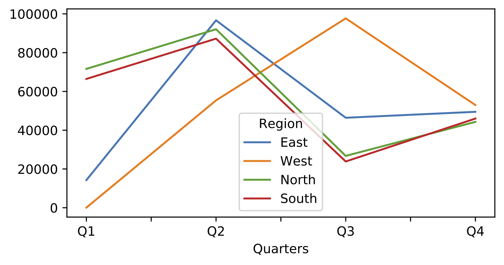
Figure 4-5. Matplotlib plot
Note that in this example, I have used a NumPy array to construct a pandas DataFrame. Providing NumPy arrays allows you to leverage NumPy’s constructors that we met earlier on in this chapter: here we use NumPy to generate a pandas DataFrame based on pseudo-random numbers.
Even if you use the magic command %matplotlib notebook, you can probably notice that Matplotlib was originally designed for static plots rather than for an interactive experience on a web page. That’s why we’re going to use Plotly next, a plotting library designed for the web.
Plotly
Plotly is a JavaScript-based library and can—since version 4.8.0—be used as a pandas plotting backend with great interactivity: You can easily zoom in, click on the legend to select or deselect a category and get a tooltip with info about the data point you’re hovering over. Once you run the following cell, the plotting backend of the whole notebook will be set to Plotly, so if you would rerun the previous chart, it will also be rendered as Plotly chart. For Plotly, you don’t need to run any magic command—setting it as backend is all you need to do:
In[120]:# Set the plotting backend to Plotlypd.options.plotting.backend='plotly'
In[121]:data.plot()
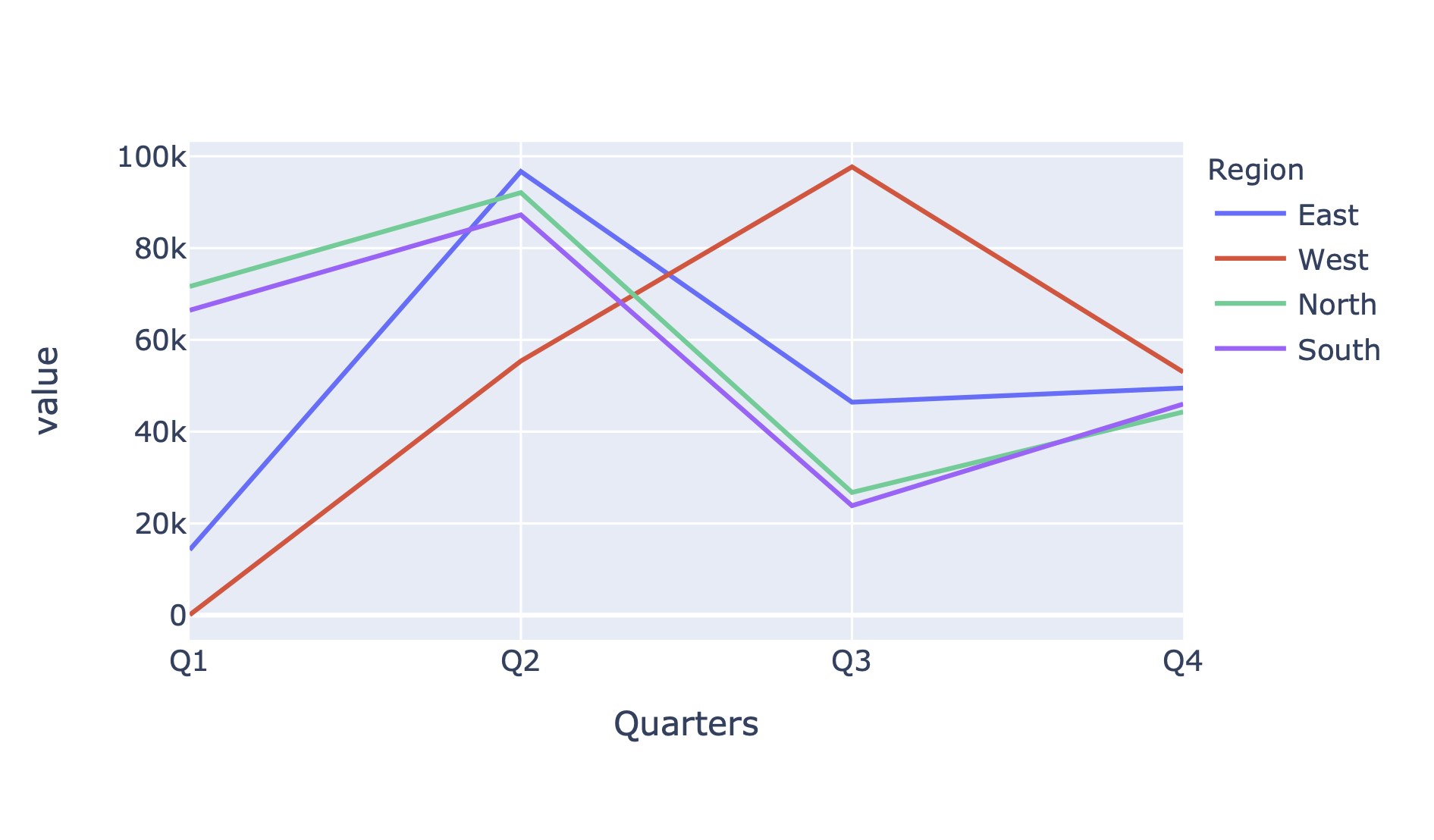
Figure 4-6. Plotly line plot
In[122]:data.plot.bar(barmode='group')
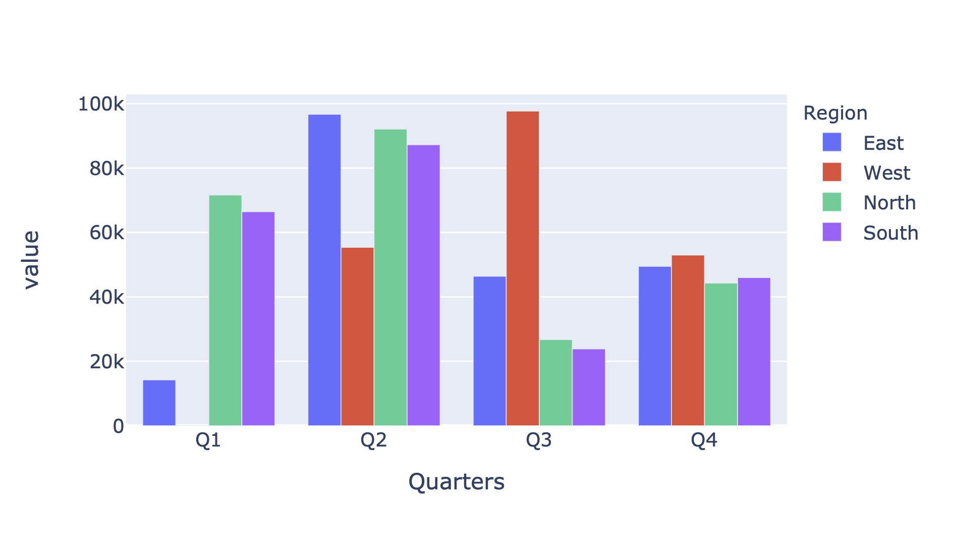
Figure 4-7. Plotly bar plot
Differences in Plotting Backends
If you use Plotly as plotting backend, you’ll need to check the accepted arguments of the plot functions directly on the Plotly docs. For example, you can get an understanding of the barmode=group argument from Plotly’s bar charts documentation.
pandas and the underlying plotting libraries offer a wealth of chart types and options to format the charts in almost any desired way. It’s also possible to arrange multiple plots into a series of subplots. While I don’t have enough space to get into the details here, I will use other plot types during practical examples later in this book. As an overview, Table 4-6 shows the available plot types.
| Type | Description |
|---|---|
|
Line Chart, default when running |
|
Vertical bar chart |
|
Horizontal bar chart |
|
Histogram |
|
Box plot |
|
Density plot, can also be used via |
|
Area chart |
|
Scatter plot |
|
Hexagonal bin plots |
|
Pie chart |
On top of that, pandas offers some higher-level plotting tools and techniques that are made up of multiple individual components. For details, see the pandas visualization documentation. Besides Matplotlib and Plotly, there are many other plotting libraries that you can use with pandas. I’ll present the most popular ones next.
Other Plotting Libraries
The scientific visualization landscape in Python is very active and there are many other high-quality options to choose from that may be the better option for certain use cases:
- Seaborn
-
Seaborn is built on top of Matplotlib. It improves the default style and adds additional plots like heatmaps which often simplify your work: you can create advanced statistical plots with only a few lines of code.
- Bokeh
-
Bokeh is similar to Plotly in technology and functionality: it’s based on JavaScript and therefore also works great for interactive charts in Jupyter notebooks.
- Altair
-
Altair is a library for statistical visualizations based on the Vega project. Altair is also JavaScript-based and offers some interactivity like zooming.
- Holoviews
-
HoloViews is another JavaScript-based package that is focused on making data analysis and visualization easy. With a few lines of code, you can achieve complex statistical plots.
Plotting becomes especially important for bigger datasets that you can’t understand by looking at the raw data anymore. To get our hands dirty with bigger datasets, we need to learn how to load data from external sources—that’s the topic of the next section!
Data Import and Export
So far, we constructed DataFrames from scratch using nested lists, dictionaries or NumPy arrays. This is important to know, but typically, the data is already available and you simply need to read it in and turn it into a DataFrame. To do this, pandas offers a wide range of reader functions. But even if you need to access a proprietary system for which pandas doesn’t offer a built-in reader, you often have a Python package that you can use to connect to that system and from there it’s easy enough to turn the data into a DataFrame. In Excel, data import is the type of work you usually handle via Power Query.
After analyzing and changing your dataset, you might want to push the results back into a database or export it to a CSV file or—given the title of the book—present it in an Excel file to your manager. pandas has various functions to import and export data: table Table 4-7 summarizes just the most important ones.
| Data format/system | Import function | Export function |
|---|---|---|
CSV files |
|
|
JSON |
|
|
HTML |
|
|
Clipboard |
|
|
Excel files |
|
|
SQL Databases |
|
|
As I am going to dedicate the whole next chapter to the topic of reading and writing Excel files, I’ll focus on importing and exporting CSV files in this section, which is one of the most common tasks when analyzing data. We will meet most of the other methods throughout practical examples in the rest of this book.
Importing CSV files
Importing a local CSV file is as easy as providing its path to the read_csv function. MSFT.csv is a CSV file that I downloaded from Yahoo! Finance and it contains the daily historical stock prices for Microsoft—you’ll find it in the companion repository. Since I have stored the CSV file in the same directory as this notebook, I can just provide its name without the need for the full path:
In[123]:msft=pd.read_csv('MSFT.csv')
If you wanted to read the file from a different directory, simply supply the full path to the file, e.g. pd.read_to(r'C:path odesiredlocationmsft.csv).
Use Raw Strings for File Paths on Windows
Since the backslash is used to escape certain characters in a string, you either need to use double backslashes on Windows (C:\path\to\file.csv) or you can prefix the string with an r to turn it into a raw string that interprets the characters literally. This isn’t an issue on macOS or Linux as they use forward slashes in paths.
Often, you will need to supply a few more parameters to read_csv than just the file name. For example, sep allows you to tell pandas what separator or delimiter the CSV file uses in case it isn’t the default comma. We will use a few more parameters in the next section but for the full overview, have a look at the pandas documentation.
Now that we are dealing with big DataFrames with many thousands of rows, typically the first thing is to run the info method to get a summary of the DataFrame. Next, you may want to take a peek at the first and last rows of the DataFrame using the head and tail methods. These methods return 5 rows by default but that can be changed by providing the desired number of rows as argument. You can also run the describe method to get some basic statistics:
In[124]:msft.info()
<class 'pandas.core.frame.DataFrame'>
RangeIndex: 8622 entries, 0 to 8621
Data columns (total 7 columns):
 #   Column     Non-Null Count  Dtype
---  ------     --------------  -----
 0   Date       8622 non-null   object
 1   Open       8622 non-null   float64
 2   High       8622 non-null   float64
 3   Low        8622 non-null   float64
 4   Close      8622 non-null   float64
 5   Adj Close  8622 non-null   float64
 6   Volume     8622 non-null   int64
dtypes: float64(5), int64(1), object(1)
memory usage: 471.6+ KB
In[125]:# I am selecting a few columns because of space issues# You can also just run: msft.head()msft.loc[:,['Date','Adj Close','Volume']].head()
Out[125]:DateAdjCloseVolume01986-03-130.062205103178880011986-03-140.06442730816000021986-03-170.06553713317120031986-03-180.0638716776640041986-03-190.06276047894400
In[126]:msft.loc[:,['Date','Adj Close','Volume']].tail(2)
Out[126]:DateAdjCloseVolume86202020-05-26181.5700073607360086212020-05-27181.80999839492600
In[127]:msft.loc[:,['Adj Close','Volume']].describe()
Out[127]:AdjCloseVolumecount8622.0000008.622000e+03mean24.9219526.030722e+07std31.8380963.877805e+07min0.0577622.304000e+0625%2.2475033.651632e+0750%18.4543135.350380e+0775%25.6992247.397560e+07max187.6633301.031789e+09
The Adj Close stands for adjusted close price and corrects the stock price for corporate actions such as stock splits. Volume is the number of stocks that were traded. The read_csv function also allows you to specify a URL instead of a local CSV file. Since I have included the CSV file in the companion repo, you can also read the data directly from there:
In[128]:# the line break in the URL is only to make it fit on the pageurl=('https://raw.githubusercontent.com/fzumstein/''python-for-excel/master/ch04/MSFT.csv')msft=pd.read_csv(url)
In[129]:msft.loc[:,['Date','Adj Close','Volume']].head(2)
Out[129]:DateAdjCloseVolume01986-03-130.062205103178880011986-03-140.064427308160000
Let’s put this topic on pause for just a moment while we look at how to export data. I will get back to the read_csv function in the next section about time series where we will work with the loaded data. I will also show you some arguments that pd.read_csv accepts.
Exporting CSV files
If you need to pass a DataFrame to a colleague who might not use Python or pandas to work on it, passing the DataFrame as a CSV file is usually a good idea: pretty much every program knows how to import them. To export our sample DataFrame df to a CSV file, you use the to_csv method:
In[130]:df.to_csv('course_participants.csv')
Again, if you’d like to store it in a different location, simply provide the full path. This will produce the file course_participants.csv in the same directory as the notebook with the following content:
user_id,name,age,country,score,continent
1001,Mark,55,Italy,4.5,Europe
1000,John,33,USA,6.7,America
1002,Tim,41,USA,3.9,America
1003,Jenny,12,Germany,9.0,Europe
Now that you know the basics of how to import and export DataFrames via CSV files, you’re ready for the next section where we’ll load stock prices from CSV files to perform time series analysis.
Time Series
A time series is a series of data points along a time-based axis and plays a central role in many different scenarios: While traders use historical stock prices to calculate risk measures, the weather forecast may be based on time series generated by sensors that measure the temperature, humidity and air pressure. The digital marketing department on the other hand often relies on time series generated by web pages, e.g. the source and number of page views per hour, and will use them to draw conclusions with regards to their marketing campaigns.
Time series analysis is one of the main driving forces why data scientists and analysts have started to look for a better alternative to Excel. The following points summarize some of the reasons behind this move:
- Big datasets
-
Time series can quickly grow beyond Excel’s limit of roughly one million rows per sheet. For example, if you work with intraday stock prices on a tick data level, you’re often dealing with hundreds of thousands of records—per stock and day!
- Date and time
-
Excel has various limitations when it comes to handling date and time, the backbone of time series. Missing support for time zones and a number format that is limited to milliseconds are some of them. pandas supports time zones and uses NumPy’s
datetime64[ns]data type which offers a resolution up to nanoseconds. - Missing functionality
-
Excel misses even basic tools to be able to work with time series data in a decent way. For example, if you want to turn a daily time series into a monthly time series, there is no easy way of doing this despite it being a very common task.
DataFrames allow you to work with various time-based indices: DatetimeIndex is the most common one and represents an index with timestamps. Other index types, like PeriodIndex, are based on time intervals such as hours or months. In this section, however, I am going to concentrate exclusively on DatetimeIndex which I will introduce now in more detail.
DatetimeIndex
To construct a DatetimeIndex, pandas offers the date_range function. Most commonly, you use it to generate a certain amount of timestamps with a given frequency. Alternatively, you can give it a start and end timestamp:
In[131]:# This creates a DatetimeIndex based on a start timestamp,# number of periods and frequency ('D' = daily).daily_index=pd.date_range('2020-02-28',periods=4,freq='D')daily_index
Out[131]:DatetimeIndex(['2020-02-28','2020-02-29','2020-03-01','2020-03-02'],dtype='datetime64[ns]',freq='D')
In[132]:# This creates a DatetimeIndex based on start/end timestamp.# The frequency is set to "weekly on Mondays" ('W-MON').weekly_index=pd.date_range('2020-01-01','2020-01-31',freq='W-MON')weekly_index
Out[132]:DatetimeIndex(['2020-01-06','2020-01-13','2020-01-20','2020-01-27'],dtype='datetime64[ns]',freq='W-MON')
In[133]:# Construct a DataFrame based on the weekly_indexpd.DataFrame(data=1,columns=['dummy'],index=weekly_index)
Out[133]:dummy2020-01-0612020-01-1312020-01-2012020-01-271
Let’s now return to the Microsoft stock time series from the last section. When you take a closer look at the column types, you will notice that the Date column has the type Object which means that pandas has interpreted the timestamps as strings:
In[134]:msft=pd.read_csv('MSFT.csv')
In[135]:msft.info()
<class 'pandas.core.frame.DataFrame'>
RangeIndex: 8622 entries, 0 to 8621
Data columns (total 7 columns):
 #   Column     Non-Null Count  Dtype
---  ------     --------------  -----
 0   Date       8622 non-null   object
 1   Open       8622 non-null   float64
 2   High       8622 non-null   float64
 3   Low        8622 non-null   float64
 4   Close      8622 non-null   float64
 5   Adj Close  8622 non-null   float64
 6   Volume     8622 non-null   int64
dtypes: float64(5), int64(1), object(1)
memory usage: 471.6+ KB
There are two ways to fix this and turn it into a datetime data type. The first one is to run the to_datetime function on that column. Make sure to assign the transformed column back to the original DataFrame if you want to change it at the source:
In[136]:msft.loc[:,'Date']=pd.to_datetime(msft['Date'])
In[137]:msft.dtypes
Out[137]:Datedatetime64[ns]Openfloat64Highfloat64Lowfloat64Closefloat64AdjClosefloat64Volumeint64dtype:object
The other possibility is to tell read_csv about the columns that contain timestamps by using the parse_dates argument. parse_dates expects a list of column names or indices. Also, you almost always want to turn timestamps into the index of the DataFrame: this will allow you to look up data easily based on the timestamp. Instead of using the set_index method, you can provide the column via index_col, again as column name or index:
In[138]:msft=pd.read_csv('MSFT.csv',index_col='Date',parse_dates=['Date'])
In[139]:msft.info()
<class 'pandas.core.frame.DataFrame'>
DatetimeIndex: 8622 entries, 1986-03-13 to 2020-05-27
Data columns (total 6 columns):
 #   Column     Non-Null Count  Dtype
---  ------     --------------  -----
 0   Open       8622 non-null   float64
 1   High       8622 non-null   float64
 2   Low        8622 non-null   float64
 3   Close      8622 non-null   float64
 4   Adj Close  8622 non-null   float64
 5   Volume     8622 non-null   int64
dtypes: float64(5), int64(1)
memory usage: 471.5 KB
As info reveals, you are now dealing with a DataFrame that has a DatetimeIndex. If you would need to change another data type, let’s say you wanted Volume to be a float instead of an int, you have again two options: either you provide dtype={'Volume': float} as argument to the read_csv function or you can apply the astype method as follows:
In[140]:msft.loc[:,'Volume']=msft['Volume'].astype('float')msft['Volume'].dtype
Out[140]:dtype('float64')
With time series it’s always a good idea to make sure the index is sorted properly before starting your analysis:
In[141]:msft=msft.sort_index()
And finally, if you need to access only parts of a DatetimeIndex, like the date part without the time, you can do it like so:
In[142]:msft.index.date
Out[142]:array([datetime.date(1986,3,13),datetime.date(1986,3,14),datetime.date(1986,3,17),...,datetime.date(2020,5,22),datetime.date(2020,5,26),datetime.date(2020,5,27)],dtype=object)
Instead of date, you can also use parts of a date like year, month, day etc. To access the same functionality on a regular Series with data type datetime, the syntax is slightly different as you will have to use the dt attribute, e.g. df['column_name'].dt.date. With a sorted DatetimeIndex, we are now ready for some time series fun!
Filtering a DatetimeIndex
Let’s start the fun with a convenience feature: if your DataFrame has a DatetimeIndex, you can easily select rows from a specific time period by using loc with a string in the format YYYY-MM-DD HH:MM:SS. pandas will turn this string into a slice so it covers the whole period. For example, to select all rows from 2019, provide the year as string:
In[143]:msft.loc['2019','Adj Close']
Out[143]:Date2019-01-0299.0991902019-01-0395.4535292019-01-0499.8930052019-01-07100.0204012019-01-08100.745613...2019-12-24156.5153962019-12-26157.7983092019-12-27158.0867312019-12-30156.7242432019-12-31156.833633Name:AdjClose,Length:252,dtype:float64
Let’s take this a step further and plot the data between June 2019 and May 2020:
In[144]:msft.loc['2019-06':'2020-05','Adj Close'].plot()

Figure 4-8. Adjusted close price for MSFT
As usual, you can hover over the Plotly chart to read off the values as tooltip and zoom in by dragging a rectangle with your mouse. Double-click the chart to get back to the default view. Let’s focus on the close price in the next section so I can show you how to work with time zones.
Working with Time Zones
Microsoft is listed at the Nasdaq stock exchange. The Nasdaq is in New York and markets close at 4 PM. To add this additional information to the DataFrame’s index, you can first add the closing hour to the date via DateOffset and then attach the correct time zone to the timestamps via tz_localize. Since this only refers to the close price, we start by selecting a copy of the adjusted close price:
In[145]:msft_tz=msft.loc[:,['Adj Close']].copy()msft_tz.index=msft_tz.index+pd.DateOffset(hours=16)msft_tz.head(2)
Out[145]:AdjCloseDate1986-03-1316:00:000.0622051986-03-1416:00:000.064427
In[146]:msft_tz=msft_tz.tz_localize('America/New_York')msft_tz.head(2)
Out[146]:AdjCloseDate1986-03-1316:00:00-05:000.0622051986-03-1416:00:00-05:000.064427
If you want to convert the timestamps to UTC time zone, use tz_convert. Note that in UTC, the closing hours change depending on whether daylight saving time (DST) was in effect or not:
In[147]:msft_tz=msft_tz.tz_convert('UTC')msft_tz.loc['2020-01-02','Adj Close']# 21:00 without DST
Out[147]:Date2020-01-0221:00:00+00:00159.737595Name:AdjClose,dtype:float64
In[148]:msft_tz.loc['2020-05-01','Adj Close']# 20:00 with DST
Out[148]:Date2020-05-0120:00:00+00:00174.085175Name:AdjClose,dtype:float64
Preparing time series like this will allow you to compare close prices from stock exchanges across different time zones even if the time info is missing or stated in the local time zone. When you analyze stock prices, you are always interested in its performance. Therefore, the next section shows you how to calculate daily returns.
Shifting and Percentage Changes
In finance, the log returns of stocks are often assumed to be normally distributed. By log returns, I mean the natural logarithm of the ratio of the current and previous price. To get a feeling for the distribution of the daily log returns, you can plot a histogram. First, however, you need to calculate the log returns. In Excel, you typically do it with a formula that involves cells from two rows as shown in Figure 4-9.
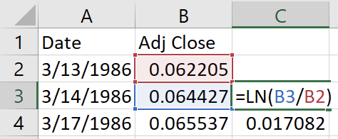
Figure 4-9. Calculating log returns in Excel
Logarithms in Excel and Python
Excel uses LN to denote the natural logarithm and LOG for the logarithm with base 10. Python’s math module and NumPy on the other hand use log for the natural logarithm and log10 for the logarithm with base 10.
With pandas, rather than having a formula accessing two different rows, you use the shift method to shift the values down by one row. This allows you to operate on a single row so your calculations can make use of vectorization. shift accepts a positive or negative integer that shifts the time series down or up by the respective number of rows:
In[149]:msft.iloc[:5,4]
Out[149]:Date1986-03-130.0622051986-03-140.0644271986-03-170.0655371986-03-180.0638711986-03-190.062760Name:AdjClose,dtype:float64
In[150]:msft.iloc[:5,4].shift(1)
Out[150]:Date1986-03-13NaN1986-03-140.0622051986-03-170.0644271986-03-180.0655371986-03-190.063871Name:AdjClose,dtype:float64
You can now write a single vector-based formula that is easy to read and understand. To get the natural logarithm, use NumPy’s log ufunc which is applied to each element:
In[151]:returns=np.log(msft['Adj Close']/msft['Adj Close'].shift(1))returns.head()
Out[151]:Date1986-03-13NaN1986-03-140.0350971986-03-170.0170821986-03-18-0.0257491986-03-19-0.017547Name:AdjClose,dtype:float64
In[152]:returns.plot.hist()
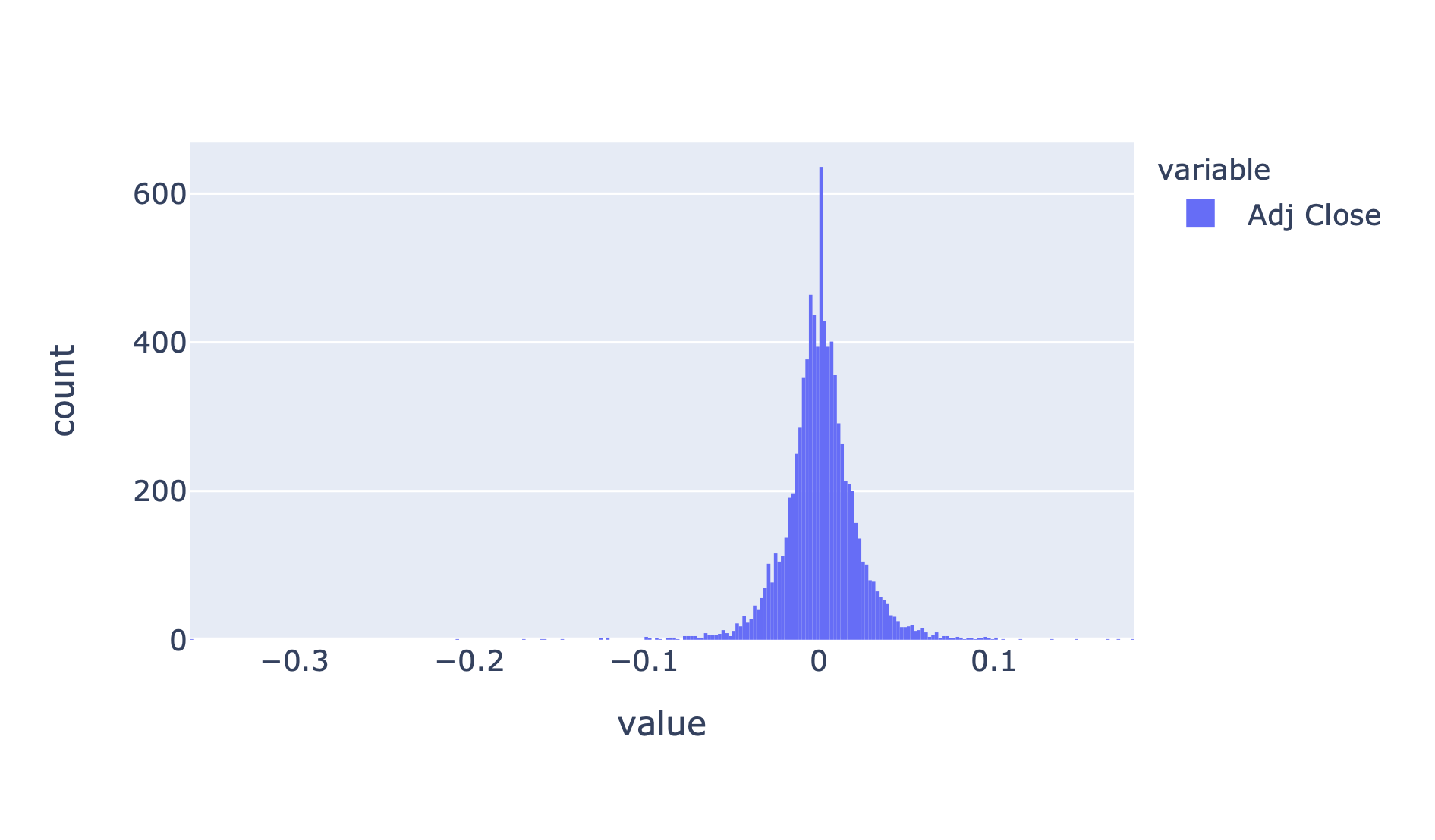
Figure 4-10. Histogram plot
To get simple returns instead, you can use pandas’ built-in pct_change method. By default, it calculates the percentage change from the previous row which is also the definition of simple returns:
In[153]:simple_rets=msft[['Adj Close']].pct_change()simple_rets=simple_rets.rename(columns={'Adj Close':'returns'})simple_rets.head()
Out[153]:returnsDate1986-03-13NaN1986-03-140.0357211986-03-170.0172291986-03-18-0.0254211986-03-19-0.017394
So far, we looked at just the Microsoft stock. In the next section, we’re going to load more time series so we can have a look at other DataFrame methods that require multiple time series.
Rebasing and Correlation
Things get slightly more interesting when we work with more than one time series. Let’s load some additional adjusted close prices for Amazon (AMZN), Google (GOOGL) and Apple (AAPL), also downloaded from Yahoo! Finance:
In[154]:adj_close_parts=[]# list to collect individual DataFramesfortickerin['AAPL','AMZN','GOOGL','MSFT']:# usecols allows us to only read in the Date and Adj Closeadj_close=pd.read_csv(ticker+'.csv',index_col='Date',parse_dates=['Date'],usecols=['Date','Adj Close'])# rename the column into the ticker symboladj_close=adj_close.rename(columns={'Adj Close':ticker})# append the stock's DataFrame to the adj_close_parts listadj_close_parts.append(adj_close)
In[155]:# Combine the 4 DataFrames into a single DataFrameadj_close=pd.concat(adj_close_parts,axis=1)adj_close
Out[155]:AAPLAMZNGOOGLMSFTDate1980-12-120.405683NaNNaNNaN1980-12-150.384517NaNNaNNaN1980-12-160.356296NaNNaNNaN1980-12-170.365115NaNNaNNaN1980-12-180.375698NaNNaNNaN...............2020-05-22318.8900152436.8798831413.239990183.5099952020-05-26316.7300112421.8601071421.369995181.5700072020-05-27318.1099852410.3898931420.280029181.8099982020-05-28318.2500002401.1000981418.239990NaN2020-05-29317.9400022442.3701171433.520020NaN[9950rowsx4columns]
Did you see the power of concat? pandas has automatically aligned the individual time series along the dates. This is why you get NaN values for those stocks that don’t go back as far as Apple. Aligning time series by date is a typical operation that is very cumbersome to do with Excel and therefore also very error-prone. Dropping all rows that contain missing values will make sure that all stocks have the same amount of data points:
In[156]:adj_close=adj_close.dropna()adj_close.info()
<class 'pandas.core.frame.DataFrame'>
DatetimeIndex: 3970 entries, 2004-08-19 to 2020-05-27
Data columns (total 4 columns):
 #   Column  Non-Null Count  Dtype
---  ------  --------------  -----
 0   AAPL    3970 non-null   float64
 1   AMZN    3970 non-null   float64
 2   GOOGL   3970 non-null   float64
 3   MSFT    3970 non-null   float64
dtypes: float64(4)
memory usage: 155.1 KB
Let’s now rebase the prices so that all time series start at 100. This allows us to compare their relative performance in a chart. You can rebase a time series by dividing every value by it’s starting value and multiplying it by 100, the new base. If you did this in Excel, you would typically write a formula with a combination of absolute and relative cell references, then copy the formula for every row and every time series. In pandas, thanks to vectorization and broadcasting, you are dealing with a single formula:
In[157]:# Use a sample from June 2019 - May 2020adj_close_sample=adj_close.loc['2019-06':'2020-05',:]rebased_prices=adj_close_sample/adj_close_sample.iloc[0,:]*100rebased_prices.head(2)
Out[157]:AAPLAMZNGOOGLMSFTDate2019-06-03100.000000100.000000100.00000100.0000002019-06-04103.658406102.178197101.51626102.770372
In[158]:rebased_prices.plot()

Figure 4-11. Rebased time series
To see how independent the different stock returns are from each other you can have a look at their correlations by using the corr method. Unfortunately, pandas doesn’t provide a built-in plot type to visualize the correlation matrix as a heatmap, so we need to use Plotly directly via its plotly.express interface:
In[159]:returns=np.log(adj_close/adj_close.shift(1))returns.corr()
Out[159]:AAPLAMZNGOOGLMSFTAAPL1.0000000.4249100.5034970.486065AMZN0.4249101.0000000.4866900.485725GOOGL0.5034970.4866901.0000000.525645MSFT0.4860650.4857250.5256451.000000
In[160]:importplotly.expressaspxfig=px.imshow(returns.corr(),x=adj_close.columns,y=adj_close.columns,color_continuous_scale=list(reversed(px.colors.sequential.RdBu)),zmin=-1,zmax=1)fig.show()
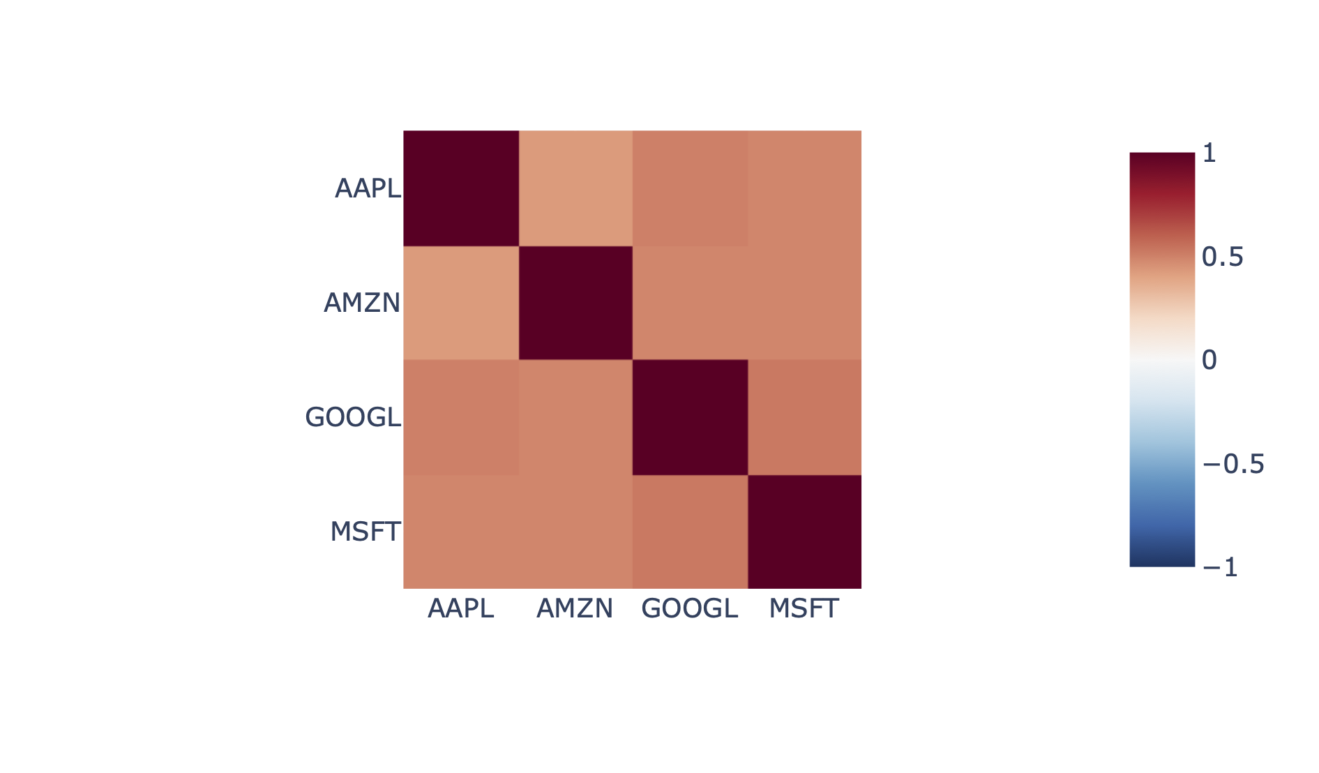
Figure 4-12. Correlation heatmap
If you want to understand how imshow works in detail, you can have a look at the Plotly Express API docs. At this point, we have already learned quite a few things about time series including how to combine and clean them and how to calculate returns and correlations. But what if you decide that daily returns are not a good base for your analysis but you prefer monthly returns? How you can change the frequency of time series data is the topic of the next section.
Resampling
A regular task with time series is up- and downsampling. Upsampling means that the time series is converted into one with a higher frequency and downsampling means that it is converted into one with a lower frequency. On financial factsheets, you often show monthly or quarterly performance, for example. To turn the daily time series into a monthly one, use the resample method that accepts a frequency string like M for end-of-calendar-month or BM for end-of-business-month. You can find a list of all frequency strings in the pandas docs. Similar to how groupby works, you then chain a method that defines how you are resampling. I am using last to always take the last observation of that month:
In[161]:end_of_month=adj_close.resample('M').last()end_of_month.head()
Out[161]:AAPLAMZNGOOGLMSFTDate2004-08-312.13270838.13999951.23623717.6736302004-09-302.39612740.86000164.86486817.9002152004-10-313.24018234.13000195.41541318.1073742004-11-304.14607239.68000091.08107819.3444212004-12-313.98220744.29000196.49149319.279480
Instead of last, you can choose any other method that works on groupby, like sum or mean. There is also ohlc, which conveniently returns the open, high, low and close value over that period. This may serve as the source to create the typical candlestick charts that are often used with stock prices.
If that end-of-month time series would be all you have and you need to produce a weekly time series out of it, you can upsample your time series. By using asfreq, you are telling pandas not to apply any transformation and hence you will see most of the values showing NaN. If instead, you wanted to forward-fill the last known value, use the ffill method:
In[162]:end_of_month.resample('D').asfreq().head()# no transformation
Out[162]:AAPLAMZNGOOGLMSFTDate2004-08-312.13270838.13999951.23623717.673632004-09-01NaNNaNNaNNaN2004-09-02NaNNaNNaNNaN2004-09-03NaNNaNNaNNaN2004-09-04NaNNaNNaNNaN
In[163]:end_of_month.resample('W-FRI').ffill().head()# forward fill
Out[163]:AAPLAMZNGOOGLMSFTDate2004-09-032.13270838.13999951.23623717.6736302004-09-102.13270838.13999951.23623717.6736302004-09-172.13270838.13999951.23623717.6736302004-09-242.13270838.13999951.23623717.6736302004-10-012.39612740.86000164.86486817.900215
Downsampling data is one way of smoothing a time series. Calculating statistics over a rolling window is another way: the next section has the details.
Rolling Windows
When you calculate time series statistics, you often want a rolling statistic such as the moving average: the moving average takes a subset of the time series, let’s say 25 days, and takes the mean from this subset before moving the window forward by one day. This will result in a new time series that is smoother and less prone to outliers. If you are into algorithmic trading, you may be looking at the intersection of the moving average with the stock price and take this (or some variation of it) as a trading signal. pandas offers the rolling method which accepts the number of observations as argument. You then chain it with the statistical method that you want to use—in the case of the moving average it’s the mean:
In[164]:# Plot the moving average for MSFT with data from 2019msft19=msft.loc['2019',['Adj Close']].copy()# Add the 25 day moving average as a new column to the DataFramemsft19['25day average']=msft19['Adj Close'].rolling(25).mean()msft19.plot()
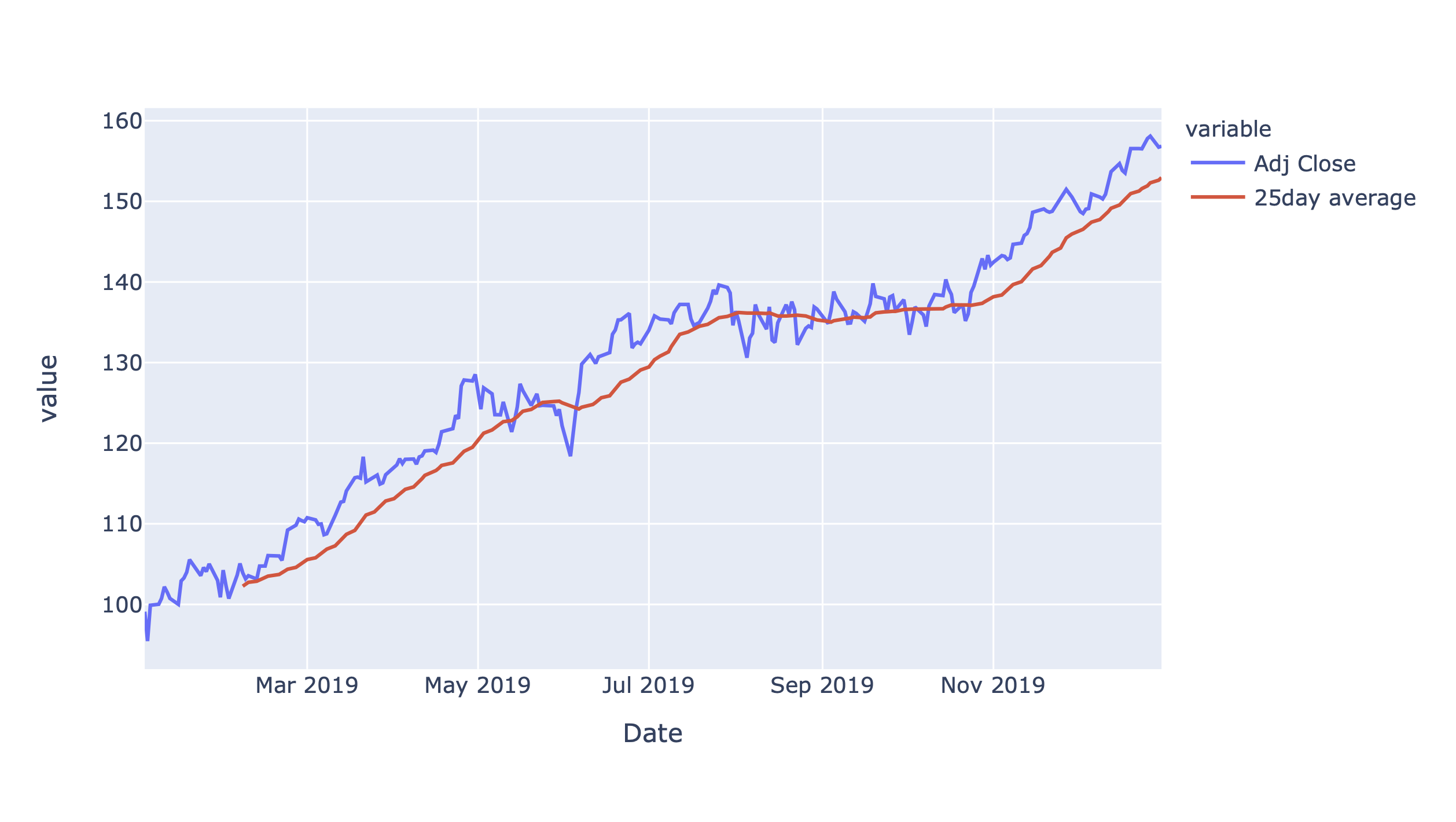
Figure 4-13. Moving average plot
Instead of mean, you can use many other statistical measures including count, sum, median, min, max, std or var (std stands for standard deviation and var for variance). Or you can use your own function via apply(your_function).
I have now shown you the most important functionality of pandas. It’s equally important though to understand where pandas has its limits, even though they may still be far away right now.
Limitations with pandas
When your DataFrames start to get bigger, you definitely want to know the upper limit of what a DataFrame can hold. Unlike Excel, where you have a hard limit of roughly one million rows and 12,000 columns per sheet, pandas only has a soft limit: all data must fit into the available memory of your machine. If that’s not the case, there might be some easy fixes: for example, you can load only those columns from your dataset that you need or you may be able to delete intermediate results to free up some memory. If that doesn’t help, there are quite a few projects that will feel familiar to pandas users but work with big data. One of the projects, Dask, works on top of NumPy and pandas and allows you to work with with big data by splitting it up into multiple pandas DataFrames behind the scenes. Dask also parallelizes computations by taking advantage of multi-core CPUs, thereby making certain calculations faster with large datasets. Other big data projects that work with some sort of DataFrame are Modin, Koalas, Vaex, PySpark, cuDF, Ibis or PyArrow. We will briefly touch on Modin in the next chapter but other than that, this is not something we are going to explore further since the datasets we use in this book are of moderate size.
Conclusion
This chapter was packed with new concepts and tools to analyze datasets in pandas. We learned about data acquisition and data cleaning, including how to load data, extract subsets and how to deal with missing or duplicate data. We also covered how to analyze data by combining and aggregating it, calculating descriptive statistics and presenting the results with plots. While it may take a while to digest everything, it probably won’t take long before you will understand the immense power you are gaining by adding pandas to your tool belt. If you are using Excel for time series analysis, I would strongly recommend you to play around with pandas rather sooner than later, as this is the area where I feel Excel has fallen behind the most. For example, being able to write a single formula to get the percentage change out of a DataFrame with hundreds of time series is not just easier but also a lot less error-prone than if you have to copy a formula in Excel for every time series and every single data row.
Knowing how to use pandas doesn’t mean you have to get rid of Excel though, as the two worlds can play very nicely together: pandas DataFrames are a great way to transfer data from one world to the other as we will see in the remaining chapters. To start this journey, the next chapter will show you how pandas—in combination with various Excel reader and writer libraries—can be used to automate tedious manual processes like the aggregation of Excel files into summary reports.