
Chapter 2. Development Environment
After seeing a few lines of code in the last chapter, you probably can’t wait to learn the basics of Python. However, to learn Python, you first need to set up your computer to be able to write and run Python code. As a VBA developer, you could simply type Alt-F11 in Excel to open the VBA editor where you could write and run your code. With Python, it’s a bit more work.
This chapter introduces you to the three tools that we will work with throughout this book: the command line, Jupyter notebooks and Visual Studio Code (VS Code). We will start with a quick introduction to the command line before we install Python via the Anaconda distribution. We then play around with Jupyter notebooks before introducing VS Code, a powerful text editor. Figure 2-1 shows an overview of the tools that will be introduced in this chapter.

Figure 2-1. Development environment
You’ll use the command line mainly to run Python code and start Jupyter notebooks. Jupyter notebooks run in your web browser and allow you to experiment with your first lines of Python code in a beginner-friendly and visually attractive way. Jupyter notebooks come with Anaconda as part of the pre-installed packages. Like Excel, they allow you to work with data and charts which makes them an interesting competitor to Excel files in certain work environments. VS Code is a text editor that allows you to write and run Python scripts easily. It works great for managing slightly more complex projects that don’t fit into a single Jupyter notebook. On top of that, VS Code allows you to run Jupyter notebooks without having to use your web browser. It also gives you access to an integrated command line.
As this book is about Excel, I am concentrating on detailed instructions for Windows and macOS. However, everything in [Link to Come] runs on Linux, too. Let’s start this chapter by introducing our first tool: the command line!
Command Line
The command line is one of the most important tools to master when you start programming: it allows you to run your code, install a Python package or run an interactive Python session. The command line is already available on your system—no need to install anything. However, before I show you how to use it in this section, let’s first make sure that your operating system shows file extensions in your folders. This way, the file names will look the same on the command line as they do in the File Explorer on Windows or Finder on macOS which helps you avoid the sort of confusion I’ll point out in the opening sample of the next section.
File Extensions
A desperate client once asked me why their code wasn’t working. When I took a look at the involved Excel file, it was immediately clear what was going on: the file was called test.xlsx.xlsx. An error that is easy to spot—if you have configured your operating system to show file extensions. When working with Excel, showing file extensions also helps you to understand whether you’re dealing with the default xlsx file, a macro-enabled xlsm file or any of the other Excel file formats. Additionally, you will always refer to your Excel files with their extension in your Python code, which is why I highly recommend you to show them so your files show up as myfile.xlsx or myfile.py rather than as myfile. Unfortunately, Windows and macOS hide file extensions by default, so here is how to change that:
- Windows
-
Open a File Explorer and click on the
Viewtab. Under theShow/Hidegroup, activate the checkboxFile name extensions. - macOS
-
Open the Finder and go to
Preferencesby typingCommand-,. Under theAdvancedtab, check the boxShow all filename extensions.
Now that your file names show up with their extensions, let’s learn the most important commands that we will use on the command line!
Running Commands
The most basic tool to run Python code is the command line. I will use this name throughout the book to mean the Command Prompt or Anaconda Prompt on Windows and the Terminal on macOS. I will introduce the Anaconda Prompt in the next section. The command line comes in handy for finding the root cause of seemingly obscure errors: if, for example, you run your Python code with VS Code, certain settings may make your code behave differently from what you would expect. Being able to fall back to a clean command line can often confirm if there’s something wrong with your code or with the way you run it. The command line is also how you interact with a Linux server where you would typically run the Python scripts that we are writing in [Link to Come]: for example, a server can run your scripts every hour to automate tedious tasks involving Excel files—more about that in Chapter 5.
If you are new to the command line, don’t worry: with just a handful of commands you’re gaining a lot of power already. Once you get used to it, the command line is often faster and more convenient than clicking your way through graphical user menus. Let’s get started:
- Windows
-
Click on the Start menu button (the Windows icon in the bottom left corner), then start typing
command(there is no field to type into, just start typing when the Start menu is shown). You should see the entryCommand Promptappear. If it is selected, hitEnteror use your mouse to click on it. If you prefer to open it from the Start menu folders, you will find the Command Prompt under the folderWindows System. Once the Command Prompt appears, it will look something like this, ready to accept your commands:C:Usersfelix>
- macOS
-
Press
Command-Space baror open the Launchpad, then type inTerminaland hitEnter. Alternatively, you can open the Finder and navigate toApplications>Utilitieswhere you will find the Terminal app that you can double-click. Once the Terminal appears, it will look something like this, ready to accept your commands:felix@MacBook-Pro ~ %
If you are on an older Mac, it looks rather like this:
MacBook-Pro:~ felix$
To see the full path of the current directory, type
pwdfollowed byEnter.pwdstands for print working directory. On macOS and other Unix-like systems,~stands for the home directory. The full home directory on macOS is usually/Users/username.
Having either the Command Prompt or Terminal up and running, try out the commands outlined in Table 2-1. Each command is explained in more detail following the table.
Hit Enter to Confirm Commands
To make the command line do something, you always need to hit Enter after typing in a command. While I mention this with the following few commands, the rest of this book will not explicitly mention this anymore.
| Command | Windows | macOS |
|---|---|---|
List files in current directory |
|
|
Change directory (relative) |
|
|
Change directory (absolute) |
|
|
Change to D drive |
|
(doesn’t exist) |
Change to parent directory |
|
|
Command history |
|
|
- List files in current directory
-
On Windows, type in
dir, then hitEnter: This will print the content of the directory you are currently in.On macOS, type in
ls -lafollowed byEnter(-lawill format the output as list and include all files, including hidden ones).While
dirstands for directory,lsstands for list. - Change directory
-
Type
cd Downand hit thetabkey. If you are in your home folder, the command line should most likely be able to autocomplete it tocd Downloads. If you are in a different folder or don’t have a folder calledDownloads, simply start to type the beginning of one of the directory names you saw in the previous command before hittingtabto autocomplete. Then change into the Downloads directory by hittingEnter. If you’d like to change into a directory that is not a subdirectory of your current directory, you will need to type in the full absolute path.cdstands for change directory. If you are on Windows and need to change your drive, you first need to type in the drive name before you can change into the correct directory:C:Usersfelix> D: D:> cd data D:data>
Note that by starting your path with a directory or file name that is within your current directory, you are using a relative path, e.g.
cd Downloads. If you would like to go to a directory somewhere else, you can type in an absolute path, e.g.cd C:Userson Windows orcd /Userson macOS (mind the forward slash at the beginning). - Change to parent directory
-
To go to your parent directory, i.e. one level up in your directory hierarchy, type
cd ..followed byEnter. You can combine this with a directory name, e.g. if you want to go up one level, then change to theDesktop, do:cd ..Desktop. On macOS, replace the backslash with a forward slash. - Command history
-
Hit the
up arrowkey to scroll through the previous commands. This will save you a lot of keystrokes if you need to run the same commands over and over again. If you scroll too far, use thedown arrowkey to scroll back.
And that’s already it! You are now able to fire up a command line and run commands in the desired directory. You’ll be using this right away to fire up an interactive Python interpreter. First, we need to install Python though—we’ll do this via the Anaconda distribution, as I will show you next.
The Anaconda Python Distribution
Anaconda is arguably the most popular Python distribution used for data science and comes with hundreds of third-party packages preinstalled: it includes Jupyter notebooks and most of the other packages like pandas and xlwings, that this book will use extensively. Anaconda is free and guarantees that all the included packages are compatible with each other. It installs into a single folder and can easily be uninstalled again. Let’s get started by downloading and installing Anaconda.
Installation
Go to the Anaconda homepage and download the latest version of the Anaconda installer (Individual Edition). Make sure to download the 64-bit graphical installer for the Python 3.x version1. Once downloaded, double-click the installer to start the installation process. You can change the installation path if you want, but otherwise, make sure to accept all the defaults. For more detailed installation instructions, you can follow the official documentation that is accessible from the Anaconda homepage.
Other Python Distributions
While this book assumes that you have the Anaconda Individual Edition installed, the code and concepts shown will work with any other Python installation, too. There is only one distribution that I would avoid: the Python installation from the Windows store as it doesn’t have full access to all directories.
With Anaconda installed, it’s now time to test if it was correctly installed—most importantly if we can launch a Python interpreter!
Anaconda Prompt
First, let’s introduce a little twist to the command line: on Windows, you need to switch from the normal Command Prompt to the Anaconda Prompt. This will automatically activate the Conda environment with the name base as shown by (base) at the beginning of your input line. I’ll say more about this under “Conda Environments” but for the time being, just remember that from now on you always want your command line to show (base) in order for everything to work properly. In more detail:
- Windows
-
Click on the Start menu button and start typing
Anaconda Prompt. You should see the entryAnaconda Promptappear. Choose theAnaconda Prompt, not theAnaconda Powershell Prompt. If it is selected, hitEnteror use your mouse to click on it. If you prefer to open it from the Start menu folders, you will find it under theAnaconda3folder. It is a good idea to pin the Anaconda Prompt to your taskbar as you will use it regularly throughout this book. Once the Anaconda Prompt appears, it will start with(base):(base) C:Usersfelix>
Command Line on Windows
From here on, when I write Command Line, on Windows I refer to the Anaconda Prompt. The Anaconda Prompt is nothing else than a standard Command Prompt that automatically activates the base Conda environment.
- macOS
-
On macOS, everything should work out of the box with the Terminal after installing Anaconda. However, if you had it running during the Anaconda installation, right-click on the Terminal in the dock and select
Quitor hitCommand-Q. Then start the Terminal again. Note that clicking on the red cross on the top left of the Terminal window will not quit it. If the Terminal shows(base)at the beginning of a new line, you are all set:(base) felix@MacBook-Pro ~ %
With the command line showing properly showing (base), it’s about time to make contact with Python: in the next section, I’ll show you how to run an interactive Python session.
Python REPL: An Interactive Python Session
You can start an interactive Python session by running the python command:
(base) C:Usersfelix>python
Python 3.8.3 (default, Jul 2 2020, 17:30:36) [...] :: Anaconda, Inc. on win32
Type "help", "copyright", "credits" or "license" for more information.
>>>
The text that gets printed in a Terminal on macOS will slightly differ, but otherwise, it works the same. While this book is based on Python 3.8, all samples should work unchanged with newer versions of Python, too.
Command Line Notation
Going forward I will start lines of code with $ to denote that they are typed into either the Anaconda Prompt on Windows or the Terminal on macOS with the base environment activated. For example, to launch an interactive Python interpreter on the command line I will write:
$ python
which on Windows will look similar to this:
(base) C:Usersfelix>python
and on macOS similar to this:
(base) felix@MacBook-Pro ~ % python
Let’s play around a bit! Note that >>> in an interactive session means that Python expects your input, you don’t have to type this in. Follow along by typing in each line that starts with >>>, confirming with the Enter key:
>>> 3 + 4
7
>>> "python " * 3
'python python python '
This interactive Python session is also referred to as Python REPL which stands for read-eval-print loop: Python reads your input, evaluates it and prints the result instantly while waiting for your next input. Remember the Zen of Python that I mentioned in the previous chapter? You can now read the full version to get some insight into the guiding principles of Python (smile included). Simply run this line:
>>> import this
To exit out of your Python session, type quit() followed by the Enter key. Alternatively, type Ctrl-Z on Windows, then hit the Enter key. On macOS, simply hit Ctrl-D, no need to hit Enter.
Having exited out again of the Python REPL, it’s a good moment to play around with conda, Anaconda’s package manager.
Package Managers: Conda and pip
I already said a few words about pip, Python’s package manager in Chapter 1: pip takes care of downloading, installing, updating and uninstalling Python packages as well as their dependencies and sub-dependencies. While Anaconda works with pip, it has a built-in alternative package manager called Conda. As a short recap: packages add additional functionality to your Python installation that is not covered by the standard library. pandas, which I will properly introduce in Chapter 4, is an example of such a package. Since it comes preinstalled in Anaconda’s Python installation, you don’t have to install it manually though.
Conda vs. pip
With Anaconda, it’s best to first install everything you can via conda and only use pip to install those packages that are not available via conda. Otherwise, you may run the risk that conda overwrites packages that were previously installed with pip.
Whenever this book requires a package that is not included in the Anaconda installation, I will point this out explicitly and show you how to install it. Table 2-2 gives you an overview of the commands that you will use most often for both package managers, to be typed on a command line. These commands will allow you to install, update and uninstall your third-party packages.
| Action | Conda | pip |
|---|---|---|
List all installed packages |
|
|
Install the latest version |
|
|
Install a specific version |
|
|
Update a package |
|
|
Uninstall a package |
|
|
For example, to see what packages are already available in your Anaconda distribution, type:
$ conda list
For a more comprehensive overview of the commands of both package managers, simply type conda or pip on your command line which will print all available commands.
You know now how to start a Python interpreter and how to use the package managers. In the next section, I’ll explain what the (base) at the beginning of your command line actually means.
Conda Environments
You may have been wondering what the meaning of (base) is that the command line shows after the installation of Anaconda. It is the name of the active Conda environment. A Conda environment is a separate “Python world” with a specific version of Python and a set of installed packages with specific versions. Why is this necessary? When you start to work on different projects in parallel, they will have different requirements: one project may use Python 3.8 with pandas 0.25.0 while another project may use Python 3.9 with pandas 1.0.0. Code that is written for pandas 0.25.0 will often require changes to run on pandas 1.0.0 so you can’t just upgrade your Python and pandas versions without making changes to your code. Using a Conda environment for each project makes sure that every project runs with the correct dependencies. While Conda environments are specific to the Anaconda distribution, the concept exists with every Python installation under the name virtual environment. Conda environments are more powerful though as they make it easier to deal with different versions of Python itself, not just packages.
While you work through this book, you will not have to change your Conda environment as we’ll always be using the default base environment. However, when you start building real projects, it’s good practice to use one Conda or virtual environment for each project to avoid any potential conflicts between their dependencies. Everything you need to know about dealing with multiple Conda environments is explained in Appendix A.
Having resolved the mystery around Conda environments, it’s time to introduce the next tool, one that we will use very intensively during the remainder of this chapter: Jupyter notebooks!
Jupyter Notebooks
In the previous section, I showed you how to run an interactive Python session on the command line. This is sometimes useful if you want a bare-bones environment to test out something simple. For the majority of your work, however, you want an environment that is easier to use. For example, going back to previous commands and displaying charts is hard with a Python REPL running on the command line. Fortunately for us, Anaconda comes with much more than just the Python interpreter: it also includes Jupyter notebooks which have emerged as one of the most popular ways to run Python code in a data science context.
Jupyter notebooks allow you to tell a story by combining executable Python code with formatted text, pictures and charts into an interactive notebook that runs in your browser. They are very beginner-friendly and thus especially useful for the first steps of your Python journey. They are, however, also hugely popular for prototyping and researching as others can easily reproduce the research. Consequently, I will present the majority of code samples in this book in the style of a Jupyter notebook. Jupyter notebooks have become a big competitor to Excel workbooks as they cover roughly the same use case: you can quickly prepare, analyze and visualize data. The difference to Excel is that all of it happens by writing Python code instead of clicking around to select a cell range or to change the color in a chart. Having Python code visible in your notebook makes it easy to see what’s going on as the code is not hidden away behind the cell value like in Excel. Another advantage of Jupyter notebooks is that they are easy to run either locally or on a remote server. Running a program on a server means that you can automate it, something that is hard to do with Excel alone. Jupyter notebooks can be used to run code in many different programming languages, but in this book I am only using them to run Python. Before saying anything else, let’s give it a try!
A First Notebook
On your command line, launch a Jupyter notebook server in your practice directory:
$ cd C:Usersusernamepython-for-excel
$ jupyter notebook
This will automatically open your browser and show the files in the directory from where you were running the command. If Jupyter doesn’t manage to open the browser automatically, follow the instructions that are printed on the command line to open the web page manually. On the top right of the Jupyter landing page, click on New, then select Python3 from the dropdown list. This will open a new browser tab with your first empty Jupyter notebook as shown in Figure 2-2.

Figure 2-2. An empty Jupyter notebook
Click on Untitled1 next to the Jupyter logo to rename your workbook into first_notebook. When you change to the browser tab with the Jupyter landing page, you will see your notebook there as first_notebook.ipynb. The file extension ipynb comes from the fact that Jupyter notebooks were originally called IPython notebooks. What you see on the screen is called a cell—the next section introduces them in more details!
Notebook Cells
Let’s go back to the browser tab with the notebook: In Figure 2-2 you can see an empty cell with a blinking cursor. If the cursor doesn’t blink, click into the cell with your mouse, i.e. to the right of In [ ]. Now repeat the exercise from the last section: type in 3 + 4 and run the cell by either clicking on the Run button in the menu bar at the top or—much easier—by hitting Shift-Enter. This will run the code in the cell, print the result below the cell and jump to the next cell. In this case, it inserts an empty cell below as we only have one cell so far.
Cell Output
If the last line in a cell returns a value other than None, it is automatically printed by the Jupyter notebook under Out [ ]. I will explain None in Chapter 3. However, not all output in Jupyter notebooks is shown as Out [ ] cell. When you use the print function or when you get an exception, it is printed directly below the In cell. Since the code samples in this book reflect the behavior of Jupyter notebooks, you will accordingly not see the Out cell for these types of outputs.
While a cell is calculating, it shows In [*] and when it’s done it gets a number assigned, e.g. In [1]. Below the cell you will have the corresponding output labeled with the same number: Out [1]. Every time you run or re-run a cell, the counter increases. Going forward, I will show everything that you can easily run in a Jupyter notebook cell in this format, e.g. for the calculation from before:
In[1]:3+4
Out[1]:7
This allows you to follow along easily by typing the input line 3 + 4 into a notebook cell. When running it by hitting Shift-Enter, you will get what I show as output under Out[1]. If you read this book in an electronic format supporting colors, you will notice that strings, numbers etc. are formatted differently to make it easier to read: this is called syntax highlighting. Cells can have different types, two of which are of interest to us:
- Code
-
This is the default type. Use it whenever you want to run Python code.
- Markdown
-
Markdown allows you to use standard text characters for formatting. It can, therefore, be used to include nicely formatted explanations and instructions in your notebook.
To change a cell’s type to Markdown, select the cell, then choose Markdown in the dropdown at the top of the notebook where it currently shows Code. I’ll show you a keyboard shortcut to switch back and forth in a moment. After changing an empty cell into a Markdown cell, type in the following text which explains the most important Markdown rules:
# This is a first level title

## This is a second level title

Normal text doesn't require any special treatment.

Bullet points:

* An item
* Another item

You can also make your text *italic* or **bold** or `monospaced`.

Equations can be included via LaTeX syntax: $ e ^{ipi} + 1 = 0 $

Code that isn't supposed to be executed can be included like this:

```python
print("hello world!")
```
After hitting Shift-Enter, the text will be rendered into nicely formatted HTML. To include a picture, type this in a new Markdown cell:

The picture python.png needs to be a file path or a URL. In this sample, it expects the picture in the same directory as your notebook. If it would be in a directory called images, you would use . If you need a bit more control you can also use HTML notation that allows you to set some attributes, for example (still in a Markdown cell):
<img src="python.png" width="100">
At this point, your notebook should look like in Figure 2-3.
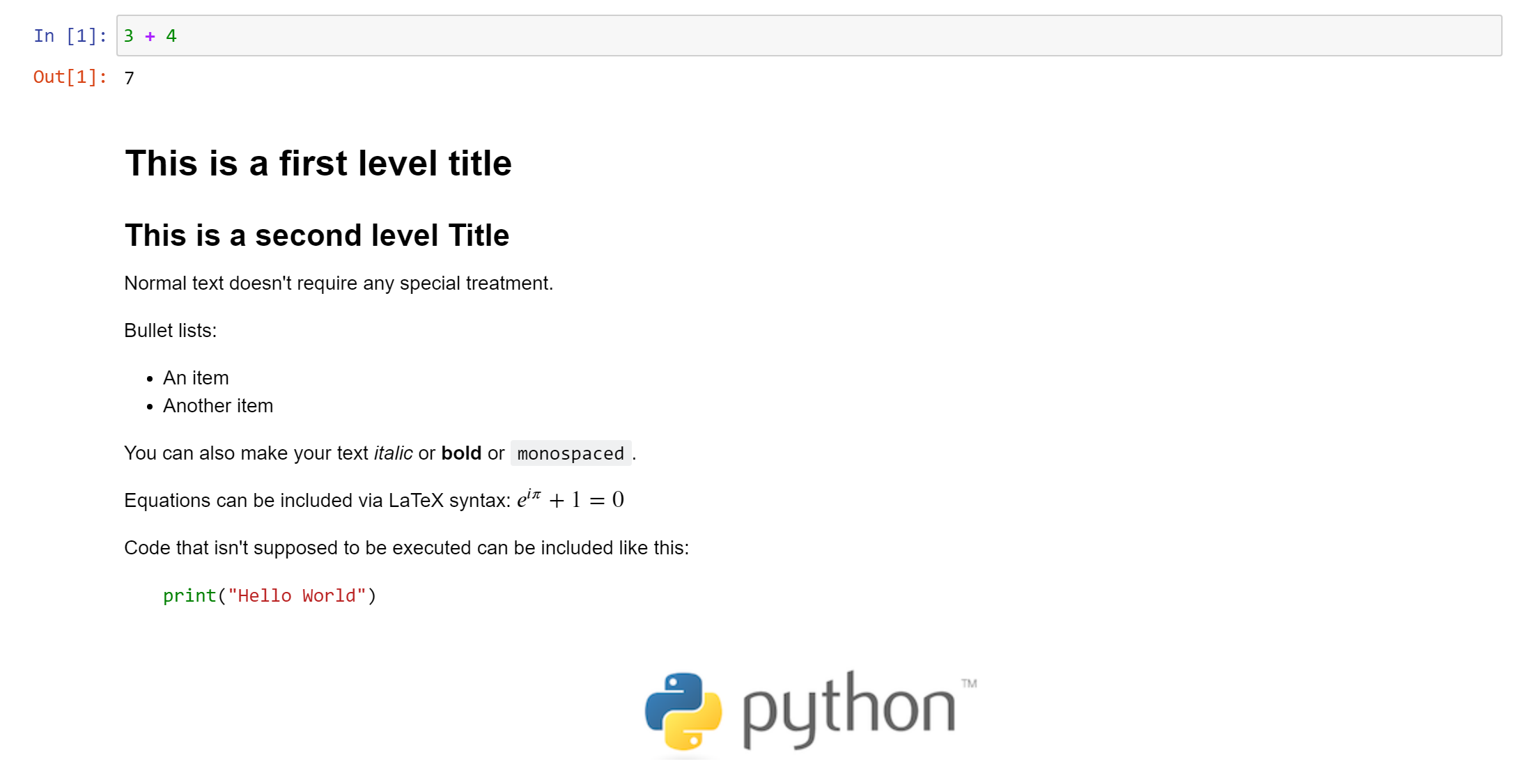
Figure 2-3. The notebook after running a few cells
This section introduced you to the code and markdown cell types. To interact with cells, you have two different modes, which I will explain in the next section.
Edit vs. Command Mode
There are two modes of how to interact with notebook cells:
- Edit mode
-
When you click into a cell, the border around the selected cell turns green and the cursor in the cell starts blinking. Instead of clicking into a cell, you can also hit
Enterwith the cell selected that you want to edit. Hit theEsckey to switch out of edit mode into command mode. - Command mode
-
When you are in command mode, the border around the selected cell will be blue and there is no cursor blinking. To switch into command mode, hit the
Esckey. The most important keyboard shortcuts, which you can use while you are in command mode, are shown in Table 2-3.
| Shortcut | Effect |
|---|---|
|
Run the cell (works also in edit mode) |
|
Move cell selector up |
|
Move cell selector down |
|
insert a new cell below the current cell |
|
insert a new cell above the current cell |
|
delete the current cell (type two times the letter |
|
change cell type to Markdown |
|
change cell type to code |
Knowing these few keyboard shortcuts will allow you to work with notebooks very efficiently without having to switch to the mouse all the time. In the next section, I’ll show you another great feature that can make your life easier: magic commands.
Magic Commands
Magic commands are a set of simple commands which cause a cell to behave in a certain way or make cumbersome tasks so easy that it almost feels like magic. You write magic commands in cells like Python code but they either start with %% or %: commands that affect the whole cell start with %% while commands that only affect a single line start with %. For example, if you want to check how long it takes to run a certain cell, start your cell with %%time:
In[2]:%%timen=1000000sum(range(n))
CPU times: user 17.8 ms, sys: 97 µs, total: 17.9 ms
Wall time: 17.8 ms
Out[2]:499999500000
If you are interested in only a single line of code, you can use:
In[3]:%timen=1000000sum(range(n))
CPU times: user 1e+03 ns, sys: 0 ns, total: 1e+03 ns
Wall time: 4.05 µs
Out[3]:499999500000
Wall time vs. CPU times
Measuring how long it takes to run a cell can be useful for simple performance tuning as you can easily compare two cells with different code snippets. Wall time is the elapsed time from the start to the end of the program, i.e. in this case the cell or a single line. CPU times measures the time spent on the CPU which can be lower if the program has to wait for the CPU to become available or higher if the program is running on multiple CPU cores in parallel. On Windows, you will only be able to see the wall time. To measure the time more accurately, use %timeit instead of %time which runs the cell multiple times and takes the average of all runs.
To list all currently available magic functions, you can run %lsmagic and for a detailed description run %magic. For example, the magic command %pwd stands for print working directory:
In[4]:%pwd
Out[4]:'/Users/felix/python-for-excel/ch02'
Now that you know all the basics of how to work with a Jupyter notebook, the next section moves on by showing you a common trap to watch out for.
Run Order Matters
As easy and user-friendly notebooks are to get started, they also make it easy to get into potentially confusing states when cells are not run sequentially. Assume you have the following notebook cells that are run from top to bottom:
In[5]:a=1In[6]:aOut[6]:1In[7]:a=2
Cell Out[6] prints the value 1 as expected. However, if you now go back and run In[6] again, you will end up in this situation:
In[5]:a=1
In[8]:a
Out[8]:2
In[7]:a=2
Now, a has the value 2 in Out[8] which is clearly not what you will expect, especially if cell In[7] is further away. To prevent such cases, it is good practice to re-run not just a single cell, but all of its previous cells, too. Jupyter notebooks offer you an easy way to accomplish this under the menu Cell > Run all above. You won’t run into this issue with standard Python files as they are always executed from top to bottom.
After these words of caution, let’s see how you can shut down your notebook again!
Shutting Down a Notebook
Every notebook runs in a separate Jupyter kernel. A kernel is the “engine” that runs the Python code you type into a notebook cell. Every kernel uses resources from your operating system in the form of CPU and RAM. Therefore, when you close a notebook, you should also shut down its kernel so that the resources can be used again by other tasks which prevents your system from slowing down. The easiest way to accomplish this is by closing a notebook via File > Close and Halt. If you just close the browser tab, the kernel will not be shut down automatically. Alternatively, on the Jupyter landing page, you can close running notebooks from the tab Running.
To shut down the whole Jupyter server, click on Quit on the Jupyter landing page. If you have already closed your browser, you can type Ctrl-C twice on the command line where the notebook server is running or close the command line altogether.
You don’t always have to start the notebook server, run cells in your browser manually and shut it down again. You can also run a notebook in a non-interactive mode. How this works is the topic of the next section.
Jupyter CLI
You used the Jupyter CLI for the first time when you were running the jupyter notebook command. CLI stands for command line interface and means any sort of program that runs on the command line. Apart from spinning up a Jupyter notebook server, the Jupyter CLI has a few more tricks up its sleeve. In this section we’re going to look at two of them: we’ll start by learning how to run a notebook from the command line before exporting a Jupyter notebook as a static HTML page.
Run a notebook from the command line
If you want to run your Jupyter notebook automatically, for example via Task Scheduler on Windows, you need to run your notebook without manually running the cells in the browser. The Jupyter CLI allows you to do this in the following way:
$ jupyter nbconvert --execute --inplace mynotebook.ipynb
If you need to parametrize your notebook, i.e. set different values for variables that are defined in your notebook, you may want to look at an additional package called Papermill that makes this easy.
Being able to run code without an interactive user interface is one of the main advantages that Python and Jupyter notebooks have in comparison with Excel. This will allow you to automate your code execution on a server in a reliable way. This is something that Excel was never designed for and thus causes all kinds of stability issues when you try to run Excel in an automated way without user interaction.
Running a notebook, whether in the browser or as shown in this section via CLI is still a technical process. What if you’d like to give the processed notebook with all the results to somebody who doesn’t have Python and Jupyter installed and who is only interested in the results? You can give them a report, as the next section shows.
Export a Jupyter notebook
As the name notebook suggests, Jupyter notebooks are documents to convey information and tell a story. Hence, it often makes sense to export them into a different format so people can read them without the need to know how to run Jupyter notebooks. If you want to save a notebook as HTML document, fire up your command line and run the following:
$ jupyter nbconvert --to html mynotebook.ipynb
You can export your notebook into various other formats like LaTeX, PDF, Markdown or standard Python scripts. Some formats will require you to install additional tools, please refer to the Jupyter notebook documentation for the details.
Instead of emailing static HTML reports to the recipients of your report, there is another way of giving them access to your Jupyter notebook without having to install anything: using one of the cloud providers that will host the notebook for you, as I will show you next.
Cloud Solutions
Jupyter notebooks have become so popular that they are offered as hosted solution by various cloud providers. I am introducing three services here that are all free to use. The advantage of these services is that they run instantly and everywhere where you can access a browser without the need to install anything. You could, for example, run the samples on a tablet while reading [Link to Come]. Since [Link to Come] requires local installations of Python and Excel, this won’t work there though.
Companion Repository
If you would like to run the sample Jupyter notebooks from the companion GitHub repository online, simply click on the Binder launch button in the README section. To make sure everything works, don’t use Internet Explorer as your browser. You will be working on a copy of the companion repository so you can edit and break stuff as you like!
- Binder
-
Binder is a service provided by Project Jupyter, the organization behind Jupyter notebooks. Binder is meant to try out the Jupyter notebooks from public Git repositories—you don’t store anything on Binder itself and hence you don’t need to sign up or log in to use it.
- Kaggle Notebooks
-
Kaggle is a platform for data science. As it hosts data science competitions, you get easy access to a huge collection of datasets. Kaggle has been part of Google since 2017.
- Google Colab
-
Google Colab (short for Colaboratory) is Google’s notebook platform. Unfortunately, the majority of the Jupyter notebook keyboard shortcuts don’t work, but in return, they make it easy to access files on your Google Drive including Google Sheets.
Hosted Jupyter notebooks are invaluable as they allow everybody to start playing around with Python with a single mouse click—all you need is access to a web browser. However, when you start to write Python files as opposed to Jupyter notebooks, it’s always good to have a text editor on your local machine that makes you independent of an internet connection. The next section shows you how to install and use Visual Studio Code, a modern text editor with great Python support.
Visual Studio Code
While Jupyter notebooks are amazing for an interactive workflow like researching, teaching and experimenting, they are less ideal if you are writing Python scripts more geared towards a production process that does not need the visualization capabilities of notebooks. Also, more complex applications based on various files and where multiple people are involved are not easy to do with Jupyter notebooks alone. In this case, you want to use a proper text editor to write and run classic Python files. In theory, you could use just about any text editor (even Notepad would work), but in reality, you want one that “understands” Python. That is, a text editor that supports at least the following features:
- Syntax highlighting
-
The editor colors words differently based on whether they represent a function, a string, a number etc. This makes it much easier to read and understand the code.
- Autocomplete
-
Autocomplete or IntelliSense, as Microsoft calls it, automatically suggests words and text components so that you have to type less which leads to fewer errors.
And soon enough, you have other needs that you would like to access directly from within the editor:
- Run code
-
Switching back and forth to an external command line to run your code can be a hassle.
- Debugger
-
A debugger allows you to step through the code line by line to see what’s going on.
- Version control
-
If you use Git to version control your files, it makes sense to handle the Git related stuff directly in the editor so you don’t have to switch back and forth between two applications.
There is a wide spectrum of tools that can help you with all that, and as usual, every developer has different needs and preferences. Some may indeed prefer to use a no-frills text editor together with the command line. Others may prefer an integrated development environment (IDE): IDEs try to put everything you’ll ever need into a single tool which can make them bloated. In this book, I am going to use Microsoft’s Visual Studio Code (VS Code) which is free and open-source. It was first released in 2015 and has quickly become one of the most popular code editors amongst developers: in the StackOverflow Developer Survey 2019, it came out as the most popular development environment. What makes VS Code such a popular tool? In essence, it’s the right mix between a bare-bones text editor and a full-blown IDE. Put differently: it’s a mini IDE that comes with everything you need for programming out of the box, but not more:
- Cross-platform
-
VS Code runs on Windows, macOS and Linux. There are also cloud-hosted versions like Microsoft’s Visual Studio Codespaces.
- Integrated tools
-
VS Code comes with a debugger, support for Git version control, and has an integrated command line.
- Extensions
-
Everything else, e.g. Python support, is added via extensions that can be installed with a single click.
- Lightweight
-
Depending on the platform, the VS Code installer is just 50-100 MB.
Visual Studio Code vs. Visual Studio
Don’t confuse Visual Studio Code with Visual Studio, the IDE! While you could use Visual Studio for Python development (it comes with PTVS, the Python tools for Visual Studio), it’s a really heavy installation and is traditionally used for .NET languages like C#.
Now you know the reasons why I picked VS Code for this book. In the next section, I will show you how to install and configure it to work with Python!
Installation
Download the installer from the VS Code homepage. For the latest installation details, please always refer to the official docs.
- Windows
-
Double-click the installer and accept all defaults. Then open VS Code via Windows Start menu where you will find it in the
Visual Studio Codefolder. - macOS
-
Double-click the zip file to unpack the app. Then drag and drop
Visual Studio Code.appinto theApplicationsfolder: You can now start it via Launchpad. If the application doesn’t start, go toSystem Preferences>Security & Privacy>Generaland chooseOpen Anyway.
When you open VS Code for the first time, it looks like Figure 2-4. Note that I have switched from the default dark theme to a light theme to make the screenshots easier to read.
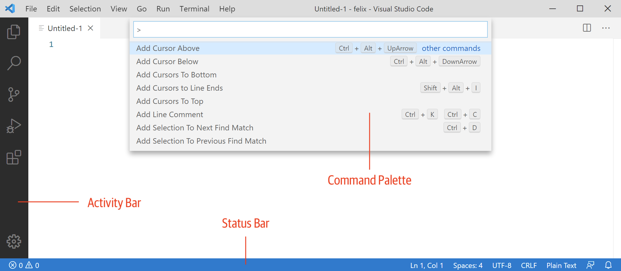
Figure 2-4. VS Code
- Activity Bar
-
On the left-hand side, you see the Activity Bar with the following icons from top to bottom:
-
Explorer
-
Search
-
Source Control
-
Run
-
Extensions
-
- Status Bar
-
At the bottom of the editor, you have the Status Bar. Once you’ll have the configuration completed and edit a Python file, you will see the Python interpreter show up there.
- Command Palette
-
You can show the Command Palette via
F1or with the key combinationCtrl-Shift-P(Windows) orCommand-Shift-P(macOS). If you are unsure about something, your first stop should always be the Command Palette as it gives you easy access to almost everything you can do with VS Code. For example, if you are looking for keyboard shortcuts, simply type inkeyboard shortcuts, select the entryHelp: Keyboard Shortcuts Referenceand hitEnter.
With VS Code installed, let’s configure it to work properly with Python files!
Configuration
By installing VS Code, you have great text editor, but to make it work nicely with Python, there are a few more things to configure: Click on the Extensions icon on the Activity Bar and search for Python. Install the official Python extension that shows Microsoft as the author. It will take a moment to install and in the end, you may need to click the Reload Required button to finish—alternatively, you can also restart VS Code completely. Finalize the configuration according to your platform:
- Windows
-
Open the Command Palette and type:
default shell. HitEnteron the entry that appears:Terminal: Select Default Shell. In the dropdown menu, selectCommand Promptand confirm by hittingEnter. This is required as VS Code otherwise can’t properly activate Conda environments. - macOS
-
Open the Command Palette and type:
shell command. HitEnteron the entry that appears:Shell Command: Install 'code' command in PATH. This is required so that you can run VS Code directly from the command line.
And that’s all that’s required on the configuration side for now. Like before with Jupyter notebooks, the next sections show you how to write and run a first Python script.
A First Script
While you can open VS Code via the Start menu on Windows or Launchpad on macOS, it’s often faster and easier to open VS Code from the command line. It can also prevent permission or environment issues that sometimes happen. Therefore, open a new command line and change into the directory where you want to work, then instruct VS Code to open the current directory (represented by the dot):
$ cd C:Usersusernamepython-for-excelch02
$ code .
With VS Code running, click on the Explorer in the Activity Bar. When you hover over the file list, you will see the New File button appear as shown in Figure 2-5. Click on New File and call your file hello_world.py, then hit Enter. Once it opens in the editor, write the following line of code:
print("hello world!")
Remember that Jupyter notebooks conveniently print the return value of the last line automatically? When you run a traditional Python script, you need to tell Python explicitly what to print, which is why you need to use the print function here. In the Status Bar you should now see your Python version, e.g. Python 3.8.3 64-bit ('base': Anaconda). If you click on it, the Command Palette will open and allow you to select a different Python interpreter if you have more than one (this includes Conda environments). Your setup should now look like in Figure 2-5.

Figure 2-5. VS Code with hello_world.py open
Before moving on to the next section, where you will learn how to run this code, make sure to save the script by hitting Ctrl-S on Windows or Command-S on macOS.
Run the Script
With Jupyter notebooks, we could simply select a cell and hit Shift-Enter to run that cell. With VS Code, you can run your code from either the command line or by clicking the run button. Running Python code from the command line is how you most likely run scripts once they are in production, i.e. scripts that you are not actively editing anymore, so it’s important to know how this works:
- Command Line
-
Open a command line,
cdinto the directory with the script, then run the script like so:$ cd C:Usersusernamepython-for-excelch02 $ python hello_world.py hello world!
The last line is the output that is printed by the script. Note that if you are not in the same directory as your Python file, you need to use the full path to your Python file:
$ python C:Usersusernamepython-for-excelch02hello_world.py
hello world!
Long File Paths on the Command Line
A convenient way to deal with long file paths is to drag and drop the file onto your command line. This will write the full path wherever the cursor is.
- Command Line in VS Code
-
You don’t need to switch away from VS Code to work with the command line: VS Code has an integrated command line that you can show via the keyboard shortcut
Ctrl-`or viaView>Terminal. Since it opens in the project folder, you can run it without changing the directory first:$ python hello_world.py hello world!
- Run Button in VS Code
-
Knowing how to run a Python script from the command line is important and often used but while you are developing in VS code, there is an easier way: if you have a Python file open in VS Code, there is a small green play button at the top right, see Figure 2-5. When you click on it, it will open the Terminal at the bottom automatically and run the code there.
At this point, you know how to create, edit and run Python files in VS Code. Another helpful feature is the ability to step through your code line by line: the next section introduces you to the VS Code debugger.
Debugging
If you ever used the VBA debugger in Excel, I have good news for you: debugging with VS Code is a very similar experience. Let’s make the hello_world.py sample slightly longer by adding a few lines of code:
("hello world!")a=1b=2c=a+b(c)
Click on the left margin next to where it shows line number 5. A red dot will appear: this is your breakpoint where code execution will be paused. Hit F5 to start debugging. The Command Panel will appear with a selection of debug configurations. Choose Python File to debug the currently active file. This will run the code with the debugger and once execution reaches the line with the breakpoint, that line will be highlighted and code execution pauses. Also, the status bar turns orange during debugging as shown in Figure 2-6.

Figure 2-6. VS Code with the debugger stopped at the breakpoint
In the Variables Pane that pops up on the left, you can see the values of the variables. Alternatively, you can also hover over a variable in the source code and get a tooltip with its value. At the top, you will see the Debug Toolbar that gives you access to the following buttons: Continue, Step Over, Step Into, Step Out, Restart, Stop. When you hover over them, you will also see the keyboard shortcuts. Let’s see what each of these buttons does:
- Step Over
-
The debugger will advance one line.
Step Overmeans that the debugger will not step through lines of code that are not part of your current scope. For example, it will not step through the code of a function that you call. - Continue
-
This continues to run the program until it either hits the next breakpoint or the end of the program. If it reaches the end of the program, the debugging process will stop.
- Step Into
-
If you have code that calls e.g. a function,
Step Intowill cause the debugger to step into that function. If the function is in a different file, the debugger will open this file for you. - Step Out
-
If you stepped into e.g. a function with
Step Into, this causes the debugger to return to the next higher scope until eventually, you will be back on the highest level from where you calledStep Intoinitially. - Restart
-
This will stop the current debug process and start a new one from the beginning.
- Stop
-
This will stop the current debug process.
Now that you know what each button does, click on Step Over to advance one line and see how the c variable appears in the Variable Pane, then finish this debugging exercise by clicking on Continue.
Debug configuration
You can also save the debugging configuration so that the Command Panel will not pop up to ask you about the configuration every time you hit F5: click on the Run icon in the Activity Bar, then press the button create a launch.json file. The Command Panel will pop up: choose again Python File. This will create the launch.json file under a directory called .vscode. You can now hit F5 and the debugger will start right away. If you ever need to change the configuration or want to get the Command Panel pop up again, edit or delete the launch.json file in the .vscode directory.
So far, we used VS Code to edit our first Python script hello_world.py. VS Code, however, is also capable of running your Jupyter notebooks! The next section shows you how.
Jupyter Notebooks in VS Code
VS Code allows you to run Jupyter notebooks directly. That is, it’s an alternative to the web browser from the previous section. On top of that, VS Code offers a convenient variable explorer as well as options to transform the notebook into standard Python files without losing the cell functionality. This will make it easier to use some VS Code features like the debugger. Let’s get started and run our previous notebook in VS Code!
Run Jupyter notebooks
Click the Explorer icon on the Activity Bar and open first_notebook.ipynb from before. This will automatically start the Jupyter server in the background. You will see its status on the top right of your notebook. If it is the first time that you launch a notebook in the current VS Code session, it might take a moment until it is running. If you’d rather like to start a new Jupyter notebook, simply create a new file with the .ipynb file extension instead. The layout of the notebook looks a bit different from before to match the rest of VS Code, but otherwise, it works the same including all the keyboard shortcuts. Let’s add a new cell at the end with the following content:
In[9]:a=1b=[[1,2],[3,4]]
The variable b is a nested list, something I will explain in detail in Chapter 3. Run the cell via Shift-Enter, then click on the calculator button in the menu at the top of the notebook: this will open the Variable Explorer where you can see the values of all variables that are currently existing on the notebook kernel, see Figure 2-7. That is, you will only find variables from cells that have been run.
Saving notebooks in VS Code
To save notebooks in VS Code, you need to use the save button at the top of the notebook. Ctrl-S or File > Save won’t work.
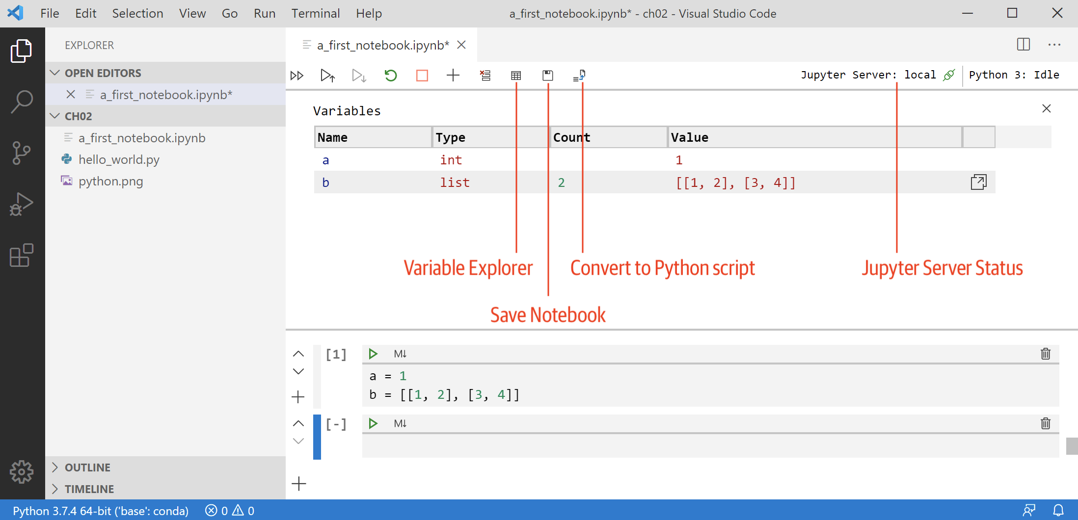
Figure 2-7. Jupyter notebook variable explorer
If you use array data structures like the nested list of variable b, you can double-click the variable: this will open the Data Viewer and give you a familiar spreadsheet-like view. Figure 2-8 shows the Data Viewer after double-clicking variable b.

Figure 2-8. Jupyter notebook data viewer
While VS Code allows you to run Jupyter notebooks as is, it also allows you to transform the notebooks into normal Python files—without losing your cells. I’ll explain next how this works.
Python files with code cells
VS Code allows you to transform Jupyter notebooks into standard Python files that use a special comment to denote cells: # %%. The same syntax is also supported in Spyder and PyCharm (see “Alternative Tools”). Comments in Python start with # as I will introduce properly in Chapter 3. To convert a Jupyter notebook, open it and hit the Convert and save to a Python script button in the menu at the top of the notebook. You can also write your Python files from scratch by using the following syntax for Code and Markdown cells, respectively. Create a new file called cells.py with this content:
# %%3+4# %% [markdown]# # This is Markdown Cell## Some markdown content
Markdown cells need to start with # %% [markdown] and require the whole cell to be marked as comment. If you want to run such a file as notebook, click on the Run Below link that appears when you hover over the first cell. This will open up the Python Interactive Window to the right, see Figure 2-9.
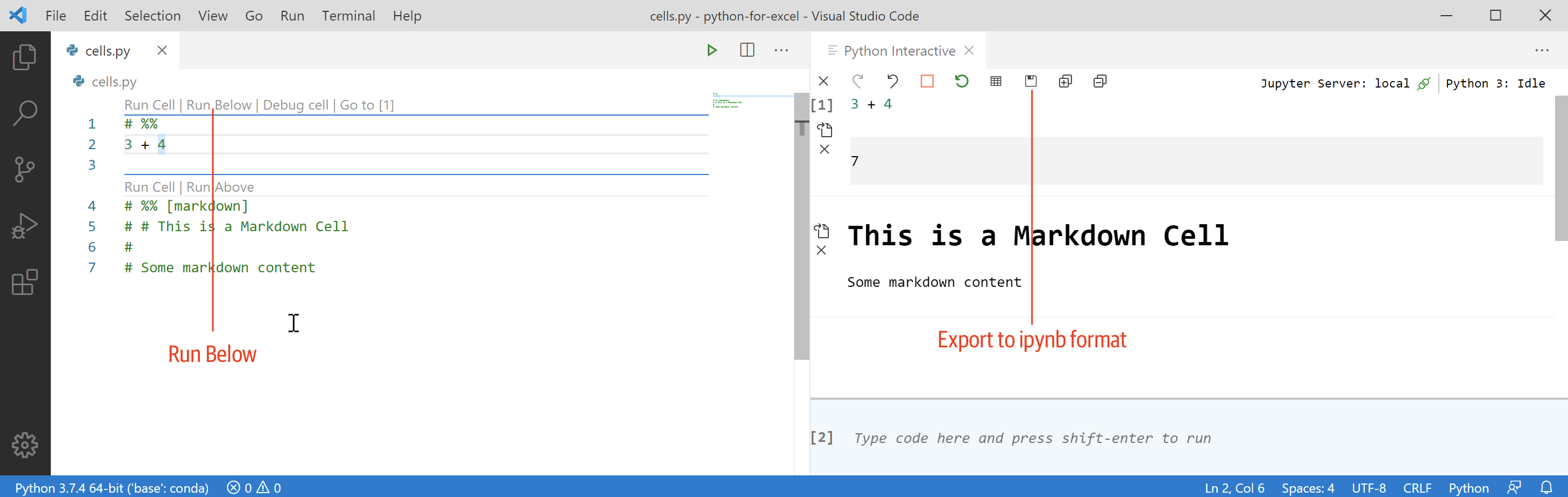
Figure 2-9. Python interactive window
The Python Interactive Window is again shown as notebook. This allows you to click the Save button at the top of the Python Interactive Window to export your file in the ipynb format. The Python Interactive Window also offers you a cell at the bottom from where you can execute code interactively, very much like the REPL from the beginning of this chapter. Depending on your use case, using Python files instead of notebooks can have certain benefits like being able to use the VS Code debugger. Working with standard Python files also makes it way easier to track your files with Git version control as you are sure to only track your input cells to version control, not the output cells that can add a lot of noise between versions.
Conclusion
In this chapter, I showed you how to use the three essential tools that we will work with in this book: the command line, Jupyter notebooks and VS Code. We also installed Python via the Anaconda distribution and started to edit and run small code snippets via Python scripts and Jupyter notebooks.
I recommend you to get comfortable with the command line as it will give you a lot of power once you get used to it. However, the ability to run Jupyter notebooks in the cloud is also very comfortable: it allows you to follow the code samples of this book with the click of a button. This should even work with your corporate computer, where you may not be able to easily install additional software.
With a working development environment, you are now ready to tackle the next chapter: it teaches you enough Python to be able to follow the rest of the book.
1 32-bit systems only exist with Windows and have become rare. An easy way to find out which Windows version you have is by going to the C: drive in the File Explorer. If you can see both the Program Files and Program Files (x86) folders, you are on a 64-bit version of Windows. If you can only see the Program Files folder, you are on a 32-bit system.