
Evolutionary Optimization Through PAC Learning
Forbes J. Burkowski Department of Computer Science, University of Waterloo, Canada
Abstract
Strategies for evolutionary optimization (EO) typically experience a convergence phenomenon that involves a steady increase in the frequency of particular allelic combinations. When some allele is consistent throughout the population we essentially have a reduction in the dimension of the binary string space that is the objective function domain of feasible solutions. In this paper we consider dimension reduction to be the most salient feature of evolutionary optimization and present the theoretical setting for a novel algorithm that manages this reduction in a very controlled albeit stochastic manner. The ”Rising Tide Algorithm” facilitates dimension reductions through the discovery of bit interdependencies that are expressible as ring-sum-expansions (linear combinations in GF2). When suitable constraints are placed on the objective function these interdependencies are generated by algorithms involving approximations to the discrete Fourier transform (or Walsh Transform). Based on analytic techniques that are now used by researchers in PAC learning, the Rising Tide Algorithm attempts to capitalize on the intrinsic binary nature of the fitness function deriving from it a representation that is highly amenable to a theoretical analysis. Our overall objective is to describe certain algorithms for evolutionary optimization as heuristic techniques that work within the analytically rich environment of PAC learning. We also contend that formulation of these algorithms and empirical demonstrations of their success should give EO practitioners new insights into the current traditional strategies.
1 Introduction
The publication of L. Valiant’s ”A Theory of the Learnable” (Valiant, 1984) established a solid foundation for computational learning theory because it provided a rigorous framework within which formal questions could be posed. Subsequently, computational learning has spread to other areas of research, for example, (Baum, 1991), and (Anthony, 1997) discuss the application of Valiant’s PAC (Probably Approximately Correct) model to learnability using neural nets.
The focus of this paper will be to provide an extension of the PAC model that we consider beneficial for the study of Evolutionary Algorithms (EAs). Learning is not new to EAs, see (Belew, 1989) and (Sebag and Schoenauer, 1994). Other research has addressed related issues such as discovery of gene linkage in the representation (Harik, 1997) and adaptation of crossover operators (Smith and Fogarty, 1996) and (Davis, 1989). See (Kargupta and Goldberg, 1997) for another very interesting study. The work of (Ros, 1993) uses genetic algorithms to do PAC learning. In this paper we are essentially going in the opposite direction: using PAC learning to do evolutionary computation.
The benefits of placing evolutionary computation, and particularly genetic algorithms, in a more theoretical framework have been a recurrent research objective for more than a decade. Various researchers have striven to get more theoretical insights into representation of feasible solutions especially with regard to interdependencies among the bits in a feasible solution, hereafter referred to as a genome. While many papers have dealt with these concerns, the following references should give the reader a reasonable perspective on those issues that are relevant to this paper:
(Liepins and Vose, 1990) discusses various representational issues in genetic optimization. The paper elaborates the failure modes of a GA and eventually discusses the existence of an affine transformation that would convert a deceptive objective function to an easily optimizable objective function. Later work (Vose and Liepins, 1991) furthers their examination of schema analysis by examining how the crossover operator interacts with schemata. A notable result here: ”Every function has a representation in which it is essentially the counting 1’s problem”. Explicit derivation of the representation is not discussed.
(Manela and Campbell, 1992) considers schema analysis from the broader viewpoint provided by abstract harmonic analysis. Their approach starts with group theoretic ideas and concepts elaborated by (Lechner, 1971) and ends with a discussion about epistasis and its relation to GA difficulty.
(Radcliffe, 1992) argues that for many problems conventional linear chromosomes and recombination operators are inadequate for effective genetic search. His critique of intrinsic parallelism is especially noteworthy.
(Heckendorn and Whitley, 1999) do extensive analysis of epistasis using the Walsh transform.
Another promising line of research considers optimization heuristics that learn in the sense of estimating probability distributions that guide further exploration of the search space. These EDA’s (Estimation of Distribution Algorithms) have been studied in (Mühlenbein and Mahnig, 1999) and (Pelikan, Goldberg, and Lobo, 1999).
1.1 Overview
The outline of this paper is as follows: Section 2 gives a short motivational ”sermon” on the guiding principles of our research and essentially extends some of the concerns discussed in the papers just cited. The remainder of the paper is best understood if the reader is familiar with certain results in PAC learning and so, trusting the patience of the reader, we quickly present in Section 3 some required PAC definitions and results. Section 4 presents our motivation for using the PAC model and Section 5 introduces the main theme of the paper: the link between PAC and EO. Sections 6 and 7 discuss some novel EO operators that rely on an approximation to the discrete Fourier transform while Section 8 presents some ideas on how these approximations can be calculated. Section 9 presents more EO technique, specifically dimension reduction and Section 10 summarizes the RTA, an evolutionary optimization algorithm that is the focal point of the paper. Some empirical results are reviewed in Section 11 while Section 12 considers some theory that indicates limitations of our algorithm. Some speculative ideas are also presented. Finally, Section 13 presents conclusions.
2 Motivation
As noted by (Vose, 1999), the ”schema theorem” explains virtually nothing about SGA behaviour. With that issue put aside, we can go on to three other issues that may also need some ”mathematical tightening” namely: positional bias and crossover, deception, and notions of locality. In attempting to adopt a more mathematically grounded stance, this paper will adhere to certain views and methodologies specified as follows:
2.2 Opinions and Methods
Positional Bias and Crossover
Evolutionary operators such as one-point crossover are inherently sensitive to bit order. For example, adjacent bits in a parent are very likely to end up as adjacent bits in a child genome. Consequently, navigation of the search space, while stochastic, will nonetheless manifest a predisposition for restricted movement through various hyper-planes of the domain, an unpredictable phenomenon that may provide unexpected advantages but may also hamper the success of an optimization algorithm. These are the effects of positional bias, a term described in (Eshelman, Caruana, and Schaffer, 1989). The usual description of a Genetic Algorithm is somewhat ill posed in the sense that there is no recommendation and no restriction on the bit order of a representation. With this ”anything goes” acceptance in the setup of a problem, we might suspect that choice of bit representation involves more art than science. More significant from an analytic view point is that it is difficult to predict the extent to which the success of the GA is dependent on a given bit representation.
Methodology 1: Symmetry of bit processing The position taken in this paper is that an evolutionary operator should be ”an equal opportunity bit processor”. Although there may be practical advantages to moving adjacent bits from a parent to a child during crossover we do not depend on such adjacency unless it can be explicitly characterized by the definition of the objective function.
With this approach, uniform crossover is considered acceptable while single point crossover is avoided. Later, we introduce other operators that exhibit a lack of positional bias.
The main concern is to establish a ”level playing field” when evaluating the ability of EO algorithms. If bit adjacency helps in a practical application then this is fine. If its effects cannot be adequately characterized in an empirical study that is comparing two competing algorithms, then it is best avoided.
Deception
Considering the many definitions of deception, the notion of deception is somewhat murky but is nonetheless promoted by a certain point of view that seems to accuse the wrong party, as if to say: ”The algorithm is fine, it’s just that the problem is deceptive”. As noted by (Forrest and Mitchell, 1993) there is no generally accepted definition of the term ”deception”. They go on to state that: ”strictly speaking, deception is a property of a particular representation of a problem rather than of the problem itself. In principle, a deceptive representation could be transformed into a non-deceptive one, but in practice it is usually an intractable problem to find the appropriate transformation.”
Methodology 2: Reversible Transformations We adopt the approach that a given bit representation for a problem should be used primarily for evaluation of the objective function. More to the point, it may be best to apply evolutionary operators to various transformations of these bits. While recognizing the intractability of a computation designed to secure a transformation that would eliminate deception, it should also be recognized that many of the problems given to a GA are themselves intractable. Accordingly, one should at least be open to algorithms that may reduce the complexity of a problem if an easy opportunity to do so arises through the application of a reversible transformation.
Notions of Locality
In this paper we try to avoid any explicit use or mention of a landscape structure imposed by evolutionary operators. We regard the {0, 1}n search space as the ultimate in symmetry: all possible binary strings in a finite n-dimensional space. As such, it lacks any intrinsic neighbourhood structure. Furthermore, we contend that it is beneficial to avoid an ad hoc neighbourhood structure unless such a neighbourhood is defined by a metric that is somehow imposed by the objective function itself. To express this more succinctly: Given an arbitrary function F(x) defined on {0, 1}n there is, from the perspective of mathematical analysis, absolutely no justification for a neighbourhood-defining distance measure in the domain of F(x) unless one has extra knowledge about the structure of F(x) leading to a proper definition of such a metric.
This is in contrast to the case when F(x) is a continuous function mapping some subset of the real line to another subset of the real line. This is such a powerful and concise description of the organizational structure of a mapping between two infinite sets that we gladly accept the usual underlying Euclidean metric for the domain of F(x). Now, although this indispensable metric facilitates a concise description of the continuous mapping, it also causes us to see the fluctuations in F(x) as possibly going through various local optima, a characteristic of F that may later plague us during a search activity for a global optimum.
Perhaps due to this on-going familiarity with neighbourhood structures associated with continuous functions, many researchers still strive to describe a mapping from points in a {0, 1}n search space to the real line as somehow holding local and global distinctions. This is typically done by visualizing a ”landscape” over a search domain that is given a neighbourhood structure consistent with the evolutionary operators. For example, neighbourhood distance may be defined using a Hamming metric or by essentially counting the number of applications of an operator in going from point x to point y in the search domain. But the crucial question then arises: Why should we carry over to functions defined on the finite domain {0, 1}n any notion of a metric and its imposed, possibly restrictive, neighborhood structure unless that structure is provably beneficial?
Methodology 3: Recognition of Structure Progress of an iterative search algorithm will require the ability to define subsets in the search space. As described below, we do this by using algorithms that strive to learn certain structural properties of the objective function. Moreover, these algorithms are not influenced by any preordained notion of an intrinsic metric that is independent of the objective function.
An approach that is consistent with Methodology 3 would be to deploy the usual population of bit strings each with a calculated fitness value obtained via the objective function. The population is then sorted and evolutionary operators are invoked to generate new offspring by essentially recognizing patterns in the bit strings that correspond to high fitness individuals, contrasting these with the bit patterns that are associated with low fitness individuals. If this approach is successful then multi-modality essentially disappears but of course one does have to contend with a possibly very difficult pattern recognition problem.
It should be stated that these methodologies are not proposed to boost the speed of computation but rather to provide a kind of ”base line” set of mathematical assumptions that are not dependent on ill-defined but fortuitous advantages of bit adjacency and its relationship to a crossover operator.
3 PAC Learning Preliminaries
Our main objective is to develop algorithms that do evolutionary optimization of an objective function F(x) by learning certain properties of various Boolean functions that are derived from F(x). The formulation of these learning strategies is derived from PAC learning principles. The reader may consult (Kearns and Vazirani, 1994) or (Mitchell, 1997) for excellent introductions to PAC learning theory. Discussing evolutionary optimization in the setting of PAC learning will require a merging of terminology used in two somewhat separate research cultures. Terms and definitions from both research communities have been borrowed and modified to suit the anticipated needs of our research (with apologies to readers from both communities).
Our learning strategy assumes that we are in possession of a learning algorithm that has access to a Boolean function f(x) mapping X = {0, 1}n to {–1, +1}. The algorithm can evaluate f(x) for any value x ∈ X but it has no additional knowledge about the structure of this function. After performing a certain number of function evaluations the algorithm will output an hypothesis function h(x) that acts as an ![]() -approximation of f(x).
-approximation of f(x).
Definition: ![]() -approximation
-approximation
Given a pre-specified accuracy value ![]() in the open interval (0, 1), and a probability distribution D(x) defined over X, we will say that h(x) is an
in the open interval (0, 1), and a probability distribution D(x) defined over X, we will say that h(x) is an ![]() -approximation for f(x) if f(x) and h(x) seldom differ when x is sampled from X using the distribution D. That is:
-approximation for f(x) if f(x) and h(x) seldom differ when x is sampled from X using the distribution D. That is:
Definition: PAC learnable
We say that a class ![]() of representations of functions (for example, the class DNF) is PAC learnable if there is an algorithm
of representations of functions (for example, the class DNF) is PAC learnable if there is an algorithm ![]() such that for any
such that for any ![]() , δ in the interval (0, 1), and any f in
, δ in the interval (0, 1), and any f in ![]() we will be guaranteed that with a probability at least 1 – δ, algorithm
we will be guaranteed that with a probability at least 1 – δ, algorithm ![]() (f,
(f, ![]() , δ) produces an
, δ) produces an ![]() -approximation h(x) for f(x). Furthermore, this computation must produce h(x) in time polynomial in n, 1/
-approximation h(x) for f(x). Furthermore, this computation must produce h(x) in time polynomial in n, 1/![]() , 1/δ, and s the size of f. For a DNF function f, size s would be the number of disjunctive terms in f.
, 1/δ, and s the size of f. For a DNF function f, size s would be the number of disjunctive terms in f.
Theory in PAC learning is very precise about the mechanisms that may be used to obtain information about the function being learned.
Definition: Example Oracle
An example oracle for f with respect to D is a source that on request draws an instance x at random according to the probability distribution D and returns the example < x, f (x)>.
Definition: Membership Oracle
A membership oracle for f is an oracle that simply provides the value f(x) when given the input value x.
The Discrete Fourier Transform
The multidimensional discrete Fourier transform (or Walsh transform) is a very useful tool in learning theory. Given any x ∈ X, with x represented using the column vector: (x1, x2,…, xn), and a function f : X → R, we define the Fourier transform of f as:
where the parity functions tu : X → {–1, +1} are defined for u ∈ X as:
So, tu (x) has value –1 if the number of indices i at which ui = xi = 1 is odd, and 1 otherwise.
The set {tu (x)}x ![]() X is an orthonormal basis for the vector space of real-valued functions on X. We can recover f from its transform by using:
X is an orthonormal basis for the vector space of real-valued functions on X. We can recover f from its transform by using:
This unique expansion of f(x) in terms of the parity basis tu(x) is its Fourier series and the sequence of Fourier coefficients is called the spectrum of f(x).
Definition: Large Fourier Coefficient Property
Consider Z a subset of X. For a given f(x) and θ > 0, we will say that Z has the large Fourier coefficient property (Jackson, 1995, pg. 47) if:
1. For all v such that ![]() we have v ∈ Z and
we have v ∈ Z and
2. for all v ∈ Z, we have ![]()
Now the Fourier transform ![]() is a sum across all x ∈ X. This involves an amount of computation that is exponential in n. To be of practical use we need a lemma from (Jackson, 1995) that is an extension of earlier work done in (Kushilevitz and Mansour, 1993).
is a sum across all x ∈ X. This involves an amount of computation that is exponential in n. To be of practical use we need a lemma from (Jackson, 1995) that is an extension of earlier work done in (Kushilevitz and Mansour, 1993).
Lemma 1
There is an algorithm KM such that, for any function f : X → R, threshold θ > 0, and confidence δ with 0 < δ < 1, KM returns, with probability at least 1 – δ, a set with the large Fourier coefficient property. KM uses membership queries and runs in time polynomial in n, 1/θ, log(1/δ) and maxx![]() X |f(x)|.
X |f(x)|.
The large Fourier coefficient property provides a vital step in the practical use of the discrete Fourier transform. We can take a given function f and approximate it with a function fz(x) defined as:
with a set size |Z| that is not exponential in size.
Using the results of Lemma 1 Jackson proved that there is an algorithm that finds an ![]() –approximation to a DNF function with
–approximation to a DNF function with  Since
Since ![]() is close to 1/2 instead of close to 1, it is necessary to employ a boosting algorithm (Freund, 1990) so as to increase the accuracy of the
is close to 1/2 instead of close to 1, it is necessary to employ a boosting algorithm (Freund, 1990) so as to increase the accuracy of the ![]() -approximator.
-approximator.
Jackson’s algorithm, called the Harmonic Sieve, expresses the ![]() –approximation h(x) as a threshold of parity (TOP) function. In general, a TOP representation of a multidimensional Boolean function f is a majority vote over a collection of (possibly negated) parity functions, where each parity function is a ring-sum-expansion (RSE) over some subset of f’s input bits. We will assume RSE’s reflect operations in GF2 and are Boolean functions over the base {Λ, ⊕, 1} restricted to monomials (for example, x1 ⊕ x5 ⊕ x 31) (Fischer and Simon, 1992). The main idea behind Jackson’s Harmonic Sieve is that the RSE’s required by the h(x) TOP function are derived by calculating locations of the large Fourier coefficients. The algorithm ensures that the accurate determination of these locations has a probability of success that is above a prespecified threshold of 1 – δ. The algorithm uses a recursive strategy that determines a sequence of successive partitions of the domain space of the Fourier coefficients. When a partition is defined, the algorithm applies Parseval’s Theorem in conjunction with Hoeffding’s inequality to determine whether or not it is highly likely that a subpartition contains a large Fourier coefficient. If so, the algorithm will recursively continue the partitioning of this subpartition. The important result in Jackson’s thesis is that finding these large coefficients can be done in polynomial time with a sample size (for our purposes, population size) that is also polynomial in n, s, and 1/
–approximation h(x) as a threshold of parity (TOP) function. In general, a TOP representation of a multidimensional Boolean function f is a majority vote over a collection of (possibly negated) parity functions, where each parity function is a ring-sum-expansion (RSE) over some subset of f’s input bits. We will assume RSE’s reflect operations in GF2 and are Boolean functions over the base {Λ, ⊕, 1} restricted to monomials (for example, x1 ⊕ x5 ⊕ x 31) (Fischer and Simon, 1992). The main idea behind Jackson’s Harmonic Sieve is that the RSE’s required by the h(x) TOP function are derived by calculating locations of the large Fourier coefficients. The algorithm ensures that the accurate determination of these locations has a probability of success that is above a prespecified threshold of 1 – δ. The algorithm uses a recursive strategy that determines a sequence of successive partitions of the domain space of the Fourier coefficients. When a partition is defined, the algorithm applies Parseval’s Theorem in conjunction with Hoeffding’s inequality to determine whether or not it is highly likely that a subpartition contains a large Fourier coefficient. If so, the algorithm will recursively continue the partitioning of this subpartition. The important result in Jackson’s thesis is that finding these large coefficients can be done in polynomial time with a sample size (for our purposes, population size) that is also polynomial in n, s, and 1/![]() . Unfortunately, the degrees of the polynomials are rather high for practical purposes. However, recent work by (Bshouty, Jackson, and Tamon, 1999) gives a more efficient algorithm, thus showing that Jackson’s Harmonic Sieve can find the large Fourier coefficients in time Ο(ns4/
. Unfortunately, the degrees of the polynomials are rather high for practical purposes. However, recent work by (Bshouty, Jackson, and Tamon, 1999) gives a more efficient algorithm, thus showing that Jackson’s Harmonic Sieve can find the large Fourier coefficients in time Ο(ns4/![]() 4) working with a sample size of Ο(ns2/
4) working with a sample size of Ο(ns2/![]() 4).
4).
Before going any further, we introduce some additional terminology. Each u ∈ X is a bit sequence that we will refer to as a parity string. Corresponding to each parity string we have a parity function tu (x). Note that for Boolean f we have ![]() where E denotes the expectation operator and so the expression represents the correlation of f and tu with respect to the uniform distribution. We will then regard
where E denotes the expectation operator and so the expression represents the correlation of f and tu with respect to the uniform distribution. We will then regard ![]() as representing the correlation of the parity string u.
as representing the correlation of the parity string u.
4 Why We Should Work in a PAC Setting
Our motivation for adopting a PAC learning paradigm as a setting for evolutionary optimization involves the following perceived benefits:
1. A Necessary Compromise
A PAC setting deliberately weakens the objectives of a learning activity:
i) In a certain sense the final answer may be approximate, and
ii) the algorithm itself has only a certain (hopefully high) probability of finding this answer.
Although life in a PAC setting seems to be very uncertain, there is an advantage to be obtained by this compromise. We benefit through the opportunity to derive an analysis that specifies, in probabilistic terms, algorithmic results that can be achieved in polynomial time using a population size that also has polynomial bounds.
2. Learning the Structure of the Objective Function
Most evolutionary algorithms simply evaluate the objective function F(x) at various points in the search space and then subject these values to further operations that serve to distinguish high fitness genomes from low fitness genomes, for example, by building a roulette wheel for parent selection. The central idea of our research is that by applying a learning algorithm to the binary function f(x) = sgn(F(x)) we will derive certain information that is useful in an evolutionary optimization of F(x). In particular, the derivation of a RSE can point the way to transformations of the domain space that hopefully allow dimension reduction with little or no loss of genomes having high fitness.
3. In Praise of Symmetry
The tools now present in the PAC learning community hold the promise of defining evolutionary operators that are free of bit position bias since learning algorithms typically work with values of Boolean variables and there is no reliance on bit string formats.
4. Algorithmic Analysis Related to Complexity
Learning theory has an excellent mathematical foundation that is strongly related to computational complexity. Many of the theorems work within some hypothetical setting that is characterized by making assumptions about the complexity of a function class, for example, the maximum depth and width of a circuit that would implement a function in the class under discussion.
5 PAC Learning Applied to Evolutionary Optimization
The main goal of this paper is to demonstrate that there is a beneficial interplay between Evolutionary Optimization and PAC learning. We hope to use PAC learning as a basis for analytical studies and also as a toolkit that would supply practical techniques for the design of algorithms. The key idea is that a learning exercise applied to the objective function provides an EO algorithm with valuable information that can be used in the search for a global optimum.
There is an obvious connection between an example oracle used in PAC learning and the population of genomes used in genetic algorithms. However, in using PAC learning, it may be necessary to maintain a population in ways that are different from the techniques used in ” traditional” EO. In our approach to optimization we will need values of the objective function that provide examples of both high fitness and low fitness, or expressed in terms of an adjusted, objective function, we will need to maintain two subpopulations, one for positive fitness genomes and another for negative fitness genomes. Learning techniques would then aid an optimization algorithm that attempts to generate ever-higher fitness values while avoiding low (negative) fitness.
The adjustment of the fitness function F(x), shifted so that ![]() is done to provide a sign function f(x) that is reasonably balanced in its distribution of positive and negative values. This does not change the location of the global optimum and it increases the correlation between the signum function f(x) and the parity functions tu(x) which are also balanced in this way. The deliberate strategy to provide both positive and negative examples of the objective function is motivated by the idea that these examples are needed since dimension reduction should attempt to isolate high fitness and at the same time avoid low (i.e. negative) fitness. This approach is also consistent with (Fischer and Simon, 1992) which reports that learning RSE’s can be done, with reasonable restrictions on f(x), but one must use both positive and negative examples to guide the learning process.
is done to provide a sign function f(x) that is reasonably balanced in its distribution of positive and negative values. This does not change the location of the global optimum and it increases the correlation between the signum function f(x) and the parity functions tu(x) which are also balanced in this way. The deliberate strategy to provide both positive and negative examples of the objective function is motivated by the idea that these examples are needed since dimension reduction should attempt to isolate high fitness and at the same time avoid low (i.e. negative) fitness. This approach is also consistent with (Fischer and Simon, 1992) which reports that learning RSE’s can be done, with reasonable restrictions on f(x), but one must use both positive and negative examples to guide the learning process.
We next present an informal description of such an optimization algorithm.
5.1 The Rising Tide Algorithm
To appreciate the main strategy of our algorithm in action the reader may visualize the following scenario: In place of hill-climbing imagery, with its explicit or implicit notions of locality, we adopt the mindset of using an algorithm that is analogous to a rising tide. The reader may imagine a flood plane with various rocky outcroppings. As the tide water floods in, the various outcroppings, each in turn, become submerged and, most important for our discussion, the last one to disappear is the highest outcropping.
Before continuing, it is important not to be led astray by the pleasant continuity of this simple scene, which is only used to provide an initial visual aid. In particular it is to be stressed that the justification of the algorithm involves no a priori notion of locality in the search space. In fact, any specification of selected points in the domain {0,1}n is done using a set theoretic approach that will define a sub-domain through the use of constraints that are expressed in terms of ring-sum-expansions, these in turn being derived from computations done on F(x).
From an algorithmic perspective, our task is to provide some type of computational test that will serve to separate the sub-domain that supports positive fitness values from the sub-domain that support negative fitness values. In a dimension reduction step, we then alter the objective function by restricting it to the sub-domain with higher fitness values. An obvious strategy is to then repeat the process to find a sequence of nested sub-domains each supporting progressively higher fitness genomes while avoiding an increasing number of lower fitness genomes.
In summary, the intention of the Rising Tide Algorithm (RTA) is to isolate successive subsets of the search space that are most likely to contain the global maximum by essentially recognizing patterns in the domain made evident through a judicious use of an approximation to the discrete Fourier transform. Of particular note: If a sub-domain that supports positive values can be approximately specified by using a TOP function, then the RSE’s of that function can be used to apply a linear transform to the input variables of F(x). The goal of the transformation would be to give a dimension reduction that is designed to close off the portion of the space that, with high probability, supports negative values of the fitness function. With this dimension reduction we have essentially ”raised the tide”. We have derived a new fitness function with a domain that represents a ”hyperslice” through the domain of the previous objective function. The new fitness function is related to the given objective function in that both have the same global optimum unless, with hopefully very low probability, we have been unfortunate enough to close off a subset of the domain that actually contains the global maximum. If the function is not unduly complex, repeated application of the technique would lead to a sub-domain that is small enough for an exhaustive search.
5.2 The RTA in a PAC Setting
In what follows we will consider the objective function F(x) to be a product of its signum function f(x) and its absolute value:
This is done to underscore two important connections with learning theory. The signum function f(x) is a binary function that will be subjected to our learning algorithm and when properly normalized, the function |F(x)| essentially provides the probability distribution D(x) defined in section 3. More precisely:
Apart from the obvious connection with the familiar roulette wheel construction used in genetic algorithms we see the employment of D(x) as a natural mechanism for an algorithm that seeks to characterize f (x) with the goal of aiding an optimization activity.
It is reasonable to assume that we would want the learning of f (x) to be most accurately achieved for genomes x having extreme fitness values. This directly corresponds to the larger values of the distribution D(x). So, when learning f(x) via an approximation to the discrete Fourier transform of F(x), it will be as if the population has high replication for the genomes with extreme values of fitness.
More to the point, the definition of ![]() –approximation (1) works with f (x) in a way that is consistent with our goals. The heuristic strategy here is that we do not want an
–approximation (1) works with f (x) in a way that is consistent with our goals. The heuristic strategy here is that we do not want an ![]() –approximation of f(x) that is uniform across all x in the search space. The intermediate ”close to zero” values of F(x) should be essentially neglected in that they contribute little to the stated containment-avoidance objectives of the algorithm and only add to the perceived complexity of the function f(x).
–approximation of f(x) that is uniform across all x in the search space. The intermediate ”close to zero” values of F(x) should be essentially neglected in that they contribute little to the stated containment-avoidance objectives of the algorithm and only add to the perceived complexity of the function f(x).
5.3 Leamability Issues
We start with the reaffirmation that the learning of f(x) is important because f(x) is a two valued function that partitions the X domain into two subspaces corresponding to positive and negative values of F(x). The heuristic behind RTA is to attempt a characterization of both of these subspaces so that we can try to contain the extreme positive F(x) values while avoiding the extreme negative F(x) values. Of even more importance is the attempt to characterize F(x) through the succession of different f (x) functions that appear as the algorithm progresses, (more picturesquely: as the tide rises).
The re-mapping of f values from the set {−1, +1} to {1, 0}, done by replacing f with ![]() allows us to see the sign function as a regular binary function. In some cases the leamability of /(x), at least in a theoretical sense, can be guaranteed if f(x) belongs to a class that is known to be learnable. Research in learning theory gives several descriptions of such classes. Three examples may be cited:
allows us to see the sign function as a regular binary function. In some cases the leamability of /(x), at least in a theoretical sense, can be guaranteed if f(x) belongs to a class that is known to be learnable. Research in learning theory gives several descriptions of such classes. Three examples may be cited:
1-RSE*
If f(x) is equivalent to a ring-sum-expansion such that each monomial contains at most one variable but does not contain the monomial 1, then f (x) is learnable (Fischer and Simon, 1992).
DNF
If f(x) is equivalent to a disjunctive normal form then f(x) is PAC learnable assuming the distribution D(x) is uniform (Jackson, 1995) and (Bshouty, Jackson, and Tamon, 1999).
AC0 Circuits
An AC0 circuit consists of AND and OR gates, with inputs x1, x2, …, xn and ![]() Fanin to the gates is unbounded and the number of gates is bounded by a polynomial in n. Depth is bounded by a constant. Leamability of AC0 circuits is discussed in (Linial, Mansour, and Nisan, 1993).
Fanin to the gates is unbounded and the number of gates is bounded by a polynomial in n. Depth is bounded by a constant. Leamability of AC0 circuits is discussed in (Linial, Mansour, and Nisan, 1993).
As noted in (Jackson, 1995), the leamability of DNF is not guaranteed by currently known theory if D(x) is arbitrary. Jackson’s thesis does investigate leamability, getting positive results, when D(x) is a product distribution. For our purposes, we adopt the positive attitude that when there is no clear guarantee of learnability, we at least have some notion about the characterization of an objective function that may cause trouble for our optimization algorithm.
6 Transformation of a Representation
Before presenting the main features of our algorithm we discuss a strategy that allows us to change the representation of a genome by essentially performing an n-dimensional rotation of its representation. The main idea here is that a suitable rotation may allow us to ”dump” the low fitness genomes into a hyper-plane that is subsequently sealed off from further investigation. A compelling visualization of this strategy would be to think of the puzzle known as Rubik’s cube1. By using various rotation operations we can separate or combine corners of the cube in myriad ways placing any four of them in either the same face or in different faces of the cube. Considering the possibilities in 3-space, the transformations in n-space tend to boggle the mind but we need this operational complexity if a rotation is to accomplish the genome separation described earlier.
Transformation of a representation is initiated by collecting a set Z of the parity strings corresponding to the large Fourier coefficients. We then extract from Z a set W of linearly independent w that are at most n in number. These will be used as the rows of a rotation matrix A. If the number of these w is less than n, then we can fill out remaining rows by setting aii = 1 and aij = 0 for off-diagonal elements. The motivation for generating A in this way rests on the following simple observation:
Starting with ![]() we replace x with A−1y to get:
we replace x with A−1y to get:
Now, since AT is nonsingular it possesses a nonsingular inverse, or more noteworthy, it provides a bijective mapping of X onto X. Since u in the last summation will go through all possible n bit strings in X we can replace u with ATu and the equation is still valid. Consequently:
where E is the collection of all n bit strings that have all entries 0 with a single 1 bit. Note that when a particular e vector is multiplied by AT we simply get one of the w in the set W and so ![]() is a large Fourier coefficient. Consequently, if there are only a few large Fourier coefficients2, we might expect the first sum in the last equation to have a significant influence on the value of the objective function. When this is the case, a y value producing a highly fit value for g(y) might be easily determined. In fact, the signs of the large Fourier coefficients essentially spell out the y bit string that will maximize the first sum. We will refer to this particular bit string as the signature of A. For example, if all the large Fourier coefficients in this sum are negative then the value of y will be all l’s and we have the ”ones counting” situation similar to that described in (Vose and Liepins, 1991). So, our main strategy is to generate a non-singular matrix A that will map the typical genome x to a different representation y = Ax. The objective function F(x) then becomes F(A−ly) = g(y) and we hope to isolate the positive values of g(y) by a judicious setting of bits in the y string.
is a large Fourier coefficient. Consequently, if there are only a few large Fourier coefficients2, we might expect the first sum in the last equation to have a significant influence on the value of the objective function. When this is the case, a y value producing a highly fit value for g(y) might be easily determined. In fact, the signs of the large Fourier coefficients essentially spell out the y bit string that will maximize the first sum. We will refer to this particular bit string as the signature of A. For example, if all the large Fourier coefficients in this sum are negative then the value of y will be all l’s and we have the ”ones counting” situation similar to that described in (Vose and Liepins, 1991). So, our main strategy is to generate a non-singular matrix A that will map the typical genome x to a different representation y = Ax. The objective function F(x) then becomes F(A−ly) = g(y) and we hope to isolate the positive values of g(y) by a judicious setting of bits in the y string.
Note that matrix transforms have been discussed earlier by (Battle and Vose, 1991) who consider the notion of an invertible matrix to transform a genome x into a genome y that resides in a population considered to be isomorphic to the population holding genome x. They also note that converting a standard binary encoding of a genome to a Gray encoding is a special case of such a transformation.
Our techniques may be seen as attempts to derive an explicit form for a matrix transformation that is used with the goal of reducing simple epistasis describable as a ring-sum dependency among the bits of a genome. To nullify any a priori advantage or disadvantage that may be present due to the format of the initial representation, knowledge used to construct matrix A is derived only through evaluations of the fitness function F(x). By using F(x) as a ”black box” we are not allowed to prescribe a Gray encoding, for example, on the hunch that it will aid our optimization activity. Instead, we let the algorithm derive the new encoding which, of course, may or may not be a Gray encoding. With these ”rules of engagement” we forego any attempt to characterize those fitness functions that would benefit from the use of a Gray encoding. Instead, we seek to develop algorithms that lead to a theoretical analysis of the more general transformation, for example, the characterization of a fitness function that would provide the derivation of a matrix A that serves to reduce epistasis.
Recalling ”Methodology 2” in Section 2.1, we emphasize some important aspects of our approach: The given genome representation is considered to be only useful for fitness evaluation. Evolutionary operators leading to dimension reduction are usually applied to a transformation of the genome not the genome itself. Although we start with a genome that is the given linear bit string, our initial operations on that string will be symmetric with respect to all bits. Any future asymmetry in bit processing will arise in due course as a natural consequence of the algorithm interacting with F(x). To enforce this approach, operators with positional-bias, such as single point crossover, will be avoided. For similar reasons, we avoid any analysis that deals with bit-order related concepts such as ”length of schemata”.
7 Evolutionary Operators
Equation (9) becomes the starting point for many heuristics dealing with the construction of an evolutionary operator. First some observations and terminology are needed. We will say that a parity string with a large Fourier coefficient (large in absolute value) has a high correlation. This correlation may be very positive or very negative, but in either case, it helps us characterize f(x). Considering equation (9), we will refer to the sum ![]() as the unit vector sum and the last sum
as the unit vector sum and the last sum ![]() will be the high order sum. As noted in the previous section, for a given non-singular matrix A there is an easily derived particular binary vector y, called the signature of A, that will maximize the unit vector sum.
will be the high order sum. As noted in the previous section, for a given non-singular matrix A there is an easily derived particular binary vector y, called the signature of A, that will maximize the unit vector sum.
Before going further, we should note that if A is the identity matrix, then x is not rotated (i.e. y = x), and more importantly, we then see the first sum in equation (9) as holding Fourier coefficients corresponding to simple unit vectors in the given non-rotated space. So, if we retain the original given representation, mutational changes made to a genome by any genetic algorithm essentially involves working with first sum terms that do not necessarily correspond to the large Fourier coefficients. In this light, we see a properly constructed rotational transformation as hopefully providing an edge, namely the ability to directly manipulate terms that are more influential in the first sum of equation (9). Of course, we should note that this heuristic may be overly optimistic in that maximization of the first sum will have ”down-stream” effects on the second sum of equation (9). For example, it is easy to imagine that the signature vector, while maximizing the unit vector sum may cause the high order sum to overwhelm this gain with a large negative value. This is especially likely when the power spectrum corresponding to the Fourier transform is more uniform and not concentrated on a small number of large Fourier coefficients. Our approach is to accept this possible limitation and proceed with the heuristic motivation that the first sum is easily maximized and so represents a good starting point for further exploration of the search space, an exploration that may involve further rotations as deemed necessary as the population evolves.
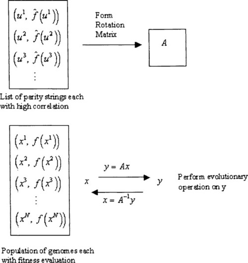
Keeping these motivational ideas in mind, we seek to design an effective evolutionary operator that depends on the use of a rotation matrix A. We have experimented with several heuristics but will discuss only two of them:
Genome creation from a signature
For this heuristic, we generate A by selecting high correlation parity strings using a roulette strategy. We then form the signature y and compute a new positive fitness genome as A−1y. In a similar fashion, the complement of y can be used to generate a new negative fitness genome as A−1y.
Uniform crossover in the rotated space
We start with a matrix A that is created using a greedy approach, selecting the first n high correlation parity strings that will form a singular matrix. We use roulette to select a high fitness parent genome and rotate it so that we calculate its corresponding representation as a y vector. We are essentially investigating how this high fitness genome has tackled the problem of attempting to maximize the unit vector sum while tolerating the downstream effects of the high order sum. The same rotation is performed on another parent and a child is generated using uniform crossover. Naturally, the child is brought back into the original space using the inverse rotation supplied by A−1. Once this is done, we evaluate fitness and do the subtraction to get its adjusted fitness. A similar procedure involving negative fitness parents is done to get negative children.
Figure 1 presents these strategies in diagram form. Note that genome creation from a signature does not use the matrix A directly, but rather its inverse.
8 Finding High Correlation Parity Strings
An implementation that derives the large Fourier coefficients using Jackson’s algorithm involves very extensive calculations and so we have adopted other strategies that attempt to find high correlation parity strings. The main idea here is that the beautiful symmetry of the equations defining the transform and its inverse, leads to the compelling notion that if we can evolve genomes using a parity string population then the same evolutionary operators should allow us to generate parity strings using a genome population.
In going along with this strategy, we have done various experiments that work with two coevolving populations, one for the genomes, and another for the parity strings. The key observation is that the parity strings also have a type of ”fitness” namely the estimation of the correlation value, or Fourier coefficient, associated with the string.
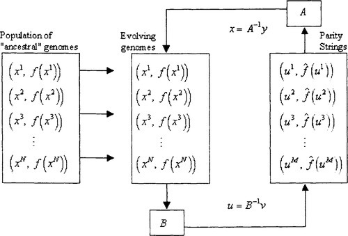
Our initial experiments attempted to implement this in a straightforward manner: the parity string population provided a rotation matrix A used to evolve members of the genome population while the genome population provided a rotation matrix B used to evolve members of the parity string population. Results were disappointing because there is a trap involved in this line of thinking. The estimation of a correlation value is based on a uniform distribution of strings in the genome population. If the two populations are allowed to undergo a concurrent evolution then the genome population becomes skewed with genomes of extreme fitness and eventually the estimation of correlation becomes more and more in error. To remedy this situation we use instead a strategy described by Figure 2. We start with a randomly initialized genome population referred to as the ”ancestral” population. It is used for calculations of correlation estimation and will remain fixed until there is a dimension reduction. The population of evolving genomes is randomly initialized and concurrent evolution proceeds just as described except that all correlation calculations work with the ancestral population. Going back to our definitions in the PAC introduction, the ancestral population essentially makes use of an example oracle while the evolving population continually makes use of a membership oracle. This is illustrated in Figure 2.
A reasonable question is whether we can evaluate the correlation of a parity string using a genome population of reasonable size or will we definitely require an exponential number of genomes to do this properly? To answer this we appeal to a lemma by (Hoeffding, 1963):
Lemma 2
Let X1, X2,…, Xm be independent random variables all with mean μ such that for all i, a ≤ Xi ≤ b. Then for any λ > 0,
To apply this we reason as follows: Suppose we have guessed that v is a high correlation parity string with correlation ![]() and we wish to verify this guess. We would draw a sample X, in our case a population X of x ∈ {0, l}n uniformly at random and compute
and we wish to verify this guess. We would draw a sample X, in our case a population X of x ∈ {0, l}n uniformly at random and compute ![]() where |X| represents the size of the genome population. For this discussion the values of a and b delimit the interval containing the range of values for the function F(x). In Hoeffding’s inequality μ represents the true value of the correlation and the sum is our estimate. Following (Jackson, 1995) we can make this probability arbitrarily small, say less than 6 by ensuring that m is large enough. It is easily demonstrated that the absolute value of the difference will only exceed the tolerance value A with some low probability 6 if we insist that:
where |X| represents the size of the genome population. For this discussion the values of a and b delimit the interval containing the range of values for the function F(x). In Hoeffding’s inequality μ represents the true value of the correlation and the sum is our estimate. Following (Jackson, 1995) we can make this probability arbitrarily small, say less than 6 by ensuring that m is large enough. It is easily demonstrated that the absolute value of the difference will only exceed the tolerance value A with some low probability 6 if we insist that:
This gives us a theoretical guarantee that the population has a size that is at most quadratic in the given parameter values.
9 Dimension Reduction
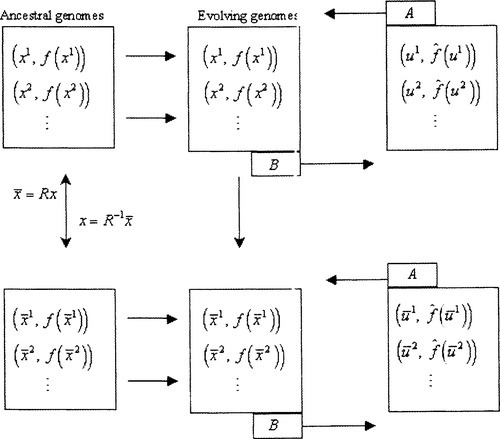
As described in Section 7, application of the evolutionary operators is done with the hope that the evolving populations will produce ever more extreme values. The populations evolve and eventually we obtain the high fitness genomes that we desire. An additional strategy is to recognize exceptionally high correlation parity strings and use them to provide a rotation of the space followed by a ”freezing” of a particular bit in the y representation that essentially closes off half of the search space. This will essentially reduce the complexity of the problem and will present us with a new fitness function working on n – 1 bits instead of n bits. Within this new space we carry on as we did prior to the reduction, doing rotations, fostering mutual evolution, and waiting for the opportunity to do the next dimension reduction. In our implementation of this scheme, the rotation transformation is followed by a permutation transformation that puts the frozen bit into the last bit position of the new representation. While this amounts to some extra computation it certainly makes it easier to follow the progress of the algorithm.
Whenever a rotation and permutation are done we also compute the inverse of this matrix product R to maintain a recovery matrix R−1 that can bring us back to the original representation so that the fitness of the genome can be evaluated. Figure 3 illustrates the data flow involved.
10 The Rising Tide Algorithm
We now summarize the content of the previous sections by describing the sequence of steps in a generic description of the Rising Tide Algorithm.
The Rising Tide Algorithm:
1. Randomly generate two populations of binary strings each a member of {0, 1}n.
2. Use the objective function to evaluate the fitness of each string in the genome population.
3. Adjust each fitness value by subtracting from it the average fitness of all members in the population. These adjusted values define the fitness function F(x) and we further assume that f(x) = sgn(F(x)).
4. Using the genome population as a sample space, calculate an approximation to the correlation value for each parity string in the parity population.
5. Designate the genome population as the ancestral population and duplicate it to form the evolving genome population.
6. Perform evolutionary computations on the parity population. These are facilitated through the construction of a matrix B that is built from a linearly independent set of extreme fitness genome extracted from the evolving genome population. Computation of correlation for a new child parity string is done by working with the ancestral population.
7. Perform evolutionary computations on the genome population. These are facilitated through the construction of a matrix A that is built from a linearly independent set of extreme correlation parity strings extracted from the evolving parity string population.
8. Repeat steps 6 and 7 until a parity string has a correlation that exceeds some prespecified threshold value.
9. Use the high correlation parity string to perform a rotation of the ancestral genome population followed by a bit freeze that will constrain the population to that half of the search space containing the highest fitness genomes. We then generate new genomes to replace those that do not meet the constraints specified by the frozen bits.
10. Repetition of steps 6, 7, 8, and 9 is done until either the evolving genome population converges with no further dimension reduction, or the dimension reduction is carried on to the extent that most of the bits freeze to particular values leaving a few unfrozen bits that may be processed using a straightforward exhaustive search.
11 Empirical Results
Experimental results are still being collected for a variety of problems. At the present time, results are mixed and, it would seem, heavily dependent on the ability of the RTA to generate parity strings with a high level of consistency. Here we consider consistency as the ability to meet the requirements of step (9): providing a separating plane that distinguishes as much as possible, the two subpopulations of high and low fitness. In simple cases such as the DeJong Test Function #1, optimizing F(x,y,z) = x2 + y2+ z2 over the domain –5.12 < x, y, z < 5.12 with x, y, and z represented by 10 bit values, we get very compelling results. Of particular note is the manner in which the global optimum is attained. In Table 1 we present a snapshot of the top ranking genomes at the end of the program’s execution. The first column shows the bit patterns of the genomes that were produced by the final evolving population while the second column shows the same genomes with the recovery transformation applied to produce the original bit representation used for the fitness evaluation which is presented in column 3.
Table 1
Highest Ranking genomes for the 1st DeJong Test Function (Both populations have size 300)
| Genome in: Rotated Form | Original Representation | Fitness |
| 0000000000 0000000000 0000010011 | 1000000000 1000000000 1000000000 | 78.6432 |
| 1010010000 00000000000000010011 | 0111111111 1000000000 1000000000 | 78.5409 |
| 0001101000 0000000000 0000010011 | 1000000000 1000000000 0111111111 | 78.5409 |
| 0000100000 00000000000000010011 | 1000000000 1000000000 1000000001 | 78.5409 |
| 1011111000 0000000000 0000010011 | 0111111111 1000000000 0111111111 | 78.4386 |
| 0100100000 0000000000 0000010011 | 1000000000 1000000001 1000000001 | 78.4386 |
Column 1 tells us that their rotated representations are very similar, having identical bit patterns in the frozen subsequence at the end of each string. More significantly, an inspection of the results reveals that even though a type of convergence has taken place for the rotated genomes, the algorithm has actually maintained several high fitness genomes that, when viewed in the original bit representation, are very different if we choose to compare them using a Hamming metric.
The ability of the population to successfully carry many of the high-fitness genomes to the very end of the run, despite their very different bit patterns, is exactly the type of behaviour that we want. It shows us the Rising Tide Algorithm working as described in section 5.1. However, our current experience with more complex functions demonstrates that isolation of high fitness genomes can be quite difficult but it is not clear whether this is due to an inadequate population size or some inherent inability of the algorithm in evolving high correlation parity strings. Further experiments are being conducted.
12 Discussion and Speculation
Working in GF2 is very convenient. We have the luxury of doing arithmetic operations in a field that provides very useful tools, for example: a linear algebra complete with invertible matrices and Fourier transforms. Nonetheless, the Rising Tide Algorithm is certainly no panacea. Discovery of an optimal rotation matrix is beset with certain difficulties that are related to the mechanisms at work in the learning strategy itself. A key issue underlying the processing of the RTA depends on the fact that the learning algorithm applied to the signum function f(x) will determine a set of parity functions that form a threshold of parity or TOP function. The Boolean output of a TOP is determined by a winning vote of its constituent parity strings. Unfortunately, the subset of the parity strings that win the vote can change from one point to any other in the search space. This reflects the nonlinear behaviour of an objective function. Consequently the derivation of a rotation matrix can be quite demanding. Such a difficulty does not necessarily mean that the strategy is without merit. In fact, the ability to anticipate the “show stopper” carries an advantage not provided by the simple genetic algorithm, which will grind away on any population without any notion of failure. So, a more salutary view would recognize that we should, in fact, expect to meet difficulties and the more clear they are, then the more opportunity we have for meeting the challenge they impose.
A possible approach to handle this problem would be the creation of a tree structure with branching used to designate portions of the search space holding genomes that meet the constraints consistent with particular sets of parity strings (a novel interpretation for speciation studies). A strategy very similar to this has been employed by (Hooker, 1998) in the investigation of constraint satisfaction methods. In this paper, the setting is discrete variable logic instead of parity strings being manipulated in GF2. However, the problems encountered when trying to meet consistency requirements for constraint satisfaction are quite similar to the TOP dilemma. To handle the situation, Hooker describes algorithms that utilize backtracking strategies in so-called k-trees. We intend to carry out further studies to make clearer the interplay between these two problem areas.
As a final speculation, we note that it may be reasonable to see ”locality” defined by such a branching process. It meets our demand that the neighbourhood structure be created by the objective function itself and it also carries a similar notion of being trapped within an area that may lead to sub-optimal solutions.
13 Conclusion
We contend that harmonic analysis and especially PAC learning should have significant theoretical and practical benefits for the design of new evolutionary optimization algorithms. The Fourier spectrum of f(x), its distribution of large coefficients and how this relates to the complexity of optimization, should serve to quantitatively characterize functions that are compatible with these algorithms. Although computationally expensive, the DFT does provide a formal strategy to deal with notions such as epistasis and simple (linear) gene linkage expressible as a ring-sum formula. The future value of such a theoretical study would be to see the structure of the search space expressed in terms of the spectral properties of the fitness function. Our view is that this is, in some sense, a more ”natural” expression of the intrinsic structure of the search space since it does not rely on a neighborhood structure defined by the search operator chosen by the application programmer.
This paper has presented several novel ideas in a preliminary report on an evolutionary algorithm that involves an explicit use of the DFT. A possible optimization algorithm was described with attention drawn to some of the more theoretical issues that provide a bridge between PAC learning and evolutionary optimization. More extensive empirical results will be the subject of a future report.
We contend that a study of the RTA is beneficial despite the extra computation required by the handling of large matrices that are dependent on the maintenance of two populations each holding two subpopulations. The theoretical ties to learning theory and circuit complexity provide an excellent area for future research related to theoretical analysis and heuristic design. To express this in another way: Unless P = NP, most heuristic approaches when applied to very hard problems, will fail. What should be important to us is why they fail. By categorizing an objective function relative to a complexity class, learning theory will at least give us some indication about what is easy and what is difficult.