
The Equilibrium and Transient Behavior of Mutation and Recombination
William M. Spears [email protected] AI Center - Code 5515, Naval Research Laboratory, Washington, D.C. 20375
Abstract
This paper investigates the limiting distributions for mutation and recombination. The paper shows a tight link between standard schema theories of recombination and the speed at which recombination operators drive a population to equilibrium. A similar analysis is performed for mutation. Finally the paper characterizes how a population undergoing recombination and mutation evolves.
1 INTRODUCTION
In a previous paper Booker (1992) showed how the theory of “recombination distributions” can be used to analyze evolutionary algorithms (EAs). First, Booker re-examined Geiringer’s Theorem (Geiringer 1944), which describes the equilibrium distribution of an arbitrary population that is undergoing recombination. Booker suggested that “the most important difference among recombination operators is the rate at which they converge to equilibrium”. Second, Booker used recombination distributions to re-examine analyses of schema dynamics. In this paper we show that the two themes are tightly linked, in that traditional schema analyses such as schema disruption and construction (Spears 2000) yield important information concerning the speed at which recombination operators drive the population to equilibrium. Rather than focus solely on the dynamics near equilibrium, however, we also examine the transient behavior that occurs before equilibrium is reached.
This paper also investigates the equilibrium distribution of a population undergoing only mutation, and demonstrates precisely (with a closed-form solution) how the mutation rate μ affects the rate at which this distribution is reached. Again, we will focus both on the transient and the equilibrium dynamics. Finally, this paper characterizes how a population of chromosomes evolves under recombination and mutation. We discuss mutation first.
2 THE LIMITING DISTRIBUTION FOR MUTATION
This section will investigate the limiting distribution of a population of chromosomes undergoing mutation, and will quantify how the mutation rate μ affects the rate at which the equilibrium is approached. Mutation will work on alphabets of cardinality C in the following fashion. An allele is picked for mutation with probability p. Then that allele is changed to one of the other C – 1 alleles, uniformly randomly.s
Theorem 1
Let S be any string of L alleles: (a1,…, an). If a population is mutated repeatedly (without selection or recombination) then:
limt→∞ps(t)=L∏i=11C
where pS(t) is the expected proportion of string S in the population at time t and C is the cardinality of the alphabet.
Theorem 1 states that a population undergoing only mutation approaches a “uniform” equilibrium distribution in which all possible alleles are uniformly likely at all loci. Thus all strings will become equally likely in the limit. Clearly, since the mutation rate μ does not appear, it does not affect the equilibrium distribution that is reached. Also, the initial population will not affect the equilibrium distribution. However, both the mutation rate and the initial population may affect the transient behavior, namely the rate at which the distribution is approached. This will be explored further in the next two subsections.
2.1 A MARKOV CHAIN MODEL OF MUTATION
To explore the (non-)effect that the mutation rate and the initial population have on the equilibrium distribution, the dynamics of a finite population of strings being mutated will be modeled as follows. Consider a population of P individuals of length L, with cardinality C. Since Geiringer’s Theorem for recombination (Geiringer 1944) (discussed in the next section) focuses on loci, the emphasis will be on the L loci. However, since each locus will be perturbed independently and identically by mutation, it is sufficient to consider only one locus. Furthermore, since each of the alleles in the alphabet are treated the same way by mutation, it is sufficient to focus on only one allele (all other alleles will behave identically).
Let the alphabet be denoted as A and α ![]() A be one of the particular alleles. Let ˉα
A be one of the particular alleles. Let ˉα![]() denote all the other alleles. Then define a state to be the number of a’s at some locus and a time step to be one generation in which all individuals have been considered for mutation. More formally, let St be a random variable that gives the number of a’s at some locus at time t. St can take on any of the P + 1 integer values from 0 to P at any time step t. Since this process is memory-less, the transitions between states can be modeled with a Markov chain. The probability of transitioning from state i to state j in one time step will be denoted as P(St = j | St–1 = i) = pi,j. Thus, transitioning from i to j means moving from a state with St–1 = i α’s and (P – i) a’s to a state with St = j ˉα
denote all the other alleles. Then define a state to be the number of a’s at some locus and a time step to be one generation in which all individuals have been considered for mutation. More formally, let St be a random variable that gives the number of a’s at some locus at time t. St can take on any of the P + 1 integer values from 0 to P at any time step t. Since this process is memory-less, the transitions between states can be modeled with a Markov chain. The probability of transitioning from state i to state j in one time step will be denoted as P(St = j | St–1 = i) = pi,j. Thus, transitioning from i to j means moving from a state with St–1 = i α’s and (P – i) a’s to a state with St = j ˉα![]() ’s and (P – j) ˉα
’s and (P – j) ˉα![]() ’s.
’s.
When 0.0 < μ < 1.0 all pi,j entries are non-zero and the Markov chain is ergodic. Thus there is a steady-state distribution describing the probability of being in each state after a long period of time. By the definition of steady-state distribution, it can not depend on the initial state of the system, hence the initial population will have no effect on the long-term behavior of the system. The steady-state distribution reached by this Markov chain model can be thought of as a sequence of P Bernoulli trials with success probability 1/C. Thus the steady-state distribution can be described by the binomial distribution, giving the probability πi, of being in state i (i.e., the probability that i α’s appear at a locus after a long period of time):
limt→∞P(St=i)≡πi=(Pi)(1C)i(1−1C)P−i
![]()
Note that the steady-state distribution does not depend on the mutation rate μ or the initial population, although it does depend on the cardinality C. Now Theorem 1 states that the equilibrium distribution is one in which all possible alleles are equally likely. This can be proven by showing that the expected number of a’s at any locus of the population (at steady state) is:
limt→∞E[St]=P∑i=0(Pi)i(1C)i(1−1C)P−i=PC
The Markov chain model will also yield the transient behavior of the system, if we fully specify the one-step probability transition values pi,j. First, suppose j ≥ i. This means we are increasing (or not changing) the number of α’s. To accomplish the transition requires that j – i more ˉα![]() ’s are mutated to α’s than α’s axe mutated to ˉα
’s are mutated to α’s than α’s axe mutated to ˉα![]() ’s. The transition probabilities are:
’s. The transition probabilities are:
pi,j=min{i,P−j}∑x=0(ix)(P−ix+j−1)μx(μC−1)x+j−1(1−μ)i−x(1−μC−1)P−j−x
![]()
Let x be the number of α’s that are mutated to ˉα![]() ’s. Since there are i α’s in the current state, this means that i – x α’s are not mutated to ˉα
’s. Since there are i α’s in the current state, this means that i – x α’s are not mutated to ˉα![]() ’s. This occurs with probability μx(1–μ)1 -x. Also, since x α’s are mutated to ˉα
’s. This occurs with probability μx(1–μ)1 -x. Also, since x α’s are mutated to ˉα![]() ’s then x + j – i ˉα
’s then x + j – i ˉα![]() ’s must be mutated to α’s. Since there are P – i ˉα
’s must be mutated to α’s. Since there are P – i ˉα![]() ’s in the current state, this means that P – i – x – j + i = P – x – j ˉα
’s in the current state, this means that P – i – x – j + i = P – x – j ˉα![]() 's are not mutated to α’s. This occurs with probability (μ /(C – l)) x + j – i (l – μ /(C – 1))P – x – j. The combinatorials yield the number of ways to choose x α’s out of the i α’s, and the number of ways to choose x + j – i ˉα
's are not mutated to α’s. This occurs with probability (μ /(C – l)) x + j – i (l – μ /(C – 1))P – x – j. The combinatorials yield the number of ways to choose x α’s out of the i α’s, and the number of ways to choose x + j – i ˉα![]() ’s out of the P – i ˉα
’s out of the P – i ˉα![]() ’s. Clearly, it isn’t possible to mutate more than i α’s. Thus x ≤ i. Also, since it isn’t possible to mutate more than P – i ˉα
’s. Clearly, it isn’t possible to mutate more than i α’s. Thus x ≤ i. Also, since it isn’t possible to mutate more than P – i ˉα![]() ’s, x + j – i ≤ P – i, which indicates that x ≤ P – j. The minimum of i and P – j bounds the summation correctly.
’s, x + j – i ≤ P – i, which indicates that x ≤ P – j. The minimum of i and P – j bounds the summation correctly.
Similarly, if i ≥ j, we are decreasing (or not changing) the number of α’s. Thus one needs to mutate i – j more α’s to ˉα![]() ’s than ˉα
’s than ˉα![]() ’s to α’s. The transition probabilities pi,j are:
’s to α’s. The transition probabilities pi,j are:
min{P−i,j}∑x=0(ix+i−j)(P−ix)μx+i−j(μC−1)x(1−μ)j−x(1−μC−1)P−i−x
![]()
The explanation is almost identical to before. Let x be the number of a’s that are mutated to α’s. Since there are P – i ˉα![]() ’s in the current state, this means that P – i – x ˉα
’s in the current state, this means that P – i – x ˉα![]() ’s are not mutated to α’s. This occurs with probability (μ/(C–1))x(1– μ/(C–1))P–i–x. Also, since x ˉα
’s are not mutated to α’s. This occurs with probability (μ/(C–1))x(1– μ/(C–1))P–i–x. Also, since x ˉα![]() ’s are mutated to α’s then x + i – j α’s must be mutated to ˉα
’s are mutated to α’s then x + i – j α’s must be mutated to ˉα![]() ’s. Since there are i α’s in the current state, this means that i – x – i + j = j – x α’s are not mutated to ˉα
’s. Since there are i α’s in the current state, this means that i – x – i + j = j – x α’s are not mutated to ˉα![]() ’s. This occurs with probability (μx+ i–j (l–μ)) j–x. The combinatorials yield the number of ways to choose x ˉα
’s. This occurs with probability (μx+ i–j (l–μ)) j–x. The combinatorials yield the number of ways to choose x ˉα![]() ’s out of the P – i ˉα
’s out of the P – i ˉα![]() ’s, and the number of ways to choose x + i – j α’s out of the i α’s. Clearly, it isn’t possible to mutate more than P – i ˉα
’s, and the number of ways to choose x + i – j α’s out of the i α’s. Clearly, it isn’t possible to mutate more than P – i ˉα![]() ’s. Thus x ≤ P – i. Also, since it isn’t possible to mutate more than i a’s, x + i – j ≤ i, which indicates that x ≤ j. The minimum of P – i and j bounds the summation correctly.
’s. Thus x ≤ P – i. Also, since it isn’t possible to mutate more than i a’s, x + i – j ≤ i, which indicates that x ≤ j. The minimum of P – i and j bounds the summation correctly.
In general, these equations are not symmetric (pi,j ≠ pj,i), since there is a distinct tendency to move towards states with a 1/C mixture of α’s (the limiting distribution). We will not make further use of these equations in this paper, but they are included for completeness.
2.2 THE RATE OF APPROACHING THE LIMITING DISTRIBUTION
The previous subsection showed that the mutation rate μ and the initial population have no effect on the limiting distribution that is reached by a population undergoing only mutation. However, these factors do influence the transient behavior, namely, the rate at which that limiting distribution is approached. This issue is investigated in this subsection. Rather than use the Markov chain model, however, an alternative approach will be taken.
In order to model the rate at which the process approaches the limiting distribution, consider an analogy with radioactive decay. In radioactive decay, nuclei disintegrate and thus change state. In the world of binary strings (C = 2) this would be analogous to having a sea of l’s mutate to 0’s, or with arbitrary C this would be analogous to having a sea of α’s mutate to ˉα![]() ’s. In radioactive decay, nuclei can not change state back from ˉα
’s. In radioactive decay, nuclei can not change state back from ˉα![]() ’s to α’s. However, for mutation, states cam continually change from α to ˉα
’s to α’s. However, for mutation, states cam continually change from α to ˉα![]() and vice versa. This can be modeled as follows. Let pα(t) be the expected proportion of α’s at time t. Then the expected time evolution of the system, which is a classic birth-death process (Feller 1968), can be described by a differential equation:1
and vice versa. This can be modeled as follows. Let pα(t) be the expected proportion of α’s at time t. Then the expected time evolution of the system, which is a classic birth-death process (Feller 1968), can be described by a differential equation:1
dpα(t)dt=−μpα(t)+(μC−1)(1−pα(t))=(μC−1)(1−Cpα(t))
![]()
The term μ pα(t) represents a loss (death), which occurs if α is mutated. The other term is a gain (birth), which occurs if an ˉα![]() is successfully mutated to an α. At steady state the differential equation must be equal to 0, and this is satisfied by pα(t) = 1/C, as would be expected.
is successfully mutated to an α. At steady state the differential equation must be equal to 0, and this is satisfied by pα(t) = 1/C, as would be expected.
The general solution to the differential equation was found to be:
pα(t)=1C+(pα(0)−1C)e−CμtC−1
![]()
where –Cμ/(C – 1) plays a role analogous to the decay rate in radioactive decay. This solution indicates a number of important points. First, as expected, although μ does not change the limiting distribution, it does affect how fast it is approached. Also, the cardinality C also affects that rate (as well as the limiting distribution itself). Finally, different initial conditions will also affect the rate at which the limiting distribution is approached, but will not affect the limiting distribution itself. For example, if pα(0) = 1/C then pα(t) = 1/C for all t, as would be expected.
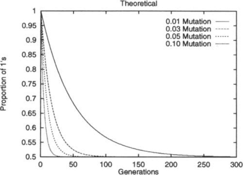
Assume that binary strings are being used (C = 2) and α = 1. Also assume the population is initially seeded only with l’s. Then the solution to the differential equation is:
p1(t)=e−2μt+12
which is very similar to the equation derived from physics for radioactive decay.
Figure 1 shows the decay curves derived via Equation 1 for different mutation rates. Although μ has no effect on the limiting distribution, increasing μ clearly increases the rate at which that distribution is approached. Although this result is quite intuitively obvious, the key point is that we can now make quantitative statements as to how the initial conditions and the mutation rate affect the speed of approaching equilibrium.
3 THE LIMITING DISTRIBUTION FOR RECOMBINATION
Geiringer’s Theorem (Geiringer 1944) describes the equilibrium distribution of an arbitrary population that is undergoing recombination, but no selection or mutation. To understand Geiringer’s Theorem, consider a population of ten strings of length four. In the initial population, five of the strings are “AAAA” while the other five are “BBBB”. If these strings are recombined repeatedly, eventually 24 strings will become equally likely in the population. In equilibrium, the probability of a particular string will approach the product of the initial probabilities of the individual alleles - thus asserting a condition of independence between alleles. Geiringer’s Theorem can be stated as follows:
Theorem 2
Let S be any string of L alleles: (a1,…, aL). If a population is recombined repeatedly (without selection or mutation) then:
limt→∞ps(t)=L∏i=1pai(0)
where pS(t) is the expected proportion of string S in the population at time t and pai(0)![]() is the proportion of allele a at locus (position) i in the initial population.
is the proportion of allele a at locus (position) i in the initial population.
Thus, the probability of string S is simply the product of the proportions of the individual alleles in the initial (t = 0) population. The equilibrium distribution illustrated in Theorem 2 is referred to as “Robbins’ equilibrium” (Robbins 1918). Theorem 2 holds for all standard recombination operators, such as n-point recombination and Po uniform recombination.2 It also holds for arbitrary cardinality alphabets. The key point is that recombination operators do not change the distribution of alleles at any locus; they merely shuffle those alleles at each locus.
3.1 OVERVIEW OF MARGINAL RECOMBINATION DISTRIBUTIONS
According to Booker (1992) and Christiansen (1989), the population dynamics of a population undergoing recombination (but no selection or mutation) is governed by marginal recombination distributions. To briefly summarize, ![]() A(B) is “the marginal probability of the recombination event in which one parent transmits the loci B ⊆ A and the other parent transmits the loci in AB” (Booker 1992). A and B are sets and AB represents set difference. For example, suppose one parent is xyz and the other is XYZ. Since there are three loci, A = {1, 2, 3}. Let B = {1, 2} and AB = {3}. This means that the two alleles xy are transmitted from the first parent, while the third allele Z is transmitted from the second parent, producing an offspring xyZ. The marginal distribution is defined by the probability terms
A(B) is “the marginal probability of the recombination event in which one parent transmits the loci B ⊆ A and the other parent transmits the loci in AB” (Booker 1992). A and B are sets and AB represents set difference. For example, suppose one parent is xyz and the other is XYZ. Since there are three loci, A = {1, 2, 3}. Let B = {1, 2} and AB = {3}. This means that the two alleles xy are transmitted from the first parent, while the third allele Z is transmitted from the second parent, producing an offspring xyZ. The marginal distribution is defined by the probability terms ![]() A(B), B ⊆ A. Clearly ∑B⊆AℛA(B)=1
A(B), B ⊆ A. Clearly ∑B⊆AℛA(B)=1![]() and under Mendelian segregation,
and under Mendelian segregation, ![]() A(B) =
A(B) = ![]() A(AB). In terms of the more traditional schema analysis, the set A designates the defining loci of a schema. Thus, the terms
A(AB). In terms of the more traditional schema analysis, the set A designates the defining loci of a schema. Thus, the terms ![]() A (A) =
A (A) = ![]() A (∅) refer to the survival of the schema at the defining loci specified by A.
A (∅) refer to the survival of the schema at the defining loci specified by A.
3.2 THE RATE AT WHICH ROBBINS’ EQUILIBRIUM IS APPROACHED
As stated earlier, Booker (1992) has suggested that the rate at which the population approaches Robbins’ equilibrium is the significant distinguishing characterization of different recombination operators. According to Booker, “a useful quantity for studying this property is the coefficient of linkage disequilibrium, which measures the deviation of current chromosome frequencies from their equilibrium levels”. Such an analysis has been performed by Christiansen (1989), but given its roots in mathematical genetics the analysis is not explicitly tied to more conventional analyses in the EA community. The intuitive hypothesis is that those recombination operators that are more disruptive should drive the population to equilibrium more quickly (see Mühlenbein (1998) for empirical evidence to support this hypothesis). Christiansen (1989) provides theoretical support for this hypothesis by stating that the eigenvalues for convergence are given by the ![]() A(A) terms in the marginal distributions. The smaller
A(A) terms in the marginal distributions. The smaller ![]() A(A) is, the more quickly equilibrium is reached, in the limit. Since disruption is the opposite of survival, the direct implication is that equilibrium is reached more quickly when a recombination operator is more disruptive.
A(A) is, the more quickly equilibrium is reached, in the limit. Since disruption is the opposite of survival, the direct implication is that equilibrium is reached more quickly when a recombination operator is more disruptive.
One very important caveat, however, is that this theoretical analysis holds only in the limit of large time, or when the population is near equilibrium. As GA practitioners we are far more interested in the short-term transient behavior of the population dynamics. Although equilibrium behavior can be studied by use of the margined probabilities ![]() A(A), studying the transient behavior requires all of the marginals
A(A), studying the transient behavior requires all of the marginals ![]() A(B), B ⊆ A. The primary goal of this section is to tie the marginal probabilities to the more traditional schema analyses, in order to analyze the complete (transient and equilibrium) behavior of a population undergoing recombination. The focus will be on recombination operators that are commonly used in the GA community: n-point recombination and Po uniform recombination. Several related questions will be addressed. For example, lowering Po from 0.5 makes Po uniform recombination less disruptive (
A(B), B ⊆ A. The primary goal of this section is to tie the marginal probabilities to the more traditional schema analyses, in order to analyze the complete (transient and equilibrium) behavior of a population undergoing recombination. The focus will be on recombination operators that are commonly used in the GA community: n-point recombination and Po uniform recombination. Several related questions will be addressed. For example, lowering Po from 0.5 makes Po uniform recombination less disruptive (![]() A(A) increases). How do the remainder of the marginals change? Can we compare n-point recombination and Po uniform recombination in terms of the population dynamics? Finally, what can we say about the transient dynamics? Although these questions can often only be answered in restricted situations the picture that emerges is that traditional schema analyses such as schema disruption and construction (Spears and De Jong 1998) do in fact yield important information concerning the dynamics of a population undergoing recombination.
A(A) increases). How do the remainder of the marginals change? Can we compare n-point recombination and Po uniform recombination in terms of the population dynamics? Finally, what can we say about the transient dynamics? Although these questions can often only be answered in restricted situations the picture that emerges is that traditional schema analyses such as schema disruption and construction (Spears and De Jong 1998) do in fact yield important information concerning the dynamics of a population undergoing recombination.
3.3 THE FRAMEWORK
The framework used in this section consists of a set of differential equations that describe the expected time evolution of the strings in a population of finite size (equivalently this can be considered to be the evolution of an infinite-size population). The treatment will hold for hyperplanes (schemata) as well, so the term “hyperplane” and “string” can be used interchangeably.
Consider having a population of strings. Each generation, pairs of strings (parents) are repeatedly chosen uniformly randomly for recombination, producing offspring for the next generation. Let Sh, Si, and Sj be strings of length L (alternatively, they can be considered to be hyperplanes of order L). Let psi (t) be the proportion of string Si at time t. The time evolution of Si will again involve terms of loss (death) and gain (birth). A loss will occur if parent Si is recombined with another parent such that neither offspring is S,. A gain will occur if two parents that are not Si are recombined to produce Si. Thus the following differential equation can be written for each string Si:
dpsi(t)d=−lossSi(t)+gainSi(t)
![]()
The losses can occur if Si is recombined with another string Sj such that Si and Sj differ by ∆(Si, Sj) ≡ k alleles, where k ranges from two to L. For example the string “AAAA” can (potentially) be lost if recombined with “AABB” (where k = 2). If Si and Sj differ by one or zero alleles, there will be no change in the proportion of string Si. In general, the expected loss for string Si at time t is:
lossSi(t)=∑SjpSi(t)Pd(Hk)where2≤Δ(Si,Sj)≡k≤L
The product pSi(t) pSj(t) is the probability that Si will be recombined with Sj, and Pd(Hk) is the probability that neither offspring will be Si. Equivalently, Pd(Hk) refers to the probability of disrupting the kth-order hyperplane Hk defined by the k different alleles. This is identical to the probability of disruption sis defined by De Jong and Spears (1992).
Gains can occur if two strings Sh, and Sj of length L can be recombined to construct Si. It is assumed that neither Sh or Sj is the same as Si at all defining positions (because then there would be no gain) and that either Sh or Sj has the correct allele for Si at every locus. Suppose that Sh and Sj differ at ∆(Sh, Sj) = k alleles. Once again k must range from two to L. For example, the string “AAAA” can (potentially) be constructed from the two strings “AABB” and “ABAA” (where k = 3). If Sh and Sj differ by one or zero alleles, then either Sh or Sj is equivalent to Si and there is no true construction (or gain).
Of the k differing alleles, m are at string Sh and n = k – m are at string Sj. Thus what is happening is that two non-overlapping, lower-order building blocks Hm and Hn are being constructed to form Hk (and thus the string Si). In general, the expected gain for string Si at time t is:
gainSi(t)=∑Sh,SjpSh(t)pSj(t)Pc(Hk|HmΛHn)where2≤Δ(Sh,Sj)≡k≤L

The product psh(t) pSj(t) is the probability that Sh will be recombined with Sj, and Pc(Hk | Hm ∧ Hn) is the probability that an offspring will be Si. Equivalently, Pc(Hk Hm![]() Hn) is the probability of constructing the kth-order hyperplane Hk (and hence string Si) from the two strings Sh and Sj that contain the non-overlapping, lower-order building blocks Hm and Hn. This is identical to the probability of construction as defined by Spears and De Jong (1998).
Hn) is the probability of constructing the kth-order hyperplane Hk (and hence string Si) from the two strings Sh and Sj that contain the non-overlapping, lower-order building blocks Hm and Hn. This is identical to the probability of construction as defined by Spears and De Jong (1998).
If the cardinality of the alphabet is C then there are CL different strings. This results in a system of CL simultaneous first-order differential equations. What is important to note is the explicit connection between Equations 2–3 and the more traditional schema theory for recombination, as exemplified by the probability of disruption Pd(Hk) and the probability of construction Pc(Hk Hm ∧ Hn).
3.4 TRADITIONAL SCHEMA THEORY AND THE MARGINALS
We are now in a position to also explain the link between the traditional schema theory and the marginal probabilities. Consider the prior example, where the recombination of the parents xyz and XYZ produced an offspring xyZ. The other offspring produced is XYz. This occurs if B = {1, 2} and AB = {3} or in the complementary situation where B = {3} and AB = {1, 2}. Hence, as pointed out earlier, ![]() A(B) =
A(B) = ![]() A (AB). However, this is identical to the situation in which the third-order hyperplane Hz = xyZ is constructed from the first-order hyperplane H1 = ##Z and the second-order hyperplane H2 = xy#.3 If we use |•| to denote the cardinality of a set, we can explicitly tie the probability of construction with the marginal probabilities:
A (AB). However, this is identical to the situation in which the third-order hyperplane Hz = xyZ is constructed from the first-order hyperplane H1 = ##Z and the second-order hyperplane H2 = xy#.3 If we use |•| to denote the cardinality of a set, we can explicitly tie the probability of construction with the marginal probabilities:
Pc(H|A||H|B|∧H|AB|)=ℛA(B)+ℛA(AB)=2ℛA(B)
where a hyperplane of order k = |A| is being constructed from lower-order hyperplanes of order m = |B| and order n = |AB|. Interestingly, Equation 4 allows us to correct an error in Booker (1992), where he computes the marginal distribution for Po uniform recombination. The marginal distribution should be:
ℛA(B)=[P0|B|(1−P0)|AB|+P0|AB|(1−P0)|B|]/2
.
Survival is a special form of construction in which one of the lower-order hyperplanes has zero order. Since disruption is the opposite of survival we can write:
Pd(H|A|)≡1−Pc(H|A||H|∅|∧H|A∅|)=1−2ℛA(A)
![]()
As mentioned earlier, according to Christiansen (1989), the smaller ![]() A(A) is, the more quickly equilibrium is reached in the limit. We can now connect this result to the concepts of disruption and construction in the framework given by Equations 2 – 3. If some hyperplane is above the equilibrium proportion then the loss terms will be more important, as they drive the hyperplane down to equilibrium. A decrease in
A(A) is, the more quickly equilibrium is reached in the limit. We can now connect this result to the concepts of disruption and construction in the framework given by Equations 2 – 3. If some hyperplane is above the equilibrium proportion then the loss terms will be more important, as they drive the hyperplane down to equilibrium. A decrease in ![]() A(A) indicates that a recombination operator is more disruptive. This increases the loss terms and drives the hyperplane down towards equilibrium more quickly. Likewise, if some hyperplane is below the equilibrium proportion then the gain terms will be more important, as they drive the hyperplane up towards equilibrium. Since marginals must sum to one, if
A(A) indicates that a recombination operator is more disruptive. This increases the loss terms and drives the hyperplane down towards equilibrium more quickly. Likewise, if some hyperplane is below the equilibrium proportion then the gain terms will be more important, as they drive the hyperplane up towards equilibrium. Since marginals must sum to one, if ![]() A(A) decreases some (or all) of the other marginals will increase to compensate. Thus, on the average a more disruptive recombination operator will increase the Pc(Hk |Hm ∧ Hn) terms and hence drive that hyperplane to equilibrium more quickly.
A(A) decreases some (or all) of the other marginals will increase to compensate. Thus, on the average a more disruptive recombination operator will increase the Pc(Hk |Hm ∧ Hn) terms and hence drive that hyperplane to equilibrium more quickly.
However, as stated before, the caveat lies in the phrase “in the limit”. Although a reduction in ![]() A(A) increases the other marginals on the average, there are situations where some marginals increase while others decrease. This can cause quite interesting transient behavior. The major contributor to this phenomena appears to be the order of the hyperplane, which we investigate in the following subsections.
A(A) increases the other marginals on the average, there are situations where some marginals increase while others decrease. This can cause quite interesting transient behavior. The major contributor to this phenomena appears to be the order of the hyperplane, which we investigate in the following subsections.
3.5 SECOND-ORDER HYPERPLANES
We first consider the case of second-order hyperplanes, which axe easiest to analyze. Consider the situation where the cardinality of the alphabet C = 2. In this situation there are four hyperplanes of interest: (#0#0#, #0#1#, #1#0#, #1#1#).4 Then the four differential equations describing the expected time evolution of these hyperplanes are:
dp00(t)dt=−poo(t)p11(t)Pd(H2)+p01(t)p10(t)Pc(H2|H1∧H1)dp00(t)dt=−po1(t)p10(t)Pd(H2)+p00(t)p11(t)Pc(H2|H1∧H1)dp10(t)dt=−po1(t)p10(t)Pd(H2)+p00(t)p11(t)Pc(H2|H1∧H1)dp11(t)dt=−poo(t)p11(t)Pd(H2)+p01(t)p10(t)Pc(H2|H1∧H1)
Thus for this special case the loss and gain terms axe controlled fully by one computation of disruption and one computation of construction. If two recombination operators have precisely the same disruption and construction behavior on second-order hyperplanes, the system of differential equations will be the same, and the time evolution of the system will be the same. This is true regardless of the initial conditions of the system.
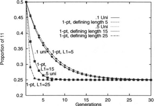
For example, consider one-point recombination and P0 uniform recombination. Suppose the defining length of the second-order hyperplane is L1. Then, Pd(H2) = L1/L for one-point recombination, and Pd(H2) = 2Po(l – P0) for uniform recombination. The computations for Pc(H2 | H1 ![]() H1) equal Pd(H2) for one-point and uniform recombination. Thus, one-point recombination should act the same as uniform recombination when the defining length L1 = 2 L Po(l – P0).
H1) equal Pd(H2) for one-point and uniform recombination. Thus, one-point recombination should act the same as uniform recombination when the defining length L1 = 2 L Po(l – P0).
To illustrate this, an experiment was performed in which a population of binary strings was initialized so that 50% of the strings were all 1’s, while 50% were all 0’s. The strings were of length L = 30 and were repeatedly recombined, generation by generation, while the percentage of the second-order hyperplane #1#1# was monitored. When Robbins’ equilibrium is reached the percentage of any of the four hyperplanes should be 25%. The experiment was run with 0.1 and 0.5 uniform recombination. Under those settings of Po, the theory indicates that one-point recombination should perform identically when the second-order hyperplanes have defining length 5.4 and 15, respectively. Since an actual defining length must be an integer, the hyperplanes of defining length 5 and 15 were monitored.
Figure 2 graphs the results.5 As expected, the results show a perfect match when comparing the evolution of H2 under 0.5 uniform recombination and one-point recombination when L1 = 15 (the two curves coincide almost exactly on the graph). The agreement is almost perfect when comparing 0.1 uniform recombination and one-point recombination when L1 = 5, and the small amount of error is due to the fact that the defining length had to be rounded to an integer. As an added comparison, the second-order hyperplanes of defining length 25 were also monitored. In this situation one-point recombination should drive these hyperplanes to equilibrium even faster than 0.5 uniform recombination (because one-point recombination is more disruptive in this situation). The graph confirms this observation.
It is important to note that the above analysis holds even for arbitrary cardinality alphabets C, although it was demonstrated for C = 2. The system of differential equations would have more equations and terms as C increases, but the computations would still only involve one computation of Pd(H2) and Pc(H2 | H1 ![]() H1), and those computations would be precisely the same. To see this, consider having C = 3, with an alphabet of {0, 1, 2}. Then #0#0# can be disrupted if recombined with #1#1#, #1#2#, #2#1#, or #2#2#. The probability of disruption is the same sis it was above. Similarly it can be shown that the probability of construction is the same as it was above.
H1), and those computations would be precisely the same. To see this, consider having C = 3, with an alphabet of {0, 1, 2}. Then #0#0# can be disrupted if recombined with #1#1#, #1#2#, #2#1#, or #2#2#. The probability of disruption is the same sis it was above. Similarly it can be shown that the probability of construction is the same as it was above.
3.5.1 The Rate of Decay for Second-Order Hyperplanes
It is interesting to note that, as with mutation, the decay of the curves in Figure 2 appears to be exponential in nature. This turns out to be true. To prove this, let us reconsider the differential equation describing the change in the expected proportion of the second-order hyperplane #1#1# at time t:
dp11(t)dt=−p00(t)p11(t)Pd(H2)+p01(t)p10(t)Pc(H2|H1∧H1)

In this case we know that Pd(H2) = Pc(H2 | H1 ![]() H1), so the equation can be simplified to:
H1), so the equation can be simplified to:
dp11(t)dt=Pd(H2)[p01(t)p10(t)−p00(t)p11(t)]

For the experiment leading to Figure 2 we also know that p01(t) = p10(t) and poo(t) = P11(t):
dp11(t)dt=Pd(H2)[p01(t)p01(t)−p11(t)p11(t)]
However, since p00(t)+p01(t)+p10(t)+ p11(t) = 1 it is easy to show that p01(t)=12−p11(t).![]() With some simplification this leads to:
With some simplification this leads to:
dp11(t)dt=Pd(H2)[14−p11(t)]
![]()
Given the initial condition that p11(0)=12![]() the solution to the differential equation is:
the solution to the differential equation is:
p11(t)=p00(t)=1+e−Pd(H2)t4
![]()
Similarly, it is easy to show that the proportions of the #0#1 # and #1#0# hyperplanes grow as follows (given the initial conditions that p01(0) = p10(0) = 0):
p11(t)=p00(t)=1−e−Pd(H2)t4
3.5.2 The Rate of Approaching Equilibrium
It is also possible to derive a more general result concerning the rate at which equilibrium is approached. To see this, consider Equation 5 again:
dp11(t)dt=Pd(H2)[p01(t)p10(t)−p00(t)p11(t)]
Let δ(t) = po1(t) p10(t) – p00(t) p11(t). Then it is very clear that
dp11(t)dt=dp00(t)dt=−dp01(t)dt=−dp10(t)dt=δ(t)Pd(H2)
Since δ(t) goes to zero as the proportions of all the second-order hyperplanes approach equilibrium, we can consider δ(t) to be a measure of linkage disequilibrium for second-order hyperplanes. We can now write:
dδ(t)dt=p01(t)dp10(t)dt+p10(t)dp01(t)dt−p00(t)dp11(t)dt−p11(t)dp00(t)dt

This simplifies to:
dδ(t)dt=−dp11(t)dt=−δ(t)Pd(H2)
The solution to this is simply:
δ(t)=−δ(0)e−Pd(H2)t
where δ(0) = p 01(0) p 10(0) – p 00(0) p11(0).
3.5.3 Summary of Second-Order Hyperplane Results
These results explicitly link traditional schema theory with the rate at which Robbins’ equilibrium is approached, for second-order hyperplanes. We have shown that for second-order hyperplanes, the time evolution of two different recombination operators can be compared simply by comparing their disruptive and constructive behavior. Two recombination operators will drive a second-order hyperplane to Robbins’ equilibrium at the same rate if their disruptive and constructive behavior are the same. It was also shown that δ(t), a measure of linkage disequilibrium for second-order hyperplanes, exponentially decays towards zero with the probability of disruption Pd(H2) being the rate of decay.
Unfortunately, similar results are harder to determine for higher-order hyperplanes, although some interesting results can be shown for Po uniform recombination, as shown in the following subsections.
3.6 UNIFORM RECOMBINATION AND LOW-ORDER HYPERPLANES
For P0 uniform recombination the loss and gain terms of Equations 2–3 are especially easy to compute. As stated earlier, losses can occur if an Lth-order hyperplane Si is recombined with an Lth-order hyperplane Sj such that Si and Sj differ by k alleles, where k ranges from two to L. But, according to De Jong and Spears (1992) this occurs with probability:
Pd(Hk)=1−P0k−(1−Po)k2≤k≤L
![]()
It can be shown that this is a unimodal function with a maximum at 0.5. Thus, the key point is that when the time evolution of the population undergoing recombination is expressed with CL differential equations, the effect of increasing or decreasing P0 from 0.5 reduces all of the loss terms in the differential equations, regardless of the order of the hyperplane. This slows the rate at which the equilibrium is approached.
Gains will occur if two hyperplanes Sh and Sj of order L can be recombined to construct Si. Again, suppose that Sh and Sj differ at k alleles, where k ranges from two to L. Of the k differing alleles, m are at hyperplane Sh and n = k – m are at hyperplane Sj. Then the probability of construction is:
Pc(Hk|Hm∧Hn)=P0m(1−P0)n+P0n(1−P0)m2≤k≤L,0<m<k
![]()
This has zero slope at Po = 0.5. The question now is under what conditions of n and m will Po = 0.5 represent a global (and the only) maximum. It is easy to show by counterexample that P0 = 0.5 is not a global maximum for arbitrary m and n (e.g., m = 1 and n = 4). However, there are various cases where Po = 0.5 is a global maximum - namely when m = 1 and n = 1, m = 1 and n = 2, m = 1 and n = 3, and when m = 2 and n = 2 (and the symmetric cases where m and n are interchanged). See Figure 3 for graphs of the probability of construction, as Po changes.
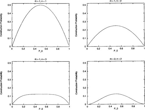
 Hn) for Po uniform recombination on second-order (m = 1, n = 1), third-order (m = 1, n = 2), and fourth-order hyperplanes (m = 1, n = 3 and m = 2, n = 2). The probability of construction monotonically decreases as Po is decreased/increased from 0.5.
Since we are interested in kth-order hyperplanes (where k = m + n), we have shown that for low-order hyperplanes (k < 5), construction is at a maximum when Po = 0.5 and construction decreases as Po decreases or increases from 0.5.
Thus, consider the time evolution of the hyperplanes in a population that are undergoing recombination, as modeled with the above differential equations. What we have shown is that if the hyperplanes have low order (k < 5), the effect of increasing or decreasing Po from 0.5 reduces all of the gain terms in the differential equations. Put in terms of the marginal probabilities we have shown that, for Po uniform recombination on low-order hyperplanes (fc < 5), increasing ![]() A(A) (moving Po from 0.5) will decrease all of the other marginals
A(A) (moving Po from 0.5) will decrease all of the other marginals ![]() A(B), ∅ ⊂ B ⊂ A. Given this, we can expect that reducing or increasing Po from 0.5 should monotonically decrease the rate at which the equilibrium is approached, even during the transient behavior of the system.
A(B), ∅ ⊂ B ⊂ A. Given this, we can expect that reducing or increasing Po from 0.5 should monotonically decrease the rate at which the equilibrium is approached, even during the transient behavior of the system.
To illustrate this, an experiment was performed in which a population of binary strings was initialized so that 50% of the strings were all l’s, while 50% were all 0’s. The strings were of length L = 30 and were repeatedly recombined, generation by generation, while the percentages of the fourth-order hyperplanes #1#1#1#1# and #0#1#1#1# were monitored. When Robbins’ equilibrium is reached the percentage of any of the fourth- order hyperplanes should be 6.25%. The experiment was run with uniform recombination, with Po ranging from 0.1 to 0.5 (higher values were ignored due to symmetry).
Figure 4 graphs the results. One can see that as Po increases to 0.5, the rate at which Robbins’ equilibrium is approached also increases, as expected. This holds even throughout the transient dynamics of the system.
3.7 UNIFORM RECOMBINATION AND HIGH-ORDER HYPERPLANES
It is natural to wonder how this extends to higher-order hyperplanes. Unfortunately, as pointed out above, there will be situations (of m and n) where Po = 0.5 does not represent a global maximum for construction. However, it is easy to prove that when m = n once again construction decreases as Po decreases or increases from 0.5. It appears as if this also holds for those situations where m and n are roughly equal (i.e., both axe roughly k/2), but eventually fails when m and n are sufficiently different (either m or n is close to 1). Figure 5 illustrates this for eighth-order hyperplanes. Although construction is maximized at Po = 0.5 when m = 4 and n = 4, this certainly isn’t true when m = 1 and n = 7. In fact, in that case construction is maximized when Po is roughly 0.13.
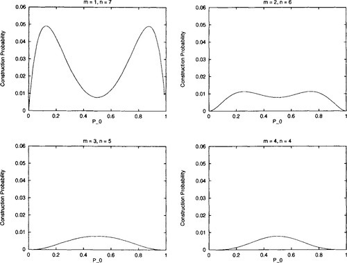 Hn) for Po uniform recombination, non eighth-order hyperplanes. The probability of construction does not always monotonically decrease as Po is decreased/increased from 0.5.
Put in terms of the marginal probabilities we have shown that, for Po uniform recombination on higher-order hyperplanes (k > 4), increasing ![]() A(A) (moving Po from 0.5) will decrease some (but not all) of the other marginals
A(A) (moving Po from 0.5) will decrease some (but not all) of the other marginals ![]() A(B), ∅ ⊂ B ⊂ A. Given this, we can expect that reducing or increasing Po from 0.5 should not necessarily monotonically decrease the rate at which the equilibrium is approached, during the transient behavior of the system.
A(B), ∅ ⊂ B ⊂ A. Given this, we can expect that reducing or increasing Po from 0.5 should not necessarily monotonically decrease the rate at which the equilibrium is approached, during the transient behavior of the system.
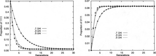
To illustrate this, an experiment was performed in which a population of binary strings was initialized so that 50% of the strings were all l’s, while 50% were all 0’s. The strings were of length L = 30 and were repeatedly recombined, generation by generation, while the percentages of the eighth-order hyperplanes #1#1#1#1#1#1#1#1# and #0#1#1#1#1#1#1#1# were monitored. When Robbins’ equilibrium is reached the percentage of any of the eighth-order hyperplanes should be approximately 0.39%. The experiment was run with uniform recombination, with Po ranging from 0.1 to 0.5 (higher values were ignored due to symmetry).
Figure 6 graphs the results, which are quite striking. Although the proportion of the hyperplane #1#1#1#1#1#1#1#1# decays smoothly towards its equilibrium proportion, this is certainly not true for the hyperplane #0#1#1#1#1#1#1#1#. Although Po = 0.5 uniform recombination does provide the fastest convergence in the limit of large time, as would be expected, it is also clear that Po = 0.1 provides much larger changes in the proportions during the early transient behavior. In fact, for all values of Po the change in the proportion of this hyperplane is so large that it temporarily overshoots the equilibrium proportion!
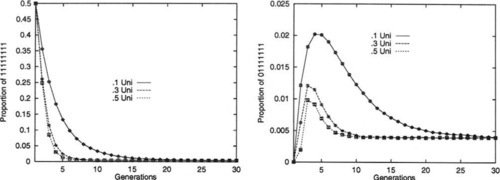
In summary, for higher-order hyperplanes, one can see that as Po increases to 0.5, the rate at which Robbins’ equilibrium is approached also increases, in the limit. However, this does not necessarily hold throughout the transient dynamics of the system. In fact, we have shown an example in which a less disruptive recombination operator provides more substantive changes in the early transient behavior.
4 THE LIMITING DISTRIBUTION FOR MUTATION AND RECOMBINATION
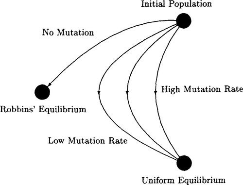
The previous sections have considered mutation and recombination in isolation. A population undergoing recombination approaches Robbins’ equilibrium, while a population undergoing mutation approaches a uniform equilibrium. What happens when both mutation and recombination act on a population? The answer is very simple. In general, Robbins’ equilibrium is not the same as the uniform equilibrium; hence the population can not approach both distributions in the long term. In fact, in the long term, the uniform equilibrium prevails and we can state a similar theorem for mutation and recombination.
Theorem 3
Let S be any string of L alleles: (a1, …, aL). If a population is mutated and recombined repeatedly (without selection) then:
limt→∞ps(t)=L∏i=11C

where ps(t) is the expected proportion of string S in the population at time t and C is the cardinality of the alphabet.
This is intuitively obvious. Recombination can not change the distribution of alleles at any locus – it merely shuffles alleles. Mutation, however, actually changes that distribution. Thus, the picture that arises is that a population that undergoes recombination and mutation attempts to approach a Robbins’ equilibrium that is itself approaching the uniform equilibrium. Put another way, Robbins’ equilibrium depends on the distribution of alleles in the initial population. This distribution is continually changed by mutation, until the uniform equilibrium distribution is reached. In that particular situation Robbins’ equilibrium is the same as the uniform equilibrium distribution. Thus the effect of mutation is to move Robbins’ equilibrium to the uniform equilibrium distribution. The speed of that movement will depend on the mutation rate μ (the greater that μ is the faster the movement). This is displayed pictorially in Figure 7.
5 SUMMARY
This paper investigated the limiting distributions of recombination and mutation, focusing not only on the dynamics near equilibrium, but also on the transient dynamics before equilibrium is reached. A population undergoing mutation approaches a uniform equilibrium in which every string is equally likely. The mutation rate μ and the initial population have no effect on that limiting distribution, but they do affect the transient behavior. The transient behavior was examined via a differential equation model of this process (which is analogous to radioactive decay in physics). This allowed us to make quantitative statements as to how the initial population, the cardinality C of the alphabet, and the mutation rate μ affect the speed at which the equilibrium is approached.
We then investigated recombination. A population undergoing only recombination will approach Robbins’ equilibrium. Geiringer’s Theorem indicates that this equilibrium distribution depends only on the distribution of alleles in the initial population. The form of recombination and the cardinality are irrelevant. The paper then attempted to characterize the transient behavior of the system, by developing a differential equation model of the population. Using this, it is possible to show that the probability of disruption (Pd) and the probability of construction (Pc) of schemata are crucial to the time evolution of the system. These probabilities can be obtained from traditional schema analyses. We also provide the connection between the traditional schema analyses and an alternative framework based on margined recombination distributions ![]() A(B) (Booker 1992). Survival (the opposite of disruption) is given by
A(B) (Booker 1992). Survival (the opposite of disruption) is given by ![]() A(A) while construction is given by the remaining marginals
A(A) while construction is given by the remaining marginals ![]() A(B), ∅ ⊂ B ⊂ A.
A(B), ∅ ⊂ B ⊂ A.
The analysis supports the theoretical result by Christiansen (1989) that, in the limit, more disruptive recombination operators (higher values of Pd or lower values of ![]() A(A) drive the population to equilibrium more quickly. However, we also show that the transient behavior can be subtle and can not be captured this simply. Instead the transient behavior depends on the whole probability distribution
A(A) drive the population to equilibrium more quickly. However, we also show that the transient behavior can be subtle and can not be captured this simply. Instead the transient behavior depends on the whole probability distribution ![]() A(B), B ⊆ A (and hence on the values of Pc).
A(B), B ⊆ A (and hence on the values of Pc).
The major contributor to interesting transient behavior appears to be the order of the hyperplane. We first examined second-order hyperplanes. By comparing one-point recombination and Po uniform recombination directly on second-order hyperplanes, we were able to derive a relationship showing when one-point recombination and uniform recombination both drive hyperplanes towards equilibrium at the same speed. We were also able to show that the linkage disequilibrium for second-order hyperplanes exponentially decays towards zero, with the probability of disruption Pd being the rate of decay. In these situations a more disruptive recombination operator drives hyperplanes towards equilibrium more quickly, even during the transient dynamics.
We then examined Po uniform recombination on hyperplanes of order k > 2. When k < 5 it is possible to show that when recombination becomes less disruptive (![]() A(A) increases), all of the remaining marginals
A(A) increases), all of the remaining marginals ![]() A(B) (∅ ⊂ B ⊂ A) decrease. Due to this, once again a more disruptive recombination operator drives hyperplanes towards equilibrium more quickly, even during the transient dynamics. However, when k > 4 the situation becomes much more interesting. In these situations some remaining marginals will decrease while others increase. This leads to behavior in which less disruptive recombination operators can in fact provide larger changes in hyperplane proportions, during the transient phase. These results are important because, due to the action of selection on a real GA population, the transient behavior of a population undergoing recombination is all that really matters.
A(B) (∅ ⊂ B ⊂ A) decrease. Due to this, once again a more disruptive recombination operator drives hyperplanes towards equilibrium more quickly, even during the transient dynamics. However, when k > 4 the situation becomes much more interesting. In these situations some remaining marginals will decrease while others increase. This leads to behavior in which less disruptive recombination operators can in fact provide larger changes in hyperplane proportions, during the transient phase. These results are important because, due to the action of selection on a real GA population, the transient behavior of a population undergoing recombination is all that really matters.
Finally, we investigated the joint behavior of a population undergoing both mutation and recombination. We showed that, in a sense, the behavior of mutation takes priority, in that mutation actually moves Robbins’ equilibrium until it is the same as the uniform equilibrium (i.e., all strings being equally likely).