
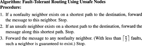
Fault-Tolerant Routing
Performance and fault tolerance are two dominant issues facing the design of interconnection networks for large-scale multiprocessor architectures. Fault tolerance is the ability of the network to function in the presence of component failures. However, techniques used to realize fault tolerance are often at the expense of considerable performance degradation. Conversely, making high-performance communication techniques resilient to network faults poses challenging problems. The presence of faults renders existing solutions to deadlock- and livelock-free routing ineffective. The result has been an evolution of techniques that must again address these basic issues in the presence of component failures.
Current-generation routers are very robust and do not appear to fail very often in practice. However, in some environments it is imperative that failures be anticipated and addressed, no matter how remote the possibility of component failures (e.g., mission-critical defense applications, space-borne systems, environmental controls, etc.). These operating environments are characterized by differing component failure rates, the ability for repair, and the feasibility of gracefully degraded operation. This has led to the development of a range of approaches to fault-tolerant routing in direct networks. This chapter presents a sampling of the various approaches with descriptions of specific routing algorithms. The ability to diagnose faults, particularly on-line, is a challenging problem and merits attention as a distinct research topic. The majority of techniques discussed in this chapter presume the existence of such diagnosis techniques and focus on how the availability of such diagnosis information can be used to develop robust and reliable communication mechanisms. A few routing algorithms combine diagnosis and routing. The difficulty of on-line diagnosis is a function of the switching technique.
This chapter first examines the effect of faults on current solutions to deadlock-free routing and establishes limits on the inherent redundancy of direct networks. This serves as the point of departure for the descriptions of the fault models and attendant routing algorithms.
6.1 Fault-Induced Deadlock and Livelock
It might initially appear that fully adaptive routing algorithms would enable messages to be routed around faulty regions. In reality, even the failure of a single link can destroy the deadlock freedom properties of adaptive routing algorithms. In this section, examples are presented to demonstrate how the occurrence of distinct classes of failures can lead to deadlock even for fully adaptive routing algorithms. Deadlocked configurations of messages are characterized, and key issues that must be resolved are identified. In the remainder of this chapter, fault-tolerant routing techniques are then presented and discussed according to how they have chosen to address these issues.
Consider Duato’s Protocol (DP), a fully adaptive, minimal-distance routing algorithm using wormhole switching in a 2-D mesh. This algorithm was shown in Figure 4.22. Recall that DP guarantees deadlock freedom by splitting each physical channel into two virtual channels: an adaptive channel and an escape channel. Fully adaptive routing is permitted using the adaptive channels, while deadlock is avoided by only permitting dimension-order routing on the escape channels.
Consider what happens when the router shown in Figure 6.1 fails. The figure shows three messages, A, B, and C. The destination nodes of these messages are also shown, although the source nodes are not. Note that the state shown in the figure is not dependent on the location of the source nodes. The figure illustrates the network state at the point in time where all messages have only the last dimension to traverse. Since DP is a minimal-distance routing algorithm, in this last dimension a message has only two candidate virtual channels, and both of them traverse the same physical channel. Suppose that message A reserved adaptive channels from node I to node J, and that message B reserved the escape channel at node I and then two vertical adaptive channels and two horizontal escape channels, reaching node J. It is apparent from the figure that message A can never make progress since the physical channel connected to the failed router is labeled faulty. Similarly, message B cannot make progress. In addition to blocking the messages requesting a faulty link, a faulty component can also block other messages. As can be seen in Figure 6.1, message C cannot make progress because the two virtual channels requested by it are occupied by messages A and B, respectively. Thus, the messages cannot advance and remain in an effectively deadlocked configuration even though cyclic dependencies between resources do not exist.
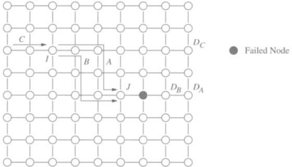
Figure 6.1 An example of the occurrence of deadlock due to faults in the presence of fully adaptive routing.
An equivalent situation can be constructed even if routers have multiple virtual channels and multiple virtual lanes in each channel. All lanes may be occupied by other messages. In general, if the fault is permanent, then any message waiting for the faulty component waits indefinitely, holding buffer and channel resources. The effect of the fault is propagated through permissible dependencies to affect messages that may not have to traverse the faulty component. These messages are said to form a wait chain [123]. Misrouting can avoid such deadlock, but must be controlled so that livelock is avoided and newly introduced dependencies do not produce deadlock. Fault recovery mechanisms must (1) recover messages indefinitely blocked on faulty components and (2) be propagated along wait chains to recover messages indirectly blocked on faulty components.
Pipelined switching mechanisms are particularly susceptible to faults due to the existence of dependencies across multiple routers. However, similar examples can be constructed with messages transmitted using packet switching or VCT switching. In this case, messages cannot make progress due to lack of buffer space in the next node along the path. Deadlock may be forestalled, but can eventually occur. While the above example portrays the effect of a static fault, dynamic faults can interrupt a message in progress and are more difficult to handle. Consider the failure of a link during the transmission of a data flit. Following data flits remain blocked in flit buffers with no routing information. These flits remain indefinitely in the network unless they are explicitly removed. Any other message that becomes blocked waiting for these buffers to become free starts the formation of a wait chain that can lead to deadlock.
From the above example, it is possible to identify several issues that must be addressed in the design of fault-tolerant routing algorithms.
1. If a header encounters a faulty component, messages must employ nonminimal routing. Misrouting must be controlled so that livelock is avoided and newly introduced dependencies do not produce deadlock among messages in the network. Typically this can be achieved with additional routing resources (e.g., virtual channels, packet buffers) and suitable routing restrictions among them. This is the minimum functionality required for tolerating static faults.
2. In the case of dynamic faults where message transmission is interrupted and message contents possibly corrupted by a component failure, recovery mechanisms must traverse and eliminate or prevent all wait chains. Otherwise it is possible that these messages will remain in the network indefinitely, occupying resources, and possibly lead to deadlock. Furthermore, some protocol is required either to recover the possibly corrupted message or to notify the source node so that a new copy of the message is transmitted.
As we might expect, solutions to these problems are dependent upon the type and pattern of the faulty components and the network topology. The next section shows how direct networks possess natural redundancy that can be exploited, by defining the redundancy level of the routing function. The remaining sections will demonstrate how the issues mentioned above are addressed in the context of distinct switching techniques.
6.2 Channel and Network Redundancy
This section presents a theoretical basis to answer a fundamental question regarding fault-tolerant routing in direct networks: What is the maximum number of simultaneous faulty channels tolerated by the routing algorithm? This question has been analyzed in [95] by defining the redundancy level of the routing function and proposing a necessary and sufficient condition to compute its value.
If a routing function tolerates f faulty channels, it must remain connected and deadlock-free for any number of faulty channels less than or equal to f. Note that, in addition to connectivity, deadlock freedom is also required. Otherwise, the network could reach a deadlocked configuration when some channels fail.
The following definitions are required to support the discussion of the behavior of fault-tolerant routing algorithms. In conjunction with the fault model, the following terminology can be used to discuss and compare fault-tolerant routing algorithms.
A routing algorithm is said to be f fault recoverable if, for any f failed components in the network, a message that is undeliverable will not hold network resources indefinitely. If a network is fault recoverable, the faults will not induce deadlock.
Ideally, we would like the network to be f fault tolerant for large values of f. Practically, however, we may be satisfied with a system that is f fault recoverable for large values of f and f1 fault tolerant for f1 ![]() f, so that only the functionality of a small part of the network suffers as a result of a failed component. Certainly, we want to avoid the situation where a few faults may cause a catastrophic failure of the entire network, or equivalently deadlocked configurations of messages. Finally, the next definition gives the redundancy level of the network.
f, so that only the functionality of a small part of the network suffers as a result of a failed component. Certainly, we want to avoid the situation where a few faults may cause a catastrophic failure of the entire network, or equivalently deadlocked configurations of messages. Finally, the next definition gives the redundancy level of the network.
Note that an algorithm has a redundancy level equal to r iff it is r fault tolerant and it is not r + 1 fault tolerant. The analysis of the redundancy level of the network is complex. Fortunately, there are some theoretical results that guarantee the absence of deadlock in the whole network by analyzing the behavior of the routing function R in a subset of channels C1 (see Section 3.1.3). Additionally, that behavior does not change when some channels not belonging to C1 are removed. That theory can be used to guarantee the absence of deadlock when some channels fail.
Suppose that there exists a routing subfunction R1 that satisfies the conditions of Theorem 3.1. Let C1 be the subset of channels supplied by R1. Now, let us consider the effects of removing some channels from the network. It is easy to see that removing channels not belonging to C1 does not add indirect dependencies between the channels belonging to C1. It may actually remove indirect dependencies. In fact, when all the channels not belonging to C1 are removed, there are no indirect dependencies between the channels belonging to C1. Therefore, removing channels not belonging to C1 does not introduce cycles in the extended channel dependency graph of R1. However, removing channels may disconnect the routing function. Fortunately, if a routing function is connected when it is restricted to use the channels in C1, it will remain connected when some channels not belonging to C1 are removed. Thus, if a routing function R satisfies the conditions proposed by Theorem 3.1, it will still satisfy them after removing some or all of the channels not belonging to C1. In other words, it will remain connected and deadlock-free. So, we can conclude that all the channels not belonging to C1 are redundant.
We can also reason in the opposite way. In general, there will exist several routing subfunctions satisfying the conditions proposed by Theorem 3.1. We will restrict our attention to the minimally connected routing subfunctions satisfying those conditions because they require a minimum number of channels to guarantee deadlock freedom. Let R1, R2, …, Rk be all the minimally connected routing subfunctions satisfying the conditions proposed by Theorem 3.1. Let C1, C2, …, Ck be the channel subsets supplied by those routing subfunctions. The set of redundant channels is given by
When C1 ∩ C2∩ … ∩Ck = ∅, all the channels are redundant. Consider again the channel subsets C1, C2, …, Ck. As the associated routing subfunctions are minimally connected, the failure of a single channel Cj ∈ Ci will prevent us from using Ci to prove that R is deadlock-free. If the subsets C1, C2, …, Ck were disjoint, the routing function R would have a redundancy level equal to k − 1. Effectively, the worst case occurs when each faulty channel belongs to a different subset. The failure of k − 1 channels will still allow us to use one channel subset to prove deadlock freedom. However, when a channel from each subset fails, we can no longer guarantee the absence of deadlock.
In general, the subsets C1, C2, …,Ck are not disjoint. In this case, the redundancy level will be less than k − 1. An example of channel subsets is shown in Figure 6.2. In order to compute the redundancy level of the network, it is only necessary to find the smallest set of channels Cm = {c1, c2, …, cr+1} such that at least one channel in Cm belongs to Ci, ∀i ∈ {1, 2, …,k}. If all the channels belonging to Cm fail, we cannot guarantee the absence of deadlock. Thus, the redundancy level is equal to the cardinality of Cm minus 1. This intuitive view is formalized by the following theorem:
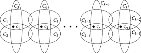
Figure 6.2 Channel sets supplied by all the minimally connected routing subfunctions of R and the corresponding elements in Cm.
Theorem 6.1 is only applicable to physical channels if they are not split into virtual channels. If virtual channels are used, the theorem is only valid for virtual channels. However, it can be easily extended to support the failure of physical channels by considering that all the virtual channels belonging to a faulty physical channel will become faulty at the same time. Theorem 6.1 is based on Theorem 3.1. Therefore, it is valid for the same switching techniques as Theorem 3.1, as long as edge buffers are used.
6.3 Fault Models
The structure of fault-tolerant routing algorithms is a natural consequence of the types of faults that can occur and our ability to diagnose them. The patterns of component failures and expectations about the behavior of processors and routers in the presence of these failures determines the approaches to achieve deadlock and livelock freedom. This information is captured in the fault model. The fault-tolerant computing literature is extensive and thorough in the definition of fault models for the treatment of faulty digital systems. In this section we will focus on common fault models that have been employed in the design of fault-tolerant routing algorithms for reliable interprocessor networks.
One of the first considerations is the level at which components are diagnosed as having failed. Typically, detection mechanisms are assumed to have identified one of two classes of faults. Either the entire processing element (PE) and its associated router can fail, or any communication channel may fail. The former is referred to as a node failure, and the latter as a link failure. On a node failure, all physical links incident on the failed node are also marked faulty at adjacent routers. When a physical link fails, all virtual channels on that particular physical link are marked faulty. Note that many types of failures will simply manifest themselves as link or node failures. For example, the failure of the link controller, or the virtual channel buffers, appears as a link failure. On the other hand, the failure of the router control unit or the associated PE effectively appears as a node failure. Even software errors in the messaging layer can lead to message handlers “locking up” the local interface and rendering the attached router inoperative, effectively resulting in a node fault. Hence, this failure model is not as restrictive as it may first appear.
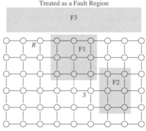
This model of individual link and node failures leads to patterns of failed components. Adjacent faulty links and faulty nodes are coalesced into fault regions. Generally, it is assumed that fault regions do not disconnect the network, since each connected network component can be treated as a distinct network. Constraints may now be placed on the structure of these fault regions. The most common constraint employed is that these regions be convex. As will become apparent in this chapter, concave regions present unique difficulties for fault-tolerant routing algorithms. Some examples of fault regions are illustrated in Figure 6.3. Convex regions may be further constrained to be block fault regions—regions whose shape is rectangular. This distinction is meaningful only in some topologies, whereas in other topologies, convex faults imply a block structure. Given a pattern of random faults in a multidimensional k-ary n-cube, rectangular fault regions can be constructed by marking some functioning nodes as faulty to fill out the fault regions.

This can be achieved in a fully distributed manner. The nodes are generally assumed to possess some ability for self-test as well as the ability to test neighboring nodes. We can envision an approach where, in one step, each node performs a self-test and interrogates the status of its neighbors. If neighbors or links in two or more dimensions are faulty, the node transitions to a faulty state, even though it may be nonfaulty. This diagnosis step is repeated. After a finite number of steps bounded by the diameter of the network, fault regions will have been created and will be rectangular in shape. In multidimensional meshes and tori under the block fault model, fault-free nodes are adjacent to at most one faulty node (i.e., along only one dimension). Note that single component faults correspond to the block fault model with block sizes of 1.
The block fault model is particularly well suited to evolving trends in packaging technology and the use of low-dimensional networks. We will continue to see subnetworks implemented in chips, multichip modules (MCMs), and boards. Failures within these components will produce block faults at the chip, board, and MCM level. Construction of block fault regions often naturally falls along chip, MCM, and board boundaries. For example, if submeshes are implemented on a chip, failure of two or more processors on a chip may result in marking the chip as faulty, leading to a block fault region comprised of all of the processors on the chip. The advantages in doing so include simpler solutions to deadlock- and livelock-free routing.
Failures may be either static or dynamic. Static failures are present in the network when the system is powered on. Dynamic failures appear at random during the operation of the system. Both types of faults are generally considered to be permanent; that is, they remain in the system until it is repaired. Alternatively, faults may be transient. As integrated circuit feature sizes continue to decrease and speeds continue to increase, problems arise with soft errors that are transient or dynamic in nature. The difficulty of designing for such faults is that they often cannot be reproduced. For example, soft errors that occur in flight tests of avionics hardware often cannot be reproduced on the ground. In addition, soft errors may become persistent, defying fault-tolerant schemes that rely on diagnosis of hard faults prior to system start-up. When dynamic or transient faults interrupt a message in progress, portions of messages may be left occupying message or flit buffers. Fault recovery schemes are necessary to remove such message components from the network to avoid deadlock, particularly if such messages have become corrupted and can no longer be routed (e.g., the message header has been altered or has already been forwarded).
In addition to how components fail, techniques can depend on when they fail. There are a broad range of operational environments characterized by distinct rates at which components may fail. These rates can be measured by the mean time between failures (MTBF). Moreover, the mean time to repair (MTTR) can vary significantly, from hours or days for laboratory-based machines to years of unattended operation for space-based systems. It is unlikely that one set of fault-tolerant routing techniques will be cost-effective or performance-effective across a large range of such systems. For example, we may have MTTR ![]() MTBF. In this case, the probability of the second or the third fault occurring before the first fault is repaired is very low. Therefore, the maximum number of faulty components at any given time is expected to be small (e.g., a maximum of two to three faulty nodes or associated links). The system may be expected to continue operating, although with degraded interprocessor communication performance, until the repair can be effected. Many commercial systems have been found to fit this characterization. For such relatively low fault rate environments, it may be feasible to employ lower-cost software-based approaches to handle the rerouting of messages that encounter faulty network components. Alternatively, for systems experiencing long periods of unattended operation such as space-borne systems (effectively MTTR → ∞), the number of concurrent failures can continue to grow. Thus, the attendant fault tolerance techniques must be more resilient, and more expensive custom solutions may be appropriate.
MTBF. In this case, the probability of the second or the third fault occurring before the first fault is repaired is very low. Therefore, the maximum number of faulty components at any given time is expected to be small (e.g., a maximum of two to three faulty nodes or associated links). The system may be expected to continue operating, although with degraded interprocessor communication performance, until the repair can be effected. Many commercial systems have been found to fit this characterization. For such relatively low fault rate environments, it may be feasible to employ lower-cost software-based approaches to handle the rerouting of messages that encounter faulty network components. Alternatively, for systems experiencing long periods of unattended operation such as space-borne systems (effectively MTTR → ∞), the number of concurrent failures can continue to grow. Thus, the attendant fault tolerance techniques must be more resilient, and more expensive custom solutions may be appropriate.
The behavior of failed components is also important, and the system implementation must preserve certain behaviors to ensure deadlock freedom. The failed node can no longer send or receive any messages and is effectively removed from the network. Otherwise messages destined for these nodes may block indefinitely, holding buffers and leading to deadlock. In the absence of global information about the location of faults, this behavior can be preserved in practice by having routers adjacent to a failed node remove from the network messages destined for the failed router. It is also generally assumed that the faults are nonmalicious. Malicious injection of faults is not inherently an issue to be addressed by routing algorithms, although malicious faults can lead to flooding of the network with messages. Solutions in the presence of malicious or Byzantine faults can become complicated and involve interpretation of the messages; they belong to higher-level protocol layers. This chapter is more concerned with routing messages around faulty components.
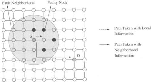
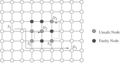
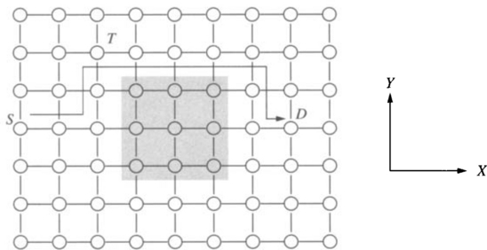
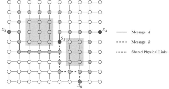
Finally, the fault model specifies the extent of the fault information that is available at a node. At one extreme, only the fault status of adjacent nodes is known. At the other extreme, the fault status of every node in the network is known. In the latter case, optimal routing decisions can be made at an intermediate node; that is, messages can be forwarded along the shortest feasible path in the presence of faults. However, in practice it is difficult to provide global updates of fault information in a timely manner without some form of hardware support. The occurrence of faults during this update period necessitates complex synchronization protocols. Furthermore, the increased storage and computation time for globally optimal routing decisions have a significant impact on performance. At the other extreme, fault information is limited to the status of adjacent nodes. With only local fault information, routing decisions are relatively simple and can be computed quickly. Also, updating the fault information of neighboring nodes can be performed simply. However, messages may be forwarded to a portion of the network with faulty components, ultimately leading to longer paths. In practice, routing algorithm design is typically a compromise between purely local and purely global fault status information. Figure 6.4 shows an example of the utility of having nonlocal fault information. The dashed line shows the path that would have been taken by a message from S to D. The solid line represents a path that the message could have been routed along had knowledge of the location of the faulty nodes been made available at the source. Finally, information aggregated at a node may be more than a simple list of faulty links and nodes in the network or local neighborhood. For example, status information at a node may indicate the existence of a path(s) to all nodes at a distance of k links. Such a representation of node status implicitly encodes the location and distribution of faults. This is in contrast to an explicit list of faulty nodes or links within a k-neighborhood. Computation of such properties is a global operation, and we must be concerned about handling faults during that computation interval.
Developing algorithms for acquiring and maintaining fault information within a neighborhood is the problem of fault diagnosis. This is an important problem since diagnosis algorithms executing on-line consume network bandwidth and must provide timely updates to be useful. The notions of diagnosis within network fault models have been formalized in [27, 28]. In k-neighborhood diagnosis, each node records the status of all faulty nodes within distance k. In practice it may not be possible to determine the status of all nodes within distance k since some nodes may be unreachable due to faults. This leads to the less restrictive notion of k-reachability diagnosis [28]. In this case, each nonfaulty node can determine the status of each faulty node within distance k that is reachable via nonfaulty nodes. Algorithms for diagnosis are a function of the type of faults; dynamic fault environments will result in diagnosis algorithms different from those that occur in static fault environments.
In summary, the power and flexibility of fault-tolerant routing algorithms are heavily influenced by the characteristics of the fault model. The model in turn specifies alternatives for one or more attributes as discussed in this section. Examples are provided in Table 6.1.
Table 6.1
Examples of fault-tolerant model attributes.
| Attribute | Options |
| Failure type | Node, physical or virtual link |
| Fault region | Block, convex, concave, random |
| Failure mode | Static, dynamic, transient |
| Failure time | MTTR, MTBF |
| Behavior of faulty components | Inoperable, receive, transmit |
| Fault neighborhood | Local, global, k-neighborhood, encoded |
6.4 Fault-Tolerant Routing in SAF and VCT Networks
This section describes several useful paradigms for rerouting message packets in the presence of faulty network components. In SAF and VCT networks the issue of deadlock avoidance becomes one of buffer management. Packets cannot make forward progress if there are no buffers available at an adjacent router. Unless otherwise stated, the techniques described in this section generally address the issue of rerouting around faulty components under the assumption that the issue of deadlock freedom is guaranteed by appropriate buffer management techniques such as those described in Chapter 4. Rerouting around faulty components necessitates nonminimal routing, and therefore the routing algorithms must ensure that livelock is avoided.
The early research on fault-tolerant routing in SAF and VCT networks largely focused on high-dimensional networks such as the binary hypercube topology. This was in part due to the dependence of message latency on distance and the low average internode distance in such topologies. Additional benefits included low diameter, logarithmic number of ports per router, and an interconnection structure that matched the communication topology of many parallel algorithms. In principle, the techniques developed for binary hypercubes can be suitably extended to the more general k-ary n-cube and often the multidimensional mesh topologies.
In multidimensional direct networks, if the number of faulty components is less than the degree of a node, then the features of the topology can be exploited to find a path between any two nodes. For example, consider an n-dimensional binary hypercube with f <n faulty components. In this topology there are n disjoint paths of length no greater than n + 2 between any pair of nodes [300]. As a result, n − 1 faulty components cannot physically disconnect the network, and we expect to be able to describe an (n − 1) fault-tolerant routing algorithm. The behavior of these algorithms is sensitive to the extent of the fault information available at an intermediate node. If the fault status of larger regions around the intermediate node is known, more informed routing decisions can be made with consequent improved performance. If only local information is available, routing decisions are fast and adjacent faulty regions can be avoided. However, the lack of any lookahead prevents choosing globally efficient routes, and path lengths may be longer than necessary. The following routing algorithms differ in the manner in which global information about the location and distribution of faulty components is acquired and used.
6.4.1 Routing Algorithms Based on Local Information
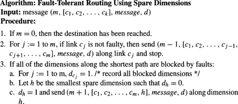
Faulty components can be sidestepped by traversing a dimension orthogonal to the dimensions leading to the faulty components. Chen and Shin [53] describe such an algorithm for routing in binary hypercubes. Unlike k-ary n-cubes, messages in binary hypercubes (k = 2) need only traverse one link in each dimension (refer to the description in Chapter 1). If the source and destination node addresses differ in m bits, then the message will traverse m dimensions on a shortest path from the source to the destination. This sequence of dimensions is specified as a coordinate sequence and is represented as a list of dimensions. At an intermediate node, a dimension that is not on the shortest path to the destination is referred to as a spare dimension. When all of the shortest paths toward the destination from an intermediate node are blocked by faults, the message is transmitted across a spare dimension. The dimensions that were blocked by a fault, as well as those used as a spare dimension, are recorded in an n-bit tag maintained in the message header. Note that the size of the tag accommodates at most n − 1 faulty components. The resulting message is comprised of several components: (m, [c1, c2, …,ck], message, d). The value of m represents the distance to the destination. When m = 0, the router can assert that the local PE is the destination. The tag d is initialized to zero at the source. When an intermediate node receives a message, it is forwarded along one of the dimensions in the coordinate sequence. The header is updated to decrement m and eliminate the dimension being traversed from the coordinate sequence. When blocked by faults along all of the shortest paths, the value of m is incremented, the spare dimension is added to the coordinate sequence, the tag d is updated, and the new message is misrouted along the spare dimension. This approach is (n − 1) fault tolerant. The routing algorithm is described in Figure 6.5.
In [53], the algorithm is shown to be able to route messages between any two nodes if the number of faulty components is less than n. In this case there is at least one spare dimension into the node that is nonfaulty, and the algorithm will find that spare dimension. This approach works well in high-dimensional networks. While the algorithm relies on purely local fault information, it can be extended to propagate fault information to nonneighboring nodes and to use this information effectively. Details can be found in [53].
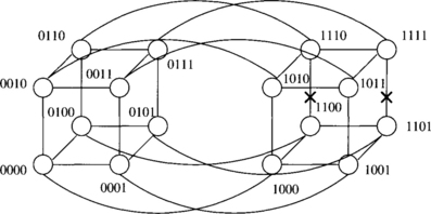
Consider the example of a message being routed from node 0010 to node 1101 in Figure 6.6. The original message is (4, [3, 2, 1, 0], message, 0000). The execution of the routing algorithm at the source sends the message with header (3, [2, 1, 0], message, 0000) to node 1010. This node sends (2, [1, 0], message, 0000) to node 1110. At this point a fault on the next smaller dimension causes the message (1, [1], message, 0000) to be forwarded to node 1111. The message must now be misrouted since the only path to the destination is blocked by a fault. The bit in the tag corresponding to this dimension is set, as well as the lowest available spare dimension. The message (2, [1, 0], message, 0011) is sent to node 1110, where it is again routed back to node 1111 as (1, [1], message, 0011). This is due to the fact that no record of the previous traversal is maintained in the header. However, now at node 1111 dimension 2 is picked as the spare dimension since the tag value is 0011, in effect retaining some history information. The message (2, [1, 2], message, 0111) is routed to node 1011, where it can now be routed to node 1101 via dimension 1 and then dimension 2.
The preceding approach relies on a fixed number of failures to guarantee message delivery, although the probability of delivery with values of f > n is shown to be very high [53]. An alternative to deterministic approaches is the use of randomization to produce probabilistically livelock-free, nonminimal, fault-tolerant routing algorithms. The intuition behind the use of randomization is that repetitive sequences of link traversals typical of livelocked messages are avoided with a high probability. The thesis is that this can be achieved without the higher overhead costs in header size and routing decision logic of deterministic approaches to livelock freedom.
The Chaos router incorporates randomization to produce a nonminimal fault-tolerant routing algorithm using VCT switching. The use of VCT switching in conjunction with nonminimal routing and randomization is proposed as a means to produce very high-speed, reliable communication substrates [187, 188, 189]. In chaotic routing, messages are normally routed along any profitable output channel. When a message resides in an input buffer for too long, blocked by busy output buffers, it is removed from the input buffer and stored in a local buffer pool. Messages in the local buffer pool are given a higher priority when output buffers become free, and messages from this pool are periodically reinjected into the network. In principle, if we have infinite storage at a node, removal of messages after a timeout breaks any cyclic dependencies and therefore prevents deadlock. In reality, the size of the buffer pool at a node is finite and is implemented as a queue. When this queue is full and a message must be stored in the queue, a random message is selected and misrouted. This is sufficient to prevent deadlock. However, livelock is still a source of concern. The key idea here is that a message has a nonzero probability of avoiding misrouting. This is in contrast to deterministic approaches, where given a specific router state, one fixed message is always selected for misrouting. The analysis of chaotic routing shows that the probability of infinite length paths approaches 0. Thus if a link is faulty, all messages using that link will be forwarded along other profitable links or misrouted around the faulty region.
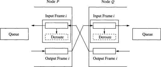
Figure 6.7 provides a simplified illustration of the operation of a channel along a dimension using chaos routing. Each channel supports one input frame and one output frame to an adjacent router. Messages appearing in the input frames can be routed along any free profitable output dimension if the corresponding output frame is free. If the message in the input frame cannot be forwarded, then it is stored in the local queue. If the queue is full, then a random message must be removed from the queue and misrouted. In this case, some output frame must be guaranteed to become free. The deroute buffers associated with the input frames ensure that this is indeed the case. This works as follows. When the message in input frame i in node P cannot be forwarded and the queue is full, that message is moved to the associated deroute buffer. We know that by freeing an input frame along channel i, node P can receive a message from node Q. This permits progress in node Q’s queue, and therefore the input frame i in node Q can be emptied. Consequently, the output frame i in node P can be emptied and can accommodate a message from the queue, and the rerouted message in the deroute buffer i can find its way into the queue. An alternative view toward understanding chaotic routing is to note that all six buffers across a dimension (e.g., as shown in Figure 6.7) cannot be occupied by messages concurrently. If dimensions are served in a round-robin manner, then one output frame will eventually become free, permitting movement of messages from the queue to output frames, and therefore from input frames to output frames or the queue. Finally, we note that whenever an output frame becomes free, messages in the queue have priority over messages in the input frame. This exchange protocol across the channel guarantees deadlock freedom. A detailed description of the Chaos router can be found in Chapter 7.
If an adjacent channel is diagnosed or inferred as being faulty, the corresponding output frame will not empty. This frame is effectively unavailable, and packets attempting to use this channel are naturally rerouted. There is the problem of recovering the packet that is in the output frame at the time the adjacent router has been diagnosed as faulty. Subsequent efforts have focused on augmenting the natural fault tolerance of chaotic routing with more efficient schemes that avoid losing a packet [356].
6.4.2 Routing Algorithms Based on Nonlocal Information
The preceding approaches assumed the availability of only local information with respect to faulty components—neighboring links and nodes. The greater the extent of the fault information that is available at a node, the more efficient routing decisions can be. Assume that each node has a list of faulty links and nodes within a k-neighborhood [198], that is, all faulty components within a distance of k links. The preceding routing algorithm might be modified as follows. Consider an intermediate node X = (xn–1, xn–2, …,x1, x0) that receives a message with a coordinate sequence (c1, c2, …, cr) that describes the remaining sequence of dimensions to be traversed to the destination. From the coordinate sequence we can construct the addresses of all nodes on a minimum-length path to the destination. For example, from intermediate node 0110, the coordinate sequence (0, 2, 3) describes a path through nodes 0111, 0011, and 1011. By examining all possible r! orderings of the coordinate sequence, we can generate all paths to the destination. If the first k elements of any such path are nonfaulty, the message can be forwarded along this path. The complexity of this operation can be reduced by examining only the r disjoint paths to the destination. These disjoint paths correspond to the following coordinate sequences: (c1, c2, …, cr), (c2, c3, …, cr, c1), (c3, c4, …, cr, c1, c2), and so on.
Rather than explicitly maintaining a list of faulty components in a k-neighborhood, an alternative method for expanding the extent of fault information is by encoding the state of a node. Lee and Hayes [198] introduced the notion of unsafe node. A nonfaulty node is unsafe if it is adjacent to two or more faulty or unsafe nodes. Each node now maintains two lists: one of faulty adjacent nodes and one for unsafe adjacent nodes. With a fixed set of faulty components, the status of a node may be faulty, nonfaulty, or unsafe. The status can be computed for all nodes in parallel in O(log3 N) steps for N nodes. Each node examines the state of its neighbors and changes its state if two or more are unsafe/faulty. A node need only transmit state information to the neighboring nodes if the local state has changed. This labeling algorithm will produce rectangular regions of nodes marked as faulty or unsafe. Figure 6.8 shows an example of the result of the labeling process in a 2-D mesh.
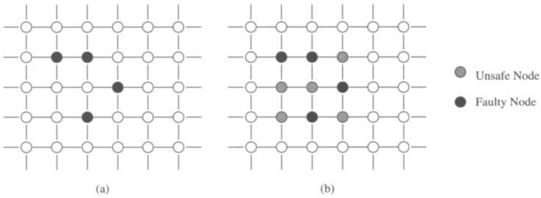
Figure 6.8 An example of the unsafe node designation: (a) faulty nodes and (b) nodes labeled as unsafe.
With fault distributions encoded in the state of the nodes, the approach toward routing now can be further modified. The unsafe status of nodes serves as a warning that messages may become trapped or delayed if routed via these nodes. Therefore, the routing algorithm is structured to first route a message to an adjacent nonfaulty node on a shortest path to the destination. If such a node does not exist, the message is routed to an unsafe node on a shortest path to the destination. If no such neighboring node can be found, then the message is misrouted to any adjacent nonfaulty node. By construction, in binary hypercubes every nonfaulty and unsafe node must be connected to at least one nonfaulty node if the number of faulty components is less than ![]() . This is not necessarily true for lower-dimensional networks such as meshes, as shown in Figure 6.9. This algorithm is summarized in Figure 6.10. In this paradigm, since functioning nodes can be labeled as unsafe, messages may originate from or be destined to unsafe nodes. Step 2 of the algorithm ensures that such messages can be delivered. The overall structure of the algorithm is such that paths are generally constructed through fault-free nodes and around regions of unsafe and faulty nodes. An example of such routing around the rectangular fault regions that occur in 2-D meshes is shown in Figure 6.9. Note how paths between unsafe nodes are constructed.
. This is not necessarily true for lower-dimensional networks such as meshes, as shown in Figure 6.9. This algorithm is summarized in Figure 6.10. In this paradigm, since functioning nodes can be labeled as unsafe, messages may originate from or be destined to unsafe nodes. Step 2 of the algorithm ensures that such messages can be delivered. The overall structure of the algorithm is such that paths are generally constructed through fault-free nodes and around regions of unsafe and faulty nodes. An example of such routing around the rectangular fault regions that occur in 2-D meshes is shown in Figure 6.9. Note how paths between unsafe nodes are constructed.
The concept of a safe node captures the fault distribution within a neighborhood. A node is safe if all of the neighboring nodes and links are nonfaulty. This concept of safety can be extended to capture multiple distinct levels of safety in binary hypercubes [351]. A node has a safety level of k if any node at a distance of k can be reached by a path of length k. Safety levels can be viewed as a form of nonlocal state information. The location and distribution of faults is encoded in the safety level of a node. The exact locations of the faulty nodes are not specified. However, in practice, knowledge of fault locations is for the purpose of finding (preferably) minimal-length paths. Safety levels can be used to realize this goal by exploiting the following properties. If the safety level of a node is S, then for any message received by this node and destined for a node no more than distance S away, at least one neighbor on a shortest path to the destination will have a safety level of (S − 1). The neighbors on a shortest path to the destination will be referred to as preferred neighbors [351] and the remaining neighbors as spare neighbors. Clearly, if the message cannot be delivered to the destination, the safety levels of all of the preferred neighbors will be < D − 1, where D is the distance to the destination, and that of the spare neighbors will be < D. Once the safety levels have been computed for each node, a message may be routed using the sequence of steps shown in Figure 6.11.
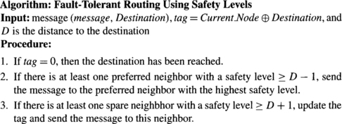
A faulty node has a safety level of 0. A safe node has a safety level of n (the diameter of the network). All nonfaulty nodes are initialized to a safety level of n. The levels of the other nodes are determined by the locations of faulty nodes. Intuitively, for a node to have a safety level of k, no more than (n – k − 1) neighbors can have a safety level of less than (k − 1). This will guarantee that for any incoming message destined to traverse k additional links, at least one neighbor along a preferred dimension will have a safety level of at least k − 1. It has been shown that this property enables the computation of safety levels of all nodes in (n − 1) steps by a local algorithm that in each step updates the safety level of a node as a function of the safety level of its neighbors from the previous step.
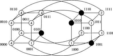
Consider a binary hypercube with four faulty nodes as shown in Figure 6.12 [351]. The nodes are labeled with their corresponding safety levels. Node 1100 has a safety level of 2. Thus every node at a distance of two hops from node 1100 can be reached by a path of length no more than 2. For example, consider a path to node 0110. If dimensions are traversed in increasing order, the dimension-order path is blocked by the faulty node 1010. However, an alternative path is available: via node 0100. Note that node 0100 adjacent to node 1100 is on the shortest path to node 0110 and has a safety level of 4. This example illustrates the global nature of the safety-level attribute. The exact distribution of the faults is unknown. However, the availability of shortest paths to nodes is encoded in the safety level, and this can be used to make local decisions about routing.
6.4.3 Routing Algorithms Based on Graph Search
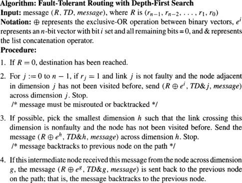
Often it is not possible to guarantee that the number of faults will be less than ![]() or the node degree. In this case, more flexible mechanisms are necessary to ensure that messages can be delivered if a physical path exists between two nodes. Routing algorithms based on graph search techniques provide the maximum flexibility. Message packets can be routed to traverse a set of links corresponding to a systematic search of all possible paths between a pair of nodes. Although the routing overhead is significant, the probability of message delivery in faulty networks is maximized. There have been several schemes for such search-based routing algorithms (e.g., [52, 62]). In the following we describe a fault-tolerant packet routing algorithm based on a depth-first traversal of binary hypercubes [52]. While specific computations may differ, the paradigm is certainly applicable to other point-to-point networks employing SAF or VCT switching mechanisms.
or the node degree. In this case, more flexible mechanisms are necessary to ensure that messages can be delivered if a physical path exists between two nodes. Routing algorithms based on graph search techniques provide the maximum flexibility. Message packets can be routed to traverse a set of links corresponding to a systematic search of all possible paths between a pair of nodes. Although the routing overhead is significant, the probability of message delivery in faulty networks is maximized. There have been several schemes for such search-based routing algorithms (e.g., [52, 62]). In the following we describe a fault-tolerant packet routing algorithm based on a depth-first traversal of binary hypercubes [52]. While specific computations may differ, the paradigm is certainly applicable to other point-to-point networks employing SAF or VCT switching mechanisms.
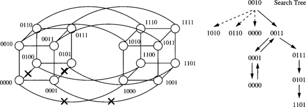
A major issue with exhaustive traversals of graphs or networks is that of visiting a node more than once. In the context of routing message packets in multipath networks, visiting a node more than once results in unnecessary overhead. Most approaches utilize state information maintained in the message header to avoid redundant visits. Consider a message structured as (R, TD, message) [52]. R is an n-bit vector that serves as the routing tag. If bit i in R is set, the message must traverse dimension i. When R = 0, the message has arrived at its destination. TD is the set of dimensions that the message has traversed. It is initialized to 0 at the source. As the message progresses through intermediate nodes, R and TD are updated. Routing at an intermediate node proceeds in three steps. First, the message is transmitted along a link on the shortest path to the destination. If all such paths are blocked by faulty components, the message must be misrouted to a neighboring node. However, we wish to avoid visiting any node more than once. This is realized as follows. In general, given an initial node, and a sequence of dimensions, c1, c2, …, ck, we can determine all of the nodes on the path from the source that are visited by traversing these dimensions. For example, starting from node 0110, a message traversing the dimensions 0, 2, and 3 will visit nodes 0111, 0011, and 1011, respectively. When a message is blocked by faults at an intermediate node, the list of dimensions traversed by the message up to this point can be used to compute the addresses of all of the nodes that have been visited by this message. Any adjacent nodes that belong in this set of nodes are no longer candidates for receiving the misrouted message. If all adjacent nodes have been visited or remain blocked by faults, the message backtracks to the previous node. Figure 6.13 shows an example of a search tree (i.e., sequence of nodes) generated by a message transmitted from node 0010 to node 1101. An algorithmic description of a routing algorithm based on depth-first search is provided in Figure 6.14. Optimizations to improve the efficiency of this implementation can be found in [52]. As in related approaches, each misrouting step lengthens the path between source and destination by two hops.
Related algorithms that are also based on depth-first search, but differing in some of the optimizations, can be found in [26, 28]. In particular, [28] describes an algorithm based on concurrent consideration of diagnosis and routing. The routing algorithm can proceed concurrently with on-line diagnosis of faulty nodes and links. The diagnosis algorithm is based on k-reachability and propagates fault information within a k-neighborhood. The approach is to devise a routing algorithm that can make use of concurrently available, and evolving, diagnostic information. As a result the initial message is injected into the network with a specification of the complete path from source to destination stored in the header. If no faults are encountered, the message is successfully routed to the destination along this path. At some intermediate node it may become evident that a node or link along this path has become faulty. This information may have just become available after the message has left the source. The intermediate node attempts to produce a new feasible path to the destination based on this updated diagnostic information. If such a path is not available and the message cannot be forwarded, the message is returned to the previous node on the path (i.e., a backtracking operation takes place). The routing algorithm is again invoked at this node. If the message is backtracked to the source, then it cannot be delivered. The result is an approach that produces a cooperative relationship between on-line k-reachability diagnosis and fault-tolerant routing.
The hyperswitch [62] is an adaptively routed network that supports circuit and packet switching and a set of backtracking routing algorithms for searching the network for uncongested and fault-free paths. The routing algorithm implemented by the hyperswitch is a best-first search heuristic. The routing probes for circuit-switched messages and the headers for packet-switched messages can be subjected to the same routing algorithm. Rather than an exhaustive depth-first search of the binary hypercube, the header maintains a channel history tag. The tag has n bits and records dimensions across which a header has backtracked. It can also be regarded as a record at a node of the dimensions across which a header has unsuccessfully tried to find a path. When a backtracking header is received and forwarded across another dimension at an intermediate node, the channel history tag is forwarded along with the message. The setting of the dimensions in this tag prevents the message from making traversals along certain dimensions and therefore revisiting portions of the network that may already have been searched. Effectively, portions of the search tree shown in Figure 6.13 are pruned. In Example 6.4, when the header backtracks to node 0011, the channel history tag might be set to 0010 and forwarded along with the message to node 0111. This will prevent the message from traversing dimension 1 at node 0111, and the header will be routed to node 1111 and then onto node 1101. The hyperswitch routing algorithm is programmable and can alternatively implement an exhaustive search or a hybrid search. In a hybrid search, the routing algorithm performs an exhaustive search when the message is within a specified distance from the destination. The hybrid approach is used to prevent excessive (and unnecessary) backtracking in large networks when the message is far from the destination. The trade-off is between the probability of finding a path versus finding a longer path via backtracking.
6.4.4 Deadlock and Livelock Freedom Issues
In the description of the preceding SAF techniques, deadlock freedom was not discussed. With the exception of [198], the original descriptions did not directly address deadlock freedom. For SAF networks in general, there are standard techniques for resolving the issue of deadlock freedom, some of which were described in Chapter 3. The preceding routing algorithms could adopt the following approach. The message buffers within each router are partitioned into B classes. These classes are placed in a strict order (a partial order actually will suffice). For example, if the number of buffer classes is the same as the maximum path length of any message, then as messages are routed between nodes, they are constrained to occupy a buffer in a class equal to the distance traversed to that point. With a known maximum distance and a corresponding number of buffers at each node, buffers are occupied in strictly increasing order and deadlock is prevented. The approach described in [198] produces maximum path lengths of (n + 1), and thus (n + 2) buffer classes would suffice. Typically, maximum path lengths, and therefore buffers at a node, depend upon the maximum number of faults. For routing algorithms based on graph search algorithms, the extent of the search would have to be controlled to bound the maximum path length, as a compromise between the probability of finding a path between any two nodes and the amount of buffer space required for deadlock freedom.
It is evident that fault-tolerant routing requires some form of misrouting to avoid faulty components. However, when messages are permitted to be routed farther away from the destination, the possibility of livelock must be addressed. The preceding techniques utilize deterministic approaches to prevent livelock by incorporating history information into the message header. A record of the history of the message is used in conjunction with knowledge of the structure of the network to bound the lifetime of a message packet in the network. The basic paradigm is one wherein the number of options for a message are guaranteed to be finite, and the routing algorithm ensures progress in exploring all of the options. A finite number of options can be created by using history information to ensure that nodes and links cannot be repeatedly visited by a message.
6.5 Fault-Tolerant Routing in Wormhole-Switched Networks
The use of small buffers in wormhole switching presents unique challenges in the design of fault-tolerant routing algorithms. Since blocked messages span multiple router nodes, the effects of faults are rapidly propagated through the routers and to other messages that compete for shared virtual channels. Since recovery from a fault is expensive in terms of time and resources, routing algorithms favor the incorporation of deadlock freedom by construction rather than recovery. The resulting algorithms are closely related to the permissible patterns of faulty components and the switching technique employed.
The most common approach is to route messages around fault regions, and to do so in a manner that avoids introducing new channel dependencies. The ability to successfully route messages around faulty regions depends on the shape of the fault region and the base routing algorithm that is used (i.e., adaptive or oblivious). Approaches typically involve adding resources such as virtual channels and enforcing routing restrictions among them. The following sections discuss fault-tolerant routing algorithms that have evolved for wormhole-switched networks to accommodate different fault regions.
6.5.1 Rectangular Fault Regions
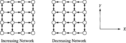
Consider the simplest fault model: block faults in a 2-D mesh network using the e-cube routing algorithm. Fault-free messages are routed in dimension order. When a block fault is encountered, the desired behavior of the routing algorithms is as shown in Figure 6.15. The e-cube path of the message from node S to node D passes through the block fault region, and one alternative (nonminimal) path for the message is as shown in the figure. However, traversal of this path would require messages to be routed from a column to a row (e.g., at point T in Figure 6.15). E-cube remains deadlock-free by preventing messages from traversing a row after traversing a column. Such traversals introduce new dependencies between channels in the vertical and horizontal direction, introduce cycles in the channel dependency graph, and therefore could lead to deadlocked message configurations. A solution to this problem for 2-D mesh networks proposed by Chien and Kim [58] is planar-adaptive routing, which was described in Section 4.3.1. This approach adds one additional virtual channel in the vertical direction. Now the set of virtual channels can be partitioned into two virtual networks as shown in Figure 6.16: the increasing network and the decreasing network. In the increasing (decreasing) network messages only travel in increasing (decreasing) X coordinates. The message shown in Figure 6.15 will be routed in the increasing virtual network. When the fault region is encountered, the message can be routed in the vertical direction to the top (or bottom) of the fault region. At this point the message may continue its progress in the horizontal direction.
Consider the example shown in Figure 6.15 where the message uses the increasing network. Assume the virtual channel 0 is used in the Y direction in the increasing network.
Since the fault regions are rectangular, messages only travel though intermediate nodes with nondecreasing values of the X coordinate. Further, if fault regions do not include boundary nodes, the ability to “turn the corner” around the fault region is guaranteed, and messages traverse any given column in only one direction; that is, there are no dependencies between the channels d1,0+ and d1,0– (see Section 4.3.1 for notation). Thus, there are no cyclic dependencies among the channels in the Y direction. Since channels in the X direction are strictly in increasing coordinates, there can be no cyclic channel dependencies involving both X and Y channels. A similar argument can be made for the decreasing network. Since messages only travel in one network or the other, routing is deadlock-free.
The preceding technique is very powerful and can be extended in several ways. Since the networks are acyclic, messages can be adaptively routed [58] along shortest paths: at an intermediate node, a message may be routed along either dimension. The only case where a message will be misrouted is when the destination node is in the same column or row, and the message is blocked by a fault region. As the preceding discussion demonstrated, routing remains deadlock-free. The technique can also be extended to multidimensional meshes using planar-adaptive routing. Recall from Section 4.3.1 that in planar-adaptive routing messages are adaptively routed in successive planes Ai formed by two dimensions, di and di+1. When fault regions are constrained to be block faults, any two-dimensional cross section of the fault region will form a rectangular fault region and will appear as shown in Figure 6.15.
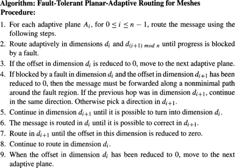
Note that when messages reduce the offset in dimension di to 0, they are routed in the next adaptive plane. As a consequence, messages cannot be blocked by a fault region in dimension di+1 after having reduced the offset in dimension di to zero. Therefore, messages are misrouted in only one dimension at a time. Since traffic in distinct adaptive planes that traverse the same physical link travel along separate virtual channels, and misrouting occurs only within one adaptive plane before messages are routed in the next adaptive plane, deadlock freedom is preserved. An algorithmic description of fault-tolerant planar-adaptive routing is provided in Figure 6.17.
The preceding techniques can be extended to tori as follows. Two virtual channels are required for each physical link to break the physical cycles created by the wraparound connections in the network. A solution for tori can be obtained simply by replacing each virtual channel in the mesh solution by two virtual channels. All of the arguments that characterize and demonstrate deadlock freedom for the mesh solution now apply to toroidal networks with appropriate routing restrictions over the wraparound channels to break the physical cycles. This solution requires six virtual channels for each physical channel.
The preceding techniques do encounter problems when fault regions occur adjacent to each other or include nodes on the boundary, as shown in Figure 6.18. When messages being misrouted around a fault region reach a boundary node such as R, the direction of the message has to be reversed. This introduces dependencies from channels di, j + to di, j – and vice versa, creating cyclic dependencies among the virtual channels in dimension j and cycles in the channel dependency graphs of the increasing and decreasing networks. The reason can be understood by observing that, logically, nodes on the boundary of a mesh are adjacent to a fault region of infinite extent. Messages cannot be routed around this fault region. The situation is equivalent to the occurrence of a concave fault region. Adjacent fault regions produce similar concavities as shown at node S. In the presence of concavities, paths in a 2-D mesh that are traversed by messages misrouted due to faults lose two important properties: (1) the X coordinate is no longer monotonically increasing or decreasing, and (2) new dependencies are introduced between channels in the vertical direction, producing cycles in the channel dependency graph. Ensuring that fault regions remain convex will require marking fault-free nodes as faulty. In this example, construction of a rectangular fault region will necessitate marking the first five rows of nodes in Figure 6.18 faulty. Similar examples can be constructed for the multidimensional case. This is clearly an undesirable solution and motivates solutions that make more efficient use of nonfaulty nodes.
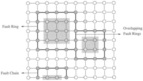
One such approach to reduce the number of functional nodes that must be marked as faulty was introduced by Chalasani and Boppana [49] and builds on the concept of fault rings to support more flexible routing around fault regions. Intuitively a fault ring is the sequence of links and nodes that are adjacent to and surround a fault region. Rectangular fault regions will produce rectangular fault rings. Figure 6.19 shows an example of two fault rings and a fault chain. If a fault region includes boundary nodes, the fault ring reduces to a fault chain. The key idea is to have messages that are blocked by a fault region misrouted along the fault rings and fault chains. For oblivious routing in 2-D meshes with nonoverlapping fault rings, and with no fault chains, two virtual channels suffice for deadlock-free routing around fault rings. These two channels form two virtual networks C0 and C1, each with acyclic channel dependencies, and messages travel in only one network (see Exercise 6.1).
However, this solution is inadequate in the presence of overlapping fault rings and fault chains. The reason is that the two virtual networks are no longer sufficient to remove cyclic dependencies between channels. Messages traveling in distinct fault rings share virtual channels as shown in Figure 6.19. As a result additional dependencies are introduced between the two virtual networks, leading to cycles. Furthermore, the occurrence of fault chains may cause messages that are initially routed toward the boundary nodes to be reversed. If we employed fault-tolerant planar-adaptive routing, such occurrences would introduce dependencies between the d1,0+ and d1,0– virtual channels in dimension 1, creating cyclic dependencies between them.
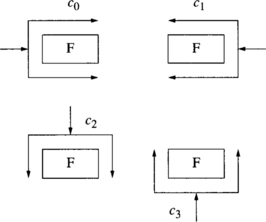
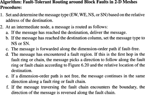
The solution proposed by Chalasani and Boppana [49] is to provide additional virtual channels to create disjoint acyclic virtual networks. The effect is to separate the traffic of the two fault rings that traverse the shared links. This can be achieved by providing two additional virtual channels per link, for a total of four virtual channels over each physical channel. Label these virtual channels c0, c1, c2, and c3. We may construct four virtual networks, each comprised of virtual channels of each type. Messages are assigned types based on the relative positions of the source and destinations and dimension-order routing. In a 2-D mesh, messages are typed as east-west (EW), west-east (WE), north-south (NS), or south-north (SN) based on the relative values of offsets in the first dimension. Routing is in dimension order until a message encounters a fault region. Depending on the type, the message is routed around the fault region as shown in Figure 6.20. The direction around the fault region is selected based on the relative position of the destination node. The WE messages use the c0 channels, with the remaining messages using the other channels as shown. The EW and WE messages may become NS and SN messages. However, the converse is not true. Thus, dependencies between channel classes are acyclic. Since fault regions are rectangular, dependencies within a fault region are also acyclic—the arguments are similar to those provided for fault-tolerant planar-adaptive routing. A brief description of the routing algorithm is presented in Figure 6.21.
The extension to fully adaptive routing can be performed in a straightforward manner. Assume the existence of any base, fully adaptive routing algorithm and the associated set of virtual channels. The only instance in which the progress of an adaptively routed message is impeded is when the message need only be routed in the last dimension, and progress in this dimension is blocked by a fault region. In this case, with four additional virtual channels, the preceding solution for oblivious routing can be applied. There is no real loss in adaptivity since the message has only one dimension that remains to be traversed. This approach effectively adds four virtual channels to support oblivious routing around fault regions, and transitions to this solution as a last resort. Once a message enters these virtual channels, it remains in these channels until it is delivered to the destination.
Figure 6.22 shows an example of routing around regions with overlapping fault rings. Two messages A and B have destinations and sources as shown. The former is an EW message, and the latter is a WE message. Message B is routed as a WE message around the fault region until it reaches the destination column where the type is changed to that of an NS message. The figure also illustrates the path taken by message A. Note that these two messages share a physical link where the fault rings overlap. Consider the shared link where both messages traverse the link in the same direction. If virtual channels were not used to separate the messages in each fault ring, one of the messages could block the other. An EW message can block a WE message and vice versa, resulting in cyclic dependencies. The separation of the messages into four classes, the use of four distinct virtual networks, and acyclic dependencies between these networks prevents the occurrence of deadlock.
If fault rings do not overlap, the above approach is easily extended to fully adaptive routing in tori with the following simple modification. Let us assume there exists a base set of virtual channels that provides fully adaptive deadlock-free routing in 2-D meshes. From the preceding discussion, four additional virtual channels are provided for routing around the fault rings [50], creating the four virtual networks. From Figure 6.20 it is apparent that the channel dependency graph of virtual channels within each of the virtual networks is acyclic. The presence of wraparound channels in the torus destroys this property. The cyclic dependencies introduced in the torus can be eliminated through the use of routing restrictions. Messages traveling in a virtual network are further distinguished by whether or not they will traverse the wraparound channel. These messages are routed in opposite directions around the fault region: messages that will (not) travel along the wraparound channel are routed in the counterclockwise (clockwise) direction around the fault region. Thus, the channel resources used by the message types are disjoint, and cyclic dependencies are prevented from occurring between them. The routing algorithm is essentially the same as the extension to fully adaptive routing in 2-D meshes, modified to pick the correct orientation around the fault ring when a message is blocked by a fault.
However, if fault rings in tori overlap, then messages that use the wraparound links share virtual channels with messages that do not use the wraparound links. This sharing occurs over the physical channels corresponding to the overlapping region of the fault rings. The virtual networks are no longer independent, and cyclic dependencies can be created between the virtual networks and, as a result, among messages. It follows from the preceding discussion that four more virtual channels [37] can be introduced across each physical link, creating four additional networks to further separate the message traffic over shared links. This is a rather expensive solution. The alternative is to have the network functioning as a mesh. In this case the benefits of a toroidal connection are lost.
A different labeling procedure is used in [43] to permit misrouting around rectangular fault regions in mesh networks. Initially fault regions are grown in a manner similar to the preceding schemes, and all nonfaulty nodes that are marked as faulty are labeled as deactivated. Nonfaulty nodes on the boundary of the fault region are now labeled as unsafe. Thus, all unsafe nodes are adjacent to at least one nonfaulty node. An example of faulty, unsafe, and deactivated nodes is shown in Figure 6.23. There are three virtual channels traversing each physical channel. These virtual channels are partitioned into classes. Nodes adjacent to only nonfaulty nodes have the virtual channels labeled as two class 1 channels and one class 2 channel. Nodes adjacent to any other node type have the channels partitioned into class 2, class 3, and class 4 channels. In nonfaulty regions of the network, a message may traverse a class 1 channel along any shortest path to the destination. If no class 1 channel is available, class 2 channels are traversed in two phases. The first phase permits dimension-order traversal of positive direction channels, and in the second phase negative direction class 2 channels can be traversed in any order (i.e., not in dimension order). The only time the fully adaptive variant of this algorithm must consider a fault region is when the last dimension to be traversed is blocked by a fault region necessitating nonminimal routing. Dimension (i + 1) and dimension i channels are used to route the message around the fault region. Messages first attempt routing along a path using class 3 channels and class 2 channels in the positive direction. Subsequently messages utilize class 4 channels and class 2 channels in the negative direction. Note that class 3 and class 4 channels only exist across physical channels in the vicinity of faults. The routing restrictions prevent the occurrence of cyclic dependencies between the channels, avoiding deadlock.

The paradigm adopted throughout the preceding examples has been to characterize messages by the direction of traversal in the network and therefore the direction and virtual channels occupied by these messages when misrouted around a fault ring. The addition of virtual channels for each message type ensures that these messages occupy disjoint virtual networks and therefore channel resources. Since the usage of resources within a network is orchestrated to be acyclic and transitions made by messages between networks remain acyclic, routing can be guaranteed to be deadlock-free. However, the addition of virtual channels affects the speed and complexity of the routers. Arbitration between virtual channels and the multiplexing of virtual channels across the physical channel can have a substantial impact on the flow control latency through the router [57]. This motivated investigations of solutions that did not rely on many (or any) virtual channels.
Origin-based fault-tolerant routing is a paradigm that enables fault-tolerant routing in mesh networks under a similar fault model, but without the addition of virtual channels [145]. The basic fault-free form of origin-based routing follows the paradigm of several adaptive routing algorithms proposed for binary hypercubes and the turn model proposed for more general direct network topologies. Each message progresses through two phases. In the first phase, the message is adaptively routed toward a special node. On reaching this node, the message is adaptively routed to the destination in the second phase. In previous applications of this paradigm to binary hypercubes, this special node could be the zenith node whose address is given by the logical OR of the source and destination addresses. Messages are first routed adaptively to their zenith and then adaptively toward the destination [184]. This phase ordering prevents the formation of cycles in the channel dependency graphs. Variants of this approach have also been proposed, including the relaxation of ordering restrictions on the phases [59]. In origin-based routing in mesh networks this special node is the node that is designated as the origin according to the mesh coordinates. While the approach is directly extensible to multidimensional networks, the following description deals with 2-D meshes.
All of the physical channels are partitioned into two disjoint networks. The IN network consists of all of the unidirectional channels that are directed toward the origin, while the OUT network consists of all of the unidirectional channels directed away from the origin. The orientation of a channel can be determined by the node at the receiving end of the channel. If this node is closer to the origin than the sending end of the channel, the channel is in the IN network. Otherwise it is in the OUT network. The outbox for a node in the mesh is the submesh comprised of all nodes on a shortest path to the origin. An example of an outbox for a destination node D is shown in Figure 6.24. Messages are routed in two phases. In the first phase messages are routed adaptively toward the destination/origin, over any shortest path using channels in the IN network. When the header flit arrives at any node in the outbox for the destination, the message is now routed adaptively toward the destination using only channels in the OUT network. As shown in the example in Figure 6.24, the resulting complete path may not be a minimal path. The choice of minimal paths is easily enforced by restricting messages traversing the IN network to use channels that take the message closer to the destination. The result of enforcing such a restriction on the same (source, destination) pair is also shown in Figure 6.24. The choice of the origin node is important. Since all messages are first routed toward the origin, hot spots can develop around the origin. Congestion around the origin is minimized when it is placed at one of the corners of the mesh. In this case, origin-based routing is equivalent to the negative-first algorithm derived from the turn model. We know from Chapter 4 that such routing algorithms are only partially adaptive. Placing the origin at the center improves adaptivity, but increases hot spot contention in the vicinity.
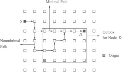
The fault-tolerant implementation of origin-based routing requires the fault regions to be square. Square regions are formed by starting from the rectangular fault regions created by preceding techniques and disabling additional nodes to ensure that the fault regions are square. A final step in setting up the mesh is for each nonfaulty node to compute and store the distance to the nearest fault region in the north, south, east, and west directions. The time required to compute this information and form the square fault regions depends on the network size, thus being bounded by the diameter of the mesh. Finally an origin node is selected such that the row and column containing the origin has no faulty nodes. If this is not possible, these techniques can be applied to the largest fault-free submesh, disabling all remaining nodes. Central to this routing algorithm is the identification of a set of nodes in the diagonal band of the destination. The diagonal band of a node s is the set of all nodes in the outbox of s that lie on a tridiagonal band toward the origin. The X andY offsets from node s to any node in the diagonal band differ by at most 1. An example of a diagonal band is shown in Figure 6.25. The useful property of nodes in the diagonal band is that there exists a fault-free path from any one of these nodes to the destination node using channels in the OUT network [145]. Such nodes are referred to as safe nodes. The property of safety of nodes in the diagonal band is ensured by square fault regions. If fault regions are square, then any message at a safe node that is blocked by a fault region is guaranteed the existence of a path around the fault region, through nodes within the outbox, and reaching a destination node on the other side of the fault region. Square fault regions guarantee the safety of nodes in the diagonal band.
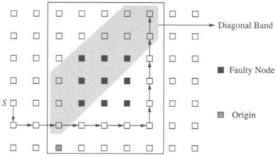
Fault-tolerant routing proceeds as follows. A message is routed adaptively as before in the IN network toward the origin until it arrives at a node in the outbox of the destination or the origin (by definition the origin is in the outbox of the destination). Since the origin is in a fault-free column/row and fault regions are square, a free output channel in the IN network is guaranteed to exist during this phase. Once the message arrives at a node in the outbox of the destination, if the message is at a safe node, then a path is guaranteed to be available to the destination using only channels in OUT. If the message is not at a safe node, routing continues in the IN network. At an intermediate node the distance to the nearest safe node in each direction can be computed. This is compared to the distance of the nearest fault in that direction. If the safe node is closer than fault regions, the message is routed to that node using only channels in IN or OUT. By virtue of their construction, safe nodes guarantee the availability of paths by routing around fault regions. If the message encounters a fault region, it can be routed around the fault region until it can be routed back up to the diagonal band. This case is illustrated in Figure 6.25.
Routing occurs in three phases with three successive goals: (1) route to the outbox, (2) route to a safe node in the outbox, and (3) route to the destination. This technique can be applied to meshes in the absence of virtual channels. Other optimizations such as increasing the size of the safe region in the outbox and trading adaptivity for simplicity and speed are described in [145]. A functional description of the algorithm is shown in Figure 6.26.
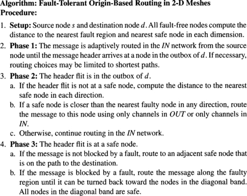
Rectangular and square fault regions provide some form of nondecreasing property in coordinates of misrouted messages. This property is exploited to prevent the occurrence of deadlocked message configurations. However, the construction of rectangular fault regions by the marking of fault-free routers and links as faulty can lead to significant underutilization of resources. While permitting arbitrary fault patterns is still an elusive goal, it would be desirable to relax the restrictions on the shape of the fault regions.
To help achieve this goal, the concept of fault rings can be extended in a minimal manner to account for certain classes of nonconvex fault regions [50]. Consider the class of fault regions in n-dimensional mesh networks where any 2-D cross section of the fault region produces a single rectangular fault region. Such a fault model is referred to as a solid fault model [50]. Figure 6.27 provides an example of a nonconvex fault region that follows the solid fault model, and a message being routed along a fault ring around the fault region. As in previous techniques, for nonoverlapping fault rings and nonfaulty boundary nodes, message types are distinguished by the relative position of the destination when the message is generated. For deterministic routing, we initially have EW and WE messages. When the message eventually arrives at the destination column, the message type is changed to NS or SN depending on the relative location of the destination. When a message encounters a fault, the rules for routing the message along the fault ring are shown in Table 6.2. There are four virtual channels over each physical channel: c0, c1, c2, and c3. As in preceding techniques, each set of channels implements a distinct virtual network.
Table 6.2
Routing rules for solid fault regions.
| Message Type | Position of Destination | F-Ring Orientation |
| WE | Row above current row | Clockwise |
| WE | Row below current row | Counterclockwise |
| EW | Row above current row | Counterclockwise |
| EW | Row below current row | Clockwise |
| NS or SN | Either position | Either orientation |
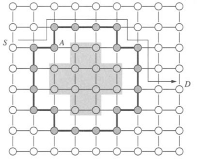
If a message must travel along a fault ring before encountering a fault region (i.e., as shown in Figure 6.27 at node A), then the message must continue to be routed in the same direction along the fault ring. Otherwise the message follows the direction stated in Table 6.2. Each message type is routed in a distinct virtual network. From the routing rules we can observe that the channel dependency graph within a virtual network is acyclic.
Further, messages can only transition from WE or EW channels to NS or SN channels but not vice versa. Thus, the relation between these virtual networks remains acyclic, and therefore routing remains deadlock-free. Note that these rules apply to rings that do not overlap and that do not include nodes on the boundary of the mesh.
6.5.2 Software-Based Fault-Tolerant Routing
The addition of virtual channels and enforcement of routing restrictions between them impacts the design and implementation of the routers. However, in environments where the fault rates are relatively low, the use of expensive, custom, fault-tolerant routers often cannot be justified. Moreover, contemporary routers are compact, oblivious, and fast. Ideally, we wish to retain these features and minimize both the additional hardware support required in the routers and the impact on the router performance. It would also be advantageous to employ techniques that would not require expensive modifications to the routing control to implement rerouting restrictions. The development of these techniques is governed by the relationship between the MTBF and the MTTR. When MTTR ![]() MTBF, the number of faulty components in a repair interval is small. In fact, the probability of the second or the third fault occurring before the first fault is repaired is very low. In such environments, software-based rerouting can be a cost-effective and viable alternative [333].
MTBF, the number of faulty components in a repair interval is small. In fact, the probability of the second or the third fault occurring before the first fault is repaired is very low. In such environments, software-based rerouting can be a cost-effective and viable alternative [333].
The software-based approach is based on the observation that the majority of messages do not encounter faults and should be minimally impacted, while the relatively few messages that do encounter faults may experience substantially increased latency, although the network throughput may not be significantly affected. The basic idea is simple. When a message encounters a faulty link, it is removed from the network or absorbed by the local router and delivered to the messaging layer of the local node’s operating system. The message-passing software either (1) modifies the header so that the message may follow an alternative path or (2) computes an intermediate node address. In either case, the message is reinjected into the network. In the case that the message is transmitted to an intermediate node, it will be forwarded upon receipt to the final destination. A message may encounter multiple faults and pass through multiple intermediate nodes. The issues are distinct from adaptive packet routing in networks using packet switching or VCT switching. Since messages are routed using wormhole switching, rerouting algorithms and the selection of intermediate nodes must consider dependencies across multiple routers caused by small buffers (< message size) and pipelined data flow. Since messages are reinjected into the network, dependencies are introduced between delivery channels at a router and the injection channels. These dependencies are introduced via local storage for absorbed packets. Memory allocation must ensure that sufficient buffer space can be allocated within the nodes or interfaces to avoid creating deadlock due to the introduction of these dependencies.
Since messages are removed from the network and reinjected, the problems of routing in the presence of concave fault regions are simplified. Consider the case of messages being routed obliviously using e-cube routing in a 2-D torus. Figure 6.28 illustrates an example of software-based rerouting in the presence of concave fault regions. The resulting routing algorithm has been referred to as e-sft [333]. In step 1 a message from the source is routed through an e-cube path to the destination and encounters the fault region at node A. The message is absorbed at the node, and the header is modified by the messaging layer to reflect the reverse path in the same dimension, using the wraparound channels. The message again encounters the fault region at node B and is routed to an intermediate node in the vertical direction in an attempt to find a path around the fault region. This procedure is repeated at intermediate nodes E and F before the message is successfully routed along the wraparound channels in the vertical dimension to the destination node D. While the path and the sequence of routing decisions to find the path in the preceding example are easy to convey intuitively, the messaging layer must implement routing algorithms that can implement this decision process in a fully distributed manner with only local information about faults. These rerouting decisions must avoid deadlock and livelock. This is realized through the use of routing tables and by incorporating additional information in the routing header to capture the history of encounters with fault regions by this message. The important characteristic of this approach is that messages are still routed in dimension order between any pair of intermediate nodes.
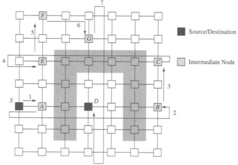
Figure 6.28 An example of software-based fault-tolerant routing (e-sft) in the presence of concave fault regions.
In order to keep track of the manner in which a message is rerouted, the header contains a 2-bit flag called the direction flag (DF). The DF is used to record the history of encounters with fault regions. For example, the message from S to D in Figure 6.28 will initially have a DF value of (00). When a fault region is encountered, DF is changed to (01), prior to routing in the reverse direction along the wraparound channel. Since fault-free routing is dimension order, a DF value of (10) would imply the message had attempted to traverse the X dimension in both directions and is now trying to traverse the Y dimension. The exception to this interpretation occurs when the source and destination nodes are in the same column. In this case the message will attempt the Y dimension first, and the interpretation of DF is reversed; that is, (00) and (01) ((10) and (11)) refer to the Y dimension (X dimension). A rerouted message may also encounter faults. The DF value in the header is only modified when the message is absorbed at a node. It enables e-sft routing to keep track of the directions along each dimension that have been attempted and therefore aid in rerouting decisions. There are three additional fields that are required in the header. A faulted status bit (F) indicates that the message has encountered at least one fault and is being rerouted. This bit enables a node to distinguish between messages destined for the local node and messages that must be forwarded. A prevent flag (PF) status bit is used to prevent the occurrence of certain livelock situations by recording a traversal through all DF values. A 2-bit reroute table field (RT) specifies one of three routing tables to be used for rerouting decisions. Finally, since messages may be routed through intermediate nodes, there must be two sets of address fields. The first records the final destination address (X-Final, Y-Final). This is an absolute address. The second is used for routing the messages and is an offset within each dimension (X-Dest, Y-Dest). The message header now appears as shown in Figure 6.29. Note that the routers only process the offset fields and set the F bit. All of the remaining header processing is done in software and only when messages encounter faults. Thus, router operations are minimally impacted.
![]()
Figure 6.29 Header format for software-based routing. (DF = direction flag; F = faulted status bit; PF = prevent flag; RT = reroute table; X-Dest = X coordinate offset; X-Final = X coordinate of the destination; Y-Dest = Y coordinate offset; Y-Final = Y coordinate of the destination.)
Let the coordinates of the destination node be (xd, yd) and the current node be (xc, yc). The offsets to the destination at any intermediate node can be computed as Δx and Δy in each dimension. The network hardware routes messages using traditional dimension-order routing based on the X-Dest and Y-Dest fields in the message header. If the outgoing channel at a router is faulty, the router sets the F bit and routes the message to the local processor interface. This causes the message to be marked as a faulted message and ejected to the local messaging layer. If the F bit is set, the messaging software checks the X-Final and Y-Final fields to determine if the message is to be delivered locally. If the message is not to be delivered locally, a rerouting function is invoked. The X-Dest and Y-Dest fields are updated, and if necessary the DF, PF, and RT flags are modified. The initial rerouting function depends on the relative address of the first node where a fault is encountered and the final destination. Tables 6.3–6.5 describe the rerouting rules. The notation ![]() refers to the coordinates of the next node in the path using the short (i.e., s) path along the y dimension. The notation l refers to the choice of the longer path. The rerouting algorithm implemented in the messaging layer is described in Figure 6.30.
refers to the coordinates of the next node in the path using the short (i.e., s) path along the y dimension. The notation l refers to the choice of the longer path. The rerouting algorithm implemented in the messaging layer is described in Figure 6.30.
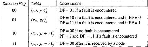
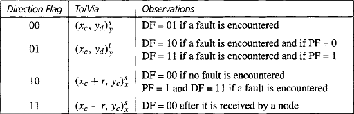
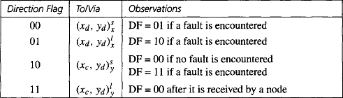
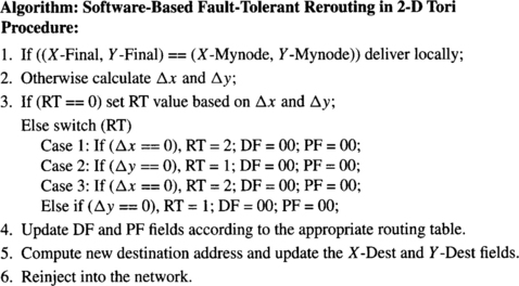
6.5.3 Unconstrained Fault Regions
Many of the early approaches to fault-tolerant routing did not adopt the approach of placing constraints on the shape of the fault regions. Rather, these techniques focused on rerouting around single faulty nodes and links. Since complete knowledge of the patterns of occurrences of faults is not assumed, these techniques are not generally applicable to cases where larger fault regions must be supported. In these instances, the routing algorithms discussed here must rely on fault recovery techniques to prevent deadlock. Consequently, guarantees of message delivery are made under conditions very different from those of the preceding techniques. However, these techniques have minimal impact on the design of the routers enabling them to remain compact and fast. Thus, they are attractive in environments with low fault rates.
The turn model described in Chapter 4 can be modified to handle the occurrence of faulty components. The example described here is the nonminimal version of the negative-first routing algorithm for 2-D meshes. Recall that this algorithm operates in two phases: the message is routed in the negative direction in each of the dimensions in the first phase, and then messages are routed in the positive directions in the second phase. The fault-tolerant nonminimal version routes adaptively in the negative direction, even farther west or south than the destination. For example, this is the path taken by message A in Figure 6.31. During this phase the message is routed adaptively and around faulty nodes or links. The exception occurs when a message being routed along the edge of the mesh in the negative direction encounters a faulty node. In the second phase, the message is routed adaptively in the positive directions to the destination, unless it reaches the destination column, in which case there is only one path to the destination. However, by permitting the message to be routed further west and south than the destination, more paths to the destination are created for the second phase, increasing the possibility that messages can be routed around a single faulty component. Modifications to the routing logic of the base negative-first algorithm are simply intended to increase the possibility of finding an alternative path when blocked by a faulty component, particularly along an edge of the mesh. The behavior that is permitted in this case is shown by message B in Figure 6.31. Such a single misroute to avoid a faulty component does avoid deadlock. The number of faults that can be tolerated is one less than the number of dimensions. This has been generalized to avoid up to (n − 1) faults in n-dimensional meshes [131]. The version of this algorithm for 2-D meshes is provided in Figure 6.32.
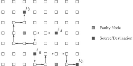
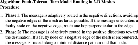
The advantage of this approach is that no virtual channels are required. From a practical point of view, in environments where MTTR ![]() MTBF, it is likely that no more than a single fault will occur within any repair interval. In this case the turn model approach can provide gracefully degraded communication performance in 2-D meshes until the faulty component can be replaced. Meanwhile the hardware architectures of the routers have been minimally impacted and remain compact and fast. For higher-fault-rate environments, more robust techniques that can provide delivery guarantees are desirable.
MTBF, it is likely that no more than a single fault will occur within any repair interval. In this case the turn model approach can provide gracefully degraded communication performance in 2-D meshes until the faulty component can be replaced. Meanwhile the hardware architectures of the routers have been minimally impacted and remain compact and fast. For higher-fault-rate environments, more robust techniques that can provide delivery guarantees are desirable.
The dimension reversal (DR) approach defined by Dally and Aoki [73] produces gracefully degradable network performance in the presence of faults by dividing messages into classes. Each message is permitted to be routed in any direction. However, if a message is routed from a channel in dimension di to a channel in dimension dj < di, a DR counter maintained in the message header is incremented. This DR counter is used to prevent the occurrence of cycles in the channel dependency graph. A static approach to doing so in multidimensional meshes creates r virtual networks by using r virtual channels across each physical channel. All messages are initialized with their DR values equal to zero. Messages are injected into virtual network 0 and permitted to be routed in any direction toward the destination. Misrouting is also permitted, although it should be controlled to ensure livelock freedom. When a dimension reversal takes place, the message moves into the next virtual network. Messages that experience greater than (r − 1) dimension reversals are routed in dimension order (i.e., deterministic, nonadaptive routing) in the last virtual network. This approach can require a large number of virtual channels.
An alternative dynamic version of this approach has only two virtual networks: the adaptive network and the deterministic network. Messages are now injected into the adaptive network. These messages can be routed in any direction using only adaptive channels and with no constraints on the number of misroutes other than those required to ensure livelock freedom. However, if a message must block waiting for a free channel at any node, the message may only block on channels being used by messages with a higher value of the DR counter. If virtual channels are labeled with the DR value of the message currently using the channel, this is easy to check. If all outgoing channels are being used by messages with lower DR values, the message enters the deterministic network, where it remains while following a fixed dimension-order path to the destination. The ordering of messages in the adaptive network prevents cycles of messages waiting on themselves. Messages only transition into the deterministic network and never the other way around. Therefore, deadlock freedom is guaranteed in the fault-free case. Previous approaches have placed strict ordering requirements on resource usage (i.e., channels) to prevent cyclic dependencies. This approach is a bit different in that the message population is partitioned into groups by virtue of the values of their DR counters. Waiting is based on the DR values of the messages rather than channels or dimensions, and messages are prevented from waiting on themselves.
The simulation results provided in [73] show graceful degradation in average message latency and network throughput with relatively high fault rates. However, in the presence of faults, deadlock may still occur. If a physical channel fails, all messages that are constrained to use the deterministic network and cross that physical channel will be blocked indefinitely. These messages cannot be delivered and can eventually lead to deadlocked configurations of messages, although the routing freedom otherwise provided by the DR scheme makes this highly unlikely. To guarantee deadlock freedom in the presence of faults, some form of fault recovery mechanism will be necessary.
A closer look at existing wormhole-switched routing algorithms can lead to several approaches to making these routing algorithms resilient to faults, although guaranteeing deadlock freedom is more difficult to achieve. Consider a minimal fully adaptive routing algorithm such as DP [91]. A simple extension permits an unprofitable adaptive channel to be used if no deterministic channel has been used by the message up to that point. This will permit the message to route around faulty regions with maximum flexibility before making use of a deterministic channel. However, even if the message has traversed a deterministic channel, misrouting can still be permitted in dimensions lower than that of the last deterministic channel traversed. This will prevent cyclic dependencies from forming among deterministic channels, and thus the extended channel dependency graph remains acyclic. However, from the point of view of guaranteeing deadlock freedom, situations may still arise where a message may have to block on a (deterministic) channel. If this channel is faulty, deadlock may result. In this case we would recommend coupling deadlock recovery schemes outlined in Section 6.7 with these schemes. This approach becomes more viable as the MTTR becomes increasingly smaller relative to the MTBF of the network components.
However, routing algorithms can be made more resilient to faults by combining routing techniques that support fully adaptive nonminimal routing. For example, it is possible to combine the theory of deadlock avoidance proposed in Section 3.1.3 with the turn model described in Section 4.3.2. This approach was followed in the fault-tolerant routing algorithm proposed in [93, 95] for n-dimensional meshes using wormhole switching. Each physical channel is split into four virtual channels. Virtual channels are grouped into four sets or virtual networks. The first virtual network consists of one virtual channel in each direction. It is used to send packets toward the east (X-positive). It will be referred to as the eastward virtual network. The second virtual network also consists of one virtual channel in each direction. It is used to send packets toward the west (X-negative), and it will be referred to as the westward virtual network. When the X coordinates of the source and destination nodes are equal, packets can be introduced in either virtual network. The routing algorithms for eastward and westward virtual networks are based on nonminimal west-last and east-last, respectively. Once a packet has used a west (east) channel in the eastward (westward) virtual network, it cannot turn again. However, 180-degree turns are allowed in Y channels except in the east (west) edge of the mesh. This routing algorithm is fully adaptive nonminimal. It is deadlock-free, as shown in Exercise 3.3 for 2-D meshes. While routing in the eastward (westward) virtual network, it tolerates faults except when routing on the east (west) edge. In order to tolerate faults in the edges, two extra virtual networks are used. The extra eastward (westward) virtual network is used when a fault is met while routing on the west (east) edge of the mesh. The resulting routing algorithm is very resilient to faults under both the node failure and the link failure models [93, 95]. Figure 6.33 shows the paths followed when some channels fail. Figure 6.34 shows the paths followed when some nodes fail. This approach also supports rectangular fault regions.
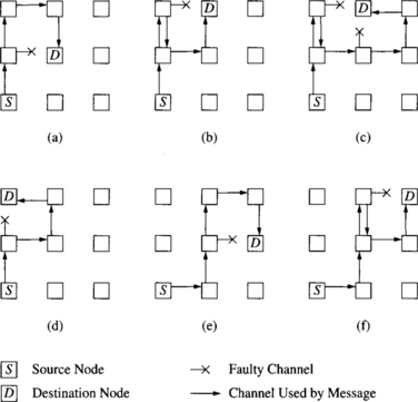
Figure 6.33 Routing examples with faulty channels on a 2-D mesh: (a) destination is not in any of the edges; (b) destination is in the upper edge and the message encounters one fault; (c) destination is in the upper edge and the message encounters two faults; (d) destination is in the upper-left corner; (e) destination is in the right edge; and (f) destination is in the upper-right corner.
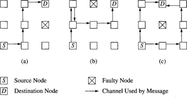
Figure 6.34 Routing examples with faulty nodes on a 2-D mesh: (a) destination is in the upper-right corner, and there is a faulty node in the right edge; (b) destination is in the upper-right corner, and there is a faulty node in the upper edge; and (c) destination is in the upper edge. Case (c) shows two alternative paths.
6.6 Fault-Tolerant Routing in PCS and Scouting Networks
The PCS switching mechanism described in Chapter 2 supports the flexible routing of the header to avoid faulty regions of the network. Potential paths from source to destination are searched by routing a header flit through the network along a path following a depth-first search of the network. The header acquires virtual links as it is routed adaptively toward the destination. When the header is blocked by a fault and none of the output channels along a path to the destination are available, it may be routed along nonminimal paths. If all candidate output channels at an intermediate router are busy, the header backtracks over the last acquired virtual link, releases the link, and the search is continued from the previous node. History information can be maintained at each individual router rather than within the header to ensure that a particular physical path out of a router will not be searched by the same message more than once. Within each router a 2n-bit mask, where n is the number of dimensions, is associated with each input virtual channel. This mask is initialized when the header first arrives at the router. When a header backtracks across a virtual channel and back to the router, the corresponding mask bit is set. Therefore, the routing function will prevent the header from being forwarded across this channel if it backtracks to this node in the future. All channel masks are stored locally. While this approach will prevent a header from traversing the same link twice, without additional support it will not prevent the header from visiting the same node twice. In general, limiting misroutes can be more effective in preventing multiple visits to the same node, while keeping the header size small.
After the header arrives at the destination and a virtual circuit has been successfully established, data are pipelined from the source to the destination. The attractive feature of this approach is the ability to combine the high performance that can be achieved with pipelined data flow with the conservative approach to finding fault-free paths through the network. The advantages of this approach over algorithms using wormhole switching are that performance is less sensitive to the shape of the fault regions and deadlock freedom is independent of the shape of the fault region.
One approach to the use of PCS for fault-tolerant routing is found in a family of misrouting backtracking algorithms. This family is referred to as MB-m [126] and is a set of backtracking algorithms with the routing restriction that less than or equal to m unprofitable links may be allowed in a path. With the history information distributed throughout the nodes, the header flit or probe consists of a vector of dimension offsets, a backtrack flag, and a misroute counter. Consider the following example of routing in a 2-D mesh as shown in Figure 6.35.
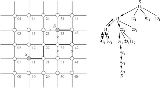
By permitting a larger number of misroutes, the algorithm can be made resilient to a larger number of faults. This family of algorithms is referred to as the misrouting backtracking with m misroutes (MB-m) class of algorithms. Deadlock freedom follows from the fact that the header does not block holding resources. Livelock freedom is guaranteed by limiting the number of misroutes. By keeping track of the outgoing links that have been searched at a node by a backtracking header, livelock is avoided, although the header may eventually backtrack to the source when the network is congested. At this point some higher-level algorithm must be available to prevent unlimited retries. A description of the MB-m algorithm is shown in Figure 6.36.
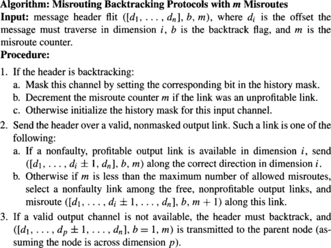
The MB-m algorithms are very conservative in the sense that data flits are not injected into the network unless the path has been set up. The result is very robust algorithms for large numbers of faults. This is particularly desirable in systems that experience large periods of unattended operation or high fault rates (e.g., space-borne embedded systems). However, when message sizes are small and fault rates relatively low, the overhead of an a priori path setup can be substantial. In such environments, an attractive option is to be able to dynamically configure the flow control protocols employed by the routers. Routing algorithms can be designed such that in the vicinity of faulty components messages use PCS-style flow control, where controlled misrouting and backtracking can be used to avoid faults and deadlocked configurations. At the same time messages use wormhole-switching flow control in fault-free portions of the network with the attendant performance advantages. Messages are routed in two phases—a fault-free phase and a faulty phase. Messages may transition between these two phases several times in the course of being routed between a source and destination node. Routing algorithms designed based on such flow control mechanisms are referred to as multiphase routing algorithms [79]. Such dynamically configurable flow control protocols can be configured using variants of scouting switching described in Chapter 2.
The following description presents a two-phase routing algorithm. Message routing proceeds in one of two phases: an optimistic phase for routing in fault-free network segments and a conservative phase for routing in faulty segments. An example of a two-phase (TP) algorithm is shown in Figure 6.37. The optimistic phase uses a fully adaptive, minimal, deadlock-free routing function based on DP (see Section 4.4.4). The conservative phase uses a form of MB-m. The switching technique is scouting switching with a scouting distance of K.
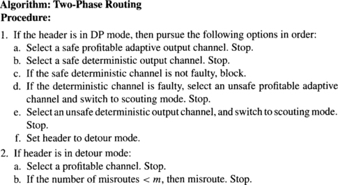
The virtual channels on each physical link are partitioned into restricted and unrestricted partitions. Fully adaptive minimal routing is permitted on the unrestricted partition (adaptive channels), while only deterministic routing is allowed on the restricted partition (deterministic channels). Channels are marked as safe or unsafe [198, 351] depending on the number of faulty links/nodes within the immediate neighborhood. The definition of the extent of this neighborhood for determining the safe/unsafe designation can be quite flexible. The purpose is simply to serve as a warning that traversal of this channel will move the message into the vicinity of faulty nodes and links. Each output virtual channel is provided with a counter to keep track of positive and negative acknowledgments from the headers. The channel also maintains the current value of the scouting distance, K, for comparison with the counter value. Initializing this output value to 0 is equivalent to using wormhole switching.
The selection function uses a priority scheme in selecting candidate output channels at a router node. First, the selection function examines the safe adaptive channels. If one of these channels is not available, either due to the channel being faulty or busy, the selection function examines the available safe deterministic channel. If the safe deterministic channel is busy, the routing header blocks and waits for that channel to become free. If a safe adaptive channel becomes free before a deterministic channel is freed, then the header is free to take the adaptive channel. If the deterministic channel is faulty, the selection function will return a profitable adaptive channel, regardless of whether it is safe or unsafe. The selection function will not select an unsafe channel over an available safe channel. An unsafe channel is selected only if it is the only alternative other than misrouting or backtracking. When an unsafe profitable channel is selected as an output channel, the message enters the vicinity of a faulty network region. This is indicated by setting a status bit in the routing header. Subsequently, the counter values of every output channel traversed by the header are initialized to K to implement scouting switching and permit header backtracking to avoid faults if the need arises. Flow control is now more conservative, supporting more flexible algorithms in routing around faulty regions. If no unsafe profitable channel is available, the header changes to detour mode and records this status in the header.
In detour mode, the normal positive acknowledgments generated by scouting switching are not transmitted. Therefore, data flits do not advance, and the header is free to be routed around the faulty region. During the construction of the detour, the routing header performs a depth-first, backtracking search of the network using a maximum of m misroutes. Only adaptive channels are used to construct a detour. The detour is complete when all the misroutes made during the construction of the detour have been corrected or when the destination node is reached. When the detour is completed, acknowledgments flow again and data flits resume progress. Note that all channels (or none) in a detour are accepted before the data flits resume progress. This is required to ensure deadlock freedom.
It is clearly desirable to have messages that do not encounter faults to be routed optimistically with wormhole switching. With respect to the conservative phase, several alternatives are possible. For example, an alternative implementation for the conservative phase is to avoid the usage of the safe/unsafe designation for the channels and to continue optimistic routing using wormhole switching until forward progress is stopped due to faults. At this point, a detour can be constructed using only the header and increased misrouting as necessary. When a detour is completed, one acknowledgment is sent to resume the flow of the data flits. Note that in this case we always have K = 0, and therefore no positive or negative acknowledgments are transmitted. Messages flow until either they are delivered or detours are the only option. In general, we expect that without the use of acknowledgments detours will have to be constructed more often. With the use of acknowledgments and a scouting distance, the header is permitted to backtrack a few links if necessary and potentially avoid costly detour construction. In general, this alternative for the conservative phase (i.e., detour construction only) is a trade-off between acknowledgment traffic bandwidth and the time spent in constructing detours.
Figure 6.38 shows an example of two-phase routing with seven node failures and m = 3. With unsafe channels and K initially set to 0, the routing header routes to node B, where it is forced to cross an unsafe channel. The value of K is increased to 3, and the header routes profitably to node A, with the data flits advancing until node B. At node A, the routing header cannot make progress toward the destination and therefore enters detour mode. The header is misrouted upward. After two additional misroutes the header can no longer be misrouted due to the limit on m. The routing header then is forced to backtrack to node A. Since there are no other output channels to select, the routing header is forced to backtrack to node C. From there, it is misrouted twice downward to where a profitable path to the destination can be found. In this example, the detour is completed when the destination is reached. Further, notice that data flits do not advance while the header is in detour mode. Thus, the first data flit is still at node B when the header is delivered to the destination.
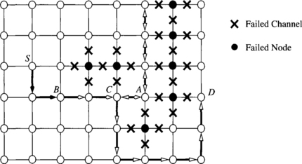
The distinguishing features of this approach are (1) it does not rely on additional virtual channels over that already needed for fully adaptive routing; (2) the performance is considerably better than conservative fault-tolerant routing algorithms with equivalent reliability; (3) it is based on a more flexible fault model (i.e., one that supports link and/or node faults and does not require convex fault regions); (4) it is compatible with existing techniques for recovery from dynamic or transient failures of links or switches (Section 6.7); and (5) it provides routing algorithms greater control over hardware message flow control, opening up new avenues for optimizing message-passing performance in the presence of faults. However, router complexity is increased although required architectural support does not appear to be on the critical path for router operation [79]. This approach does have a more complex channel model that can affect link speeds. For a low to moderate number of faults, configurable flow control mechanisms can lead to deadlock-free, fault-tolerant routing algorithms whose performance is superior to more conservative routing algorithms with comparable reliability. In a network with a large number of faults, the TP’s partially optimistic behavior results in severe performance degradation [79].
6.7 Dynamic Fault Recovery
Often component failures can occur during network operation, interrupting the transmission of messages across a link or router. We refer to such failures as dynamic failures. Dynamic failures may be permanent in nature. This is in contrast to transient failures, where component operation may be intermittent. For example, a channel may periodically drop a flit or corrupt the contents of the message. In either case, failures may interrupt a message in progress across a link or router. Pipelined communication mechanisms such as wormhole switching or PCS are particularly susceptible to such faults since messages are buffered across multiple routers and data flits do not contain routing information. Packet-switching mechanisms are amenable to link-level error detection and retransmission with a copy of the packet on either side of the link to prevent loss of data, and eliminate the need for buffering data at the source. With any of the pipelined switching mechanisms, messages are spread over multiple links and present some unique difficulties in recovering from dynamic faults. This section focuses on techniques for recovery from such occurrences.
6.7.1 Base Mechanisms
The ability to tolerate dynamic failures in message pipelines places additional requirements on the basic functionality of the network routers and interfaces. Consider the occurrence of a link failure as shown in Figure 6.39. The figure shows a message in transit between nodes SA and DA. The last flit of the message has left SA and is currently in node LA. The link marked in the network now fails. The portions of the message above the failed link continue to make progress toward the destination. The portions of the message below the failed link, starting with the flits in the output buffers of router RA, block in place. These data flits have no routing information associated with them. Therefore, they cannot be rerouted and block indefinitely holding resources, possibly leading to deadlock as shown in Figure 6.1.
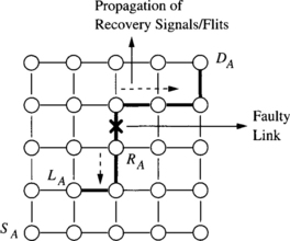
This situation places new requirements on the functionality of switching techniques and associated routing algorithms. There are at least two basic approaches to deal with such orphaned data flits. In one approach, header information is maintained through the routers that contain flits of the message. When messages are interrupted, a new message can be constructed with the stored header information, and the (relatively) smaller message can be forwarded along an alternative path to the destination. This will be referred to as flit-level recovery. Messages are injected only once into the network and recover from link-level dynamic and transient failures. Alternatively, the blocked data flits can be recovered and discarded from the network, the router buffers freed, and the message retransmitted from the source. In this case, the source and destination must synchronize message delivery or drop messages. This requires that the message be buffered at the source until it can be asserted that it has been delivered either explicitly through acknowledgments or implicitly through other mechanisms. This will be referred to as message-level recovery to denote the level at which recovery takes place. Implementations of each basic approach are described in the following.
6.7.2 Flit-Level Recovery
Reliable message delivery can be handled by end-to-end protocols that utilize acknowledgments and message retransmission to synchronize delivery of messages. Messages remain buffered at the source until it can be asserted that the message has been delivered. If we consider packet switching, more efficient alternatives exist for ensuring reliable end-to-end message delivery. Error detection and retransmission/rerouting can be implemented at the link level. A message must be successfully transmitted across a link before it is forwarded. With some a priori knowledge of the component failure rates, fault-tolerant routing algorithms can be developed where packets are injected into the network exactly once and guaranteed to be delivered to the destination by rerouting around faulty components. The difficulty in applying the same approach to wormhole-switched messages has been that the message packets cannot be completely buffered at each router and are spread across multiple routers when the header flit blocks. Thus, link-level monitoring and retransmission are difficult to realize on a message packet basis. The Reliable Router developed at the Massachussets Institute of Technology [74, 75] has implemented a novel approach utilizing a flit-level copying and forwarding algorithm to solve this problem and realize exactly-once injection and subsequent delivery of all packets in wormhole-switched networks.
Networks of reliable routers utilize three virtual networks. Five virtual channels are provided across each physical channel. Two of these virtual channels are used to implement an adaptive network where messages may utilize any outgoing channel from a router. Two more virtual channels are utilized to implement a dimension-ordered network where messages traverse links in dimension order. The two sets of dimension-order channels are used by packets at two priority levels. The two priorities are used with distinct resources to prevent software deadlocks. The remaining virtual channel is used as part of a network that implements the turn model for fault-tolerant routing. The adaptive and dimension-ordered networks together implement DP (see Section 4.4.4) for fully adaptive routing. When a message cannot acquire an adaptive channel, it attempts the dimension-order channel. If this channel is also busy, the message blocks for one cycle, and then first attempts to route along the adaptive channel. When a message can no longer progress due to a fault on the outgoing dimension-ordered link, the message employs nonminimal turn model-style routing in the fault-handling network to route around the fault (except for 180-degree turns). At the adjacent router, the message may transition back to the adaptive and dimension-ordered networks, or may remain in the fault-handling network until it is delivered to the destination. This choice depends on the dimension across which the failed channel was encountered. If the packet traversed a nonminimal link in the y direction, this dimension traversal can be subsequently corrected without violating the x-y ordering in the dimension-order virtual network. However, nonminimal traversals in the x dimension result in the packet remaining in the fault-handling network until it has reached its destination. This restriction is necessary to ensure deadlock freedom. Based on this overall routing strategy, dynamic faults are handled as described below.
Link-level monitoring and retransmission are used to guarantee the successful progress of data flits across links and between routers. This implies that a copy of each data flit is maintained by the sending router until it can be asserted that the flit was received error-free. The flit-level flow control ensures that there always exist exactly two copies of every flit in the network at all times. Thus, when a data flit successfully advances, flow control information must travel in the reverse direction to free the oldest copy of the flit. If a link fails, the message can now be partitioned into two messages. Data flits on the header side of the fault continue toward the destination. Data flits on the other side of the failure must construct a new header and reroute this new message along an alternative path. This requires that copies of the header flit exist in each router containing a data flit of the message. Finally a special token defines the end of the message. The flit-level flow control and copying is illustrated in Figure 6.40.
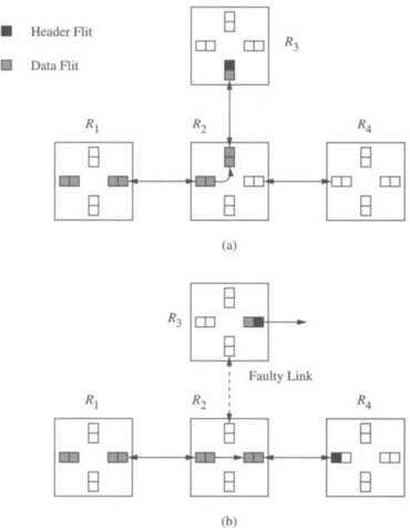
Figure 6.40 An example of flit-level copying and forwarding for exactly-once message delivery: (a) state of the routers prior to link failure and (b) state of the routers two cycles later, after a link failure has been detected.
Each message is comprised of four components: a header, tail, data, and the token signifying the end of the message. Figure 6.40(a) shows the state of a message just prior to failure of the link. Now assume that a link failure has been detected. Figure 6.40(b) shows the state of the routers two cycles later. One side of the failed link has the header and a single data flit. A token is generated (not shown), appended to the data flit, and this new message can now continue toward the destination. The data flits on the other side of the fault are orphaned. A new header is constructed, prepended to the first data flit, and routed as a new message. The token of the original message serves as the token for this message. Header reconstruction is supported by maintaining a copy of the header in all of the routers with a data flit from the message (not shown in the figure). When the message token passes through the router, the copies of the header flit can be cleared. To facilitate reconstruction of the message at the destination, the headers are distinguished (original and restart) as are the token types (unique and replica). Finally, although not shown, a copy of every flit is maintained on both sides of a link. Flit-level flow control must enable the correct release of flit copies. Whenever router R2 successfully transmits a flit to router R3, a copied signal is transmitted to R1 so that R1 may invalidate its copy of the flit. In this way exactly two copies of each data flit are maintained in the network at all times. A more detailed description of the architecture of the router implementation can be found in Chapter 7.
6.7.3 Message-Level Recovery
An alternative to flit-level recovery is to find and discard the interrupted message components and retransmit the message from the source. Recovery is at the level of complete messages rather than at the flit level. The PCS-based solutions exploit the fact that a separate control network comprised of the control channels exists. Consider a message pipeline where a fault is detected on a reserved virtual link or physical channel as shown in Figure 6.39. The link is marked faulty. The link controller at the source end of the faulty virtual link introduces a release flit (referred to as kill flit in [123]) into the complementary virtual control channel of the virtual link upstream from the fault. This release flit is routed back to the source router. The link controller at the destination end of the faulty virtual link introduces a release flit into the corresponding virtual control channel of the virtual link downstream from the failed virtual link. This release flit is propagated along toward the destination. When a release flit arrives at a node, the input and output virtual links associated with the message are released, and the flit is propagated toward the source (or destination). If multiple faults occur in one message pipeline, this mechanism is applied recursively to fault-free segments.
When a release flit arrives at an intermediate router node, the set of actions taken by that node will depend on the state of the interrupted message pipeline in that node. We have the following rules that are to be implemented by each router node. In all of the following steps it is implicit that virtual links and associated buffers are released. If two control flits for the same message arrive at a router node (from opposite directions along the path), the two control flits collide at that router node. A flit in progress toward the destination (source) is referred to as a forward (reverse) flit. The following rules govern the collision of control flits and are based on the assumption [123] that paths are removed by message acknowledgments from the destination rather than by the last flit of the message. Thus, a path is not removed until the last flit has been delivered to the destination. This behavior guarantees message delivery in the presence of dynamic or transient faults.
1. If a forward release flit collides with a reverse release flit, remove both release flits from the network. This may occur with multiple faults within the same message pipeline.
2. If a forward release flit collides with a message header (during the setup phase), remove both the routing header and the release flit.
3. If a release flit reaches the source, inform the message handler that the message transmission has failed. The handler may choose to retransmit or to invoke some higher-level fault-handling algorithm.
4. If a release flit reaches the destination, the partially received message is discarded.
5. If a forward release flit collides with a setup acknowledgment, the acknowledgment is removed from the network and the release flit is allowed to continue along the path toward the destination.
6. If a forward release flit collides with a message acknowledgment, both are removed from the network.
Release flits are injected into the network only on the occurrence of faults. Since faults are a dynamic phenomenon, they may occur at any time during path setup, message transmission, or message acknowledgment. The interaction of control flits produces the actions defined above to ensure proper recovery. In the fault-free case each virtual circuit contains at most one control flit at a time. Therefore, it is necessary to add additional buffer space for one reverse and one forward release flit per virtual control channel. Since nonheader control flits are allowed to pass blocked headers, release flits will not wait and therefore cannot create chains of blocked flits as shown in Figure 6.1. Header flits using backtracking PCS algorithms do not block on faults. Thus, no flit in the network blocks indefinitely on a fault. As a result, release flits cannot induce deadlock in the presence of faults, and the existing routing algorithm is deadlock-free.
As long as a path exists between the source and the destination, if a fault interrupts the message, both the source and the destination will be notified. However, it is possible that an inconsistent state can develop between a source and a destination where the destination has received the message intact, but the source believes the message was lost and must retransmit. This situation develops when a dynamic fault occurs in the virtual circuit after the last flit is delivered, but before the final message acknowledgment reaches the source. This situation can be remedied at the operating system level by assigning identification tags to messages. If the source is prevented from sending the next message until the previous message has been successfully received, the destination can detect and discard duplicate messages relatively easily.
The above approach requires the use of virtual channels to support recovery traffic. The use of virtual channels can complicate routing decisions and channel control, leading to an increase in the flow control latency through the router and across the channel. Fault-tolerant implementations of compressionless routing have been proposed [179], motivated by a desire to simplify router design to enable adaptive routing and fault recovery with speeds comparable to oblivious routers. Compressionless routing exploits the small amount of buffering within the network routers to be able to indirectly determine when the header of a message has reached the destination. For example, assume that each router can only buffer two flits at the input and output of a router. If a message is to traverse three routers to the destination, once the 12th flit has been injected into the network the source node can assert that the header has been received into the destination node queue. Figure 6.41 illustrates this case, with the exception that the message is actually comprised of 10 flits. When the last data flit is injected into the network, the header will not have reached the destination node. Therefore, the message is padded with pad flits. The number of pad flits that must be added is a function of the distance to the destination and the message size.
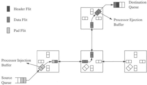
A separate pad signal enables the routers to distinguish between data flits and pad flits and is also used to remove the path when message transmission is complete. Thus, every message is padded with one pad flit as the tail flit. The pad signal appears as shown in Figure 6.42.
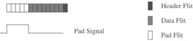
Fault-tolerant routing can now be realized as follows. The sender maintains a counter for the number of injected flits and a timer for recording the time a message remains blocked. The flit counter enables the sender to determine whether the header has reached the destination. For the static fault model, once the header flit has been delivered it can be asserted that the message will be delivered. If the header encounters a fault, it can be rerouted. Misrouting can be accommodated by limiting the number of nonminimal steps that are permitted and correspondingly increasing the number of required pad flits. No routing restrictions are enforced to prevent deadlock, and therefore routing is maximally adaptive. Rather, deadlock detection is employed. A timer is used to determine if a message has been blocked too long and is therefore possibly deadlocked. When the timer expires at the source, an FKILL control signal is transmitted from the source to release the path and buffers. The message is then retransmitted. Compressionless routing is based on the experimental observation that algorithms with a high degree of adaptivity rarely result in deadlocked message configurations. The occurrence of static faults is indistinguishable from deadlock due to cyclic dependencies.
In the case of dynamic faults, messages may be interrupted by faults, and therefore the algorithm requires some modification. Now messages are padded such that the path is held until the last data flit has reached the destination. If a fault interrupts a message in progress, the detecting router transmits FKILL and BKILL signals toward the destination and source routers, respectively, to release the path. When the destination receives an FKILL signal, it can be asserted that the received message is incomplete and can be discarded. The reception of a BKILL signal by the source causes retransmission by the source. Faults occurring on links that are transmitting pad flits do not require transmission of recovery signals.
Compressionless routing does not require virtual channels and is applicable to a wide variety of topologies. The KILL signals can be used for buffer allocation and for determining the immediate status of adaptively routed messages (i.e., whether they have been delivered or not). This latter property can be used to guarantee in-order delivery of multiple messages. The overall result is a simpler and therefore faster router design. However, pad flits use real bandwidth. If messages tend to be short and networks low dimensional and large, the increase in router speed is traded off against a drop in network utilization. An alternative view is that compressionless routing encourages the use of higher-dimensional networks with low average interprocessor distance.
6.7.4 Miscellaneous Issues
All of the approaches described in this section utilize bandwidth in different ways to enable recovery from dynamic faults and for synchronization between the source and destination to detect or avoid duplicate messages. These techniques do so while providing for fully distributed recovery of orphan flits. In PCS-based dynamic fault tolerance, network bandwidth is consumed by release flits and message acknowledgments for synchronization as well as recovery. In compressionless-routing-based recovery, network bandwidth is consumed by pad flits and a few extra control signals (which represent bandwidth that could otherwise have been used for data transmission). Exactly-once delivery appears to require the least amount of additional bandwidth for fault recovery at the expense of increased storage within the router. The increase in the number of messages produces an increase in the number of message headers. The headers utilize more bandwidth and storage within the routers for copies. However, with increasingly larger routers becoming feasible this does not appear to be a limiting factor. The increased message population changes the blocking probabilities experienced by all messages and can have some impact on average message latency and throughput. At low loads this impact would not appear to be significant.
Timeout mechanisms have been proposed for use at the link level as well as the message level. Link-level timeouts are often used to determine if flit transmission across a channel has been successful, and the timeout interval is generally easier to establish. Node-level timeouts have been used to determine if messages have been received. There are several issues with using timeouts at the node level. It is difficult to determine the appropriate value of the timeout interval since it is sensitive to traffic conditions and fault patterns. In the presence of dynamic communication traffic that varies across applications, conservative estimates of timeout intervals lead to long recovery times while small timeout intervals lead to false recovery; that is, network congestion is erroneously interpreted as a deadlock situation. Further, buffering requirements at the source node increase with the timeout interval since messages must be maintained for a longer period of time. Most importantly, the use of timeouts does not address the problem of recovering orphaned data flits in the network.
The availability of such distributed recovery mechanisms enables several existing adaptive routing algorithms based on wormhole switching to become fault recoverable. Consider fully adaptive routing algorithms under the wormhole switching model. Under the static fault model, if a wormhole-switched header blocks on a faulty virtual link, deadlock may occur. Thus, adaptive wormhole-switched routing algorithms that rely on deterministic subnetworks become deadlock-prone. If the header is forced to block waiting on a faulty link in a deterministic subnetwork, the recovery mechanism can be invoked to remove this message if recovery mechanisms are supported. Since the fault occurs at the location of the header flit, only the source node is informed that the route failed. The message may now be retransmitted or a higher-level fault handler may be invoked. Since the base routing algorithm is adaptive, a retransmitted message may possibly find a different path to the destination. However, since generally no memory of the past route is maintained, routing algorithms based on wormhole switching are likely to repeat their last route. Randomizing the choice of adaptive output channels will make these routing algorithms more robust. A final message acknowledgment is necessary to remove the message path and ensure delivery of the last flit.
6.8 Engineering Issues
The design of a reliable communication fabric arises naturally in the design of dependable systems. These emerging classes of systems can be relied upon to deliver services in the presence of failures. Attributes of dependable systems include availability, reliability, and security. Reliable interconnection networks form a natural component of such a system. For a given probability of failure for an isolated component, the probability of the failure of at least one component in a network grows as the size of the system increases. As described above, such failures can lead to deadlock, particularly in obliviously routed networks. Thus, the expectation is that dependable systems will incorporate some degree of fault-tolerant routing. The hard questions relate to the choice of technique and the cost/performance/reliability trade-offs.
The effective design of fault-tolerant networks must proceed from the initial specification of application requirements that specify system MTBF, acceptable message latency and network bandwidth, and system failure conditions. The application environment will determine the fault model. One effective methodology [154] proceeds from this point through a selection of fault-tolerant routing techniques and the establishment of fault tolerance/performance trade-offs, and culminates in the validation and verification of the design. Effective fault-tolerant network design requires that fault tolerance be considered from the outset and not added after a performance-based design.
The application requirements determine the fault model: the nature and the types of faults that can occur, their frequency of occurrence, and how they manifest themselves as errors. The routing algorithms described in this section assume that faults manifest themselves as failed links and routers. The pattern and rate of these failures depend on lower-level fault models that can be derived from the application requirements. For example, faults can be characterized as follows:
![]() Hard faults (e.g., radiation-induced, natural failures, etc.)
Hard faults (e.g., radiation-induced, natural failures, etc.)
![]() Transient faults (e.g., radiation-induced, switching transients, etc.)
Transient faults (e.g., radiation-induced, switching transients, etc.)
The specific faults and their manifestations (e.g., single-event upset and bit errors) must be derived from the target application environment. The description will include the rates at which these faults will occur and the requirements on MTTR, MTBF, acceptable degradation in message latency, and so on. These rates may vary by fault type. For example, soft faults may occur at different rates than hard faults. Soft faults can occur on the order of minutes to hours (e.g., in a space environment), while hard faults can occur on the order of months. One of the difficulties with establishing requirements is that they may also depend on the mode of operation. A system may move from operational to degraded mode after the occurrence of the first failure. The requirements on recovery latency may be more stringent in degraded mode. Requirements may be stronger during bursty traffic situations than under low-load conditions. Information from the application environment is used to establish the fault model and place constraints on fault recovery times.
Once the fault model has been established, decisions must be made on how the fault information is to be managed. Examples of alternatives include (1) the location and type of faults are globally known; (2) at each node, only the fault status of neighboring nodes are available; or (3) at each node the fault status of nodes within a k-distance neighborhood are known. The availability of global fault information will enable the computation and selection of optimal routes. The difficulty arises in the time and space overhead of maintaining this information and recomputing these global routes on-line. The use of global information also requires support for the reliable broadcast of fault information. This lengthens the recovery time, thus increasing the probability of the occurrence of a second fault before the system is finished recovering from the first. The use of purely local information enables fast rerouting decisions, but the lack of any form of lookahead can lead to network hot spots and resulting performance degradation. Natural trade-offs involve propagating fault information to a neighborhood and using this information in rerouting decisions.
Once the fault model and extent of fault location information has been determined, the major difficulty now is in choosing between the diverse set of fault-tolerant routing techniques. One set of guidelines can be obtained by considering the relationship between MTTR and MTBF as illustrated in Figure 6.43. Consider the case where MTTR ![]() MTBF. In this case we would expect the probability of the failure of two network components in the repair interval to be fairly low. During this time it may be permissible for the network to operate with degraded latency/throughput characteristics. In fact, depending on the network load, performance may not even be significantly degraded. Many machines operating in a commercial environment share these characteristics where the MTTR is on the order of hours to days while the MTBF is on the order of months. In this case, software-based techniques for rerouting messages may be preferred. The emerging switch-based networks such as Myrinet [30] and TNet [155] appear to have these characteristics. The Myrinet network is in fact automatically configured based on routing packets that determine interconnection topology. This is feasible since failures are not occurring at a rapid rate. The software-based approaches have minimal impact on the router design: messages encountering faults are simply ejected to the messaging layer of the local node. Messages that do not encounter faults remain unaffected (there may be second-order effects due to increased traffic as a result of rerouted messages). However, in the presence of even a single fault the messages that do encounter this failed component experience significant increase in latency, more so than in corresponding hardware-implemented rerouting schemes.
MTBF. In this case we would expect the probability of the failure of two network components in the repair interval to be fairly low. During this time it may be permissible for the network to operate with degraded latency/throughput characteristics. In fact, depending on the network load, performance may not even be significantly degraded. Many machines operating in a commercial environment share these characteristics where the MTTR is on the order of hours to days while the MTBF is on the order of months. In this case, software-based techniques for rerouting messages may be preferred. The emerging switch-based networks such as Myrinet [30] and TNet [155] appear to have these characteristics. The Myrinet network is in fact automatically configured based on routing packets that determine interconnection topology. This is feasible since failures are not occurring at a rapid rate. The software-based approaches have minimal impact on the router design: messages encountering faults are simply ejected to the messaging layer of the local node. Messages that do not encounter faults remain unaffected (there may be second-order effects due to increased traffic as a result of rerouted messages). However, in the presence of even a single fault the messages that do encounter this failed component experience significant increase in latency, more so than in corresponding hardware-implemented rerouting schemes.
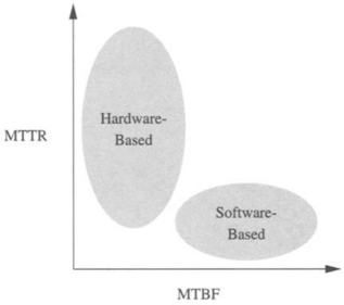
On the other hand, consider embedded systems with real-time requirements where MTTR ![]() MTBF. One such example is space-borne embedded computing systems, where repair is infeasible and therefore MTTR is effectively infinite. In this case an investment in hardware solutions may be justified. If we do consider hardware solutions, then the specific choice depends on the fault model. Packet switching and PCS in conjunction with backtracking and misrouting algorithms are the most robust and can tolerate large numbers of failures but extract both performance and cost overheads. The wormhole-switched routing algorithms based on block fault models are less expensive and simpler but are not as robust and require the construction of block fault regions. Both classes of solutions require custom routers. In addition to the probability of message delivery we must consider the impact on performance. Hardware solutions tend to provide better latency/throughput performance. Even a single fault leads to much higher message latencies for software-based rerouting. Thus, even if MTTR
MTBF. One such example is space-borne embedded computing systems, where repair is infeasible and therefore MTTR is effectively infinite. In this case an investment in hardware solutions may be justified. If we do consider hardware solutions, then the specific choice depends on the fault model. Packet switching and PCS in conjunction with backtracking and misrouting algorithms are the most robust and can tolerate large numbers of failures but extract both performance and cost overheads. The wormhole-switched routing algorithms based on block fault models are less expensive and simpler but are not as robust and require the construction of block fault regions. Both classes of solutions require custom routers. In addition to the probability of message delivery we must consider the impact on performance. Hardware solutions tend to provide better latency/throughput performance. Even a single fault leads to much higher message latencies for software-based rerouting. Thus, even if MTTR ![]() MTBF, performance constraints such as the need for real-time communication may favor hardware-based solutions.
MTBF, performance constraints such as the need for real-time communication may favor hardware-based solutions.
Between these two extremes (software versus custom hardware) there are compromise approaches that utilize some form of spatial and temporal redundancy with different trade-offs between cost and performance. For example, each message may be replicated and transmitted along a disjoint path through the network. The ability to route messages along disjoint paths requires source routing: the header contains the output port addresses of each intermediate router rather than the destination address or offset. A routing table at each source stores headers for each set of disjoint paths for every destination node. The design of these routing tables must be such that routing is guaranteed to be deadlock-free for multipacket transmission. This approach requires that routers be modified to be source routed (many commercial chips already are) and that network bandwidth be sacrificed for reliability. Sacrificing bandwidth may be feasible since most networks are usually limited by interface and software overheads rather than raw link bandwidths. The challenge here is creating routing tables that are deadlock-free in the presence of this style of traffic. Depending on the degree of replication (e.g., only two messages transmitted between nodes), recomputation of routing tables may be necessary if both paths are interrupted by a fault. Note that a message that cannot be delivered must be removed from the network to avoid deadlock. Other alternatives include dual redundant networks or routers. This is an expensive solution that may be infeasible in some environments due to cost or size, weight, or power constraints (e.g., embedded systems).
Many of the approaches described in this chapter rely on the absence of faults during some small interval of time during which system state is being updated (e.g., constructing block fault regions or updating routing tables). What happens if faults occur during this interval? What is the probability of such an occurrence? How do you make a choice between various approaches? Simulation-based modeling appears to be the approach of choice to evaluate the performance of these networks in pursuit of answers to these questions. It is useful to have tools that would permit empirical fault injection studies for a relatively more accurate analysis of the effect of faults and the ability of the system network to detect and respond to them in a timely fashion. Coverage analysis can be invaluable in designing the network. For example, fault injection studies can reveal the type of network error states that occur due to bit errors that corrupt the routing header. Tools such as DEPEND [339] can be used to utilize fault dictionaries that capture the manner in which errors are manifested due to various types of faults. These fault dictionaries can be used in fault injection studies to evaluate alternatives for fault-tolerant routing. For example, by using realistic fault injection models the analysis may discover that software-based rerouting provides the same level of fault coverage as more expensive hardware-based schemes and with acceptable rerouting message latency.
Evaluation tools should extend the analysis to the impact of faults on the execution of application programs. Reliable communications is a means to enable the execution of application programs. The primary consideration in the design of the network is the effect of faults and the fault-tolerant routing techniques on the execution of programs. In the presence of faults, message delivery may no longer be guaranteed. In this case the program execution may fail. Delivery probabilities can be estimated via simulation driven by communication traces of application programs or representative kernels. Formal models can also establish the ability of routing algorithms to find paths based on a known and fixed number or pattern of faults (e.g., up to the node degree). Most routing algorithms attempt to at least guarantee delivery when the number of faulty components is less than the node degree of the interconnection network.
A second effect of faults is on message latency, which is more of a concern in real-time systems. Virtual channels can have a significant impact on message latency. The failure of routers and links produces congestion in their vicinity as messages are rerouted. These messages will experience increased blocking delays as they compete for access to a smaller number of links. The presence of virtual channels will reduce the blocking delay and increase the overall network throughput. With backtracking routing algorithms, the presence of additional virtual channels affects the probability that a message is delivered since these algorithms do not block on busy channels. Thus, while studies have shown that the presence of virtual channels can affect the flow control latency through the routers, in the presence of faults they can have a substantial positive effect on latency.
The execution time performance of faulty networks depends on whether the network is operating at saturation, in the low-load region, or just at the brink of saturation. The performance/reliability trade-offs tend to be different for each operating region. The intuitive explanation follows from the fact that the message population consists of two types of messages: those that have encountered faults and those that have not. Consider operation with message destinations uniformly distributed in a mesh network. When operating in the low-load region, increasing the injection rate for a fixed number of faults may not significantly change the percentage of messages that encounter a faulty component. Thus, average latencies may not appear to be affected as the load increases. However, as we get closer to saturation the effects start to become more pronounced as congestion in the vicinity of faults makes the performance sensitive to the number of available channels and the use of oblivious or adaptive routing. Alternatively, for a fixed injection rate, as we increase the number of faults, the performance characteristics depend upon the routing techniques. With the use of software-based rerouting and a base oblivious routing algorithm, performance is significantly affected with each additional failure since a greater percentage of the message population encounters faulty components. However, adaptively routed networks will observe little change in message characteristics since the network initially has enough redundant bandwidth. As injection rates approach those corresponding to saturation, the occurrence of additional faults has a substantial impact on performance. For a fixed number of faults, when the network is in saturation the performance is dominated by the steady-state behavior of the messages that do not encounter faults. Each additional fault increases the percentage of the message population that has to be rerouted, contributing to congestion and further degradation in performance. The performance also depends on the buffering available at the individual nodes. These buffers provide a natural throttling mechanism and in effect control the saturation behavior of the network.
The difficulty is in determining the operating region for a set of applications. One way of deriving these requirements from an application is by developing an injection model that specifies the size of messages and the rate at which nodes can be expected to inject these messages into the network. This model is essentially a profile of the communication demands to be placed on the network. From this profile you can construct models to determine the demand on the bisection bandwidth and the demand on network bandwidth in general (see Chapter 9 for examples of how to specify performance in a topology-independent manner). From the injection model and physical network characteristics we can make some assessment of what region the network is operating in for the target applications. The injection model will depend on the processor speeds, the average number of instructions between communication commands, and the internal node bandwidth to the network interface.
A critical issue that has not been addressed in this chapter is fault detection. Although it is beyond the scope of this book, a few general points can be made. General fault tolerance and digital systems techniques are applicable within the routers, interfaces, and software layers. These detection mechanisms identify failed links or routers in keeping with the fault models for networks used here. In addition, link failures can be detected either by adding some redundant information in every transmission, by exercising some tests while the link is idle, or both. Adding redundant information requires a few additional wires per link. In the simplest case, a parity bit requires a single wire. However, this method allows the immediate detection of permanent as well as transient faults. As transient faults are more frequent in many designs, a simple algorithm may allow the retransmission of the information. On the other hand, testing idle links does not require additional wires (the receiving node retransmits the information back to the sender). Using otherwise idle bandwidth in this fashion permits a wider range of tests and consequently a more detailed analysis of link behavior. However, it does not detect the transmission of incorrect (i.e., corrupted) data. Both techniques complement each other very well. Other common techniques include protecting the packet header, data, or both with cyclic redundancy checks. By recomputing the checks for packets on the fly as they pass through a node it is possible to detect failed links. Phits traversing a channel can also be encoded to transmit error detection patterns. More extensive use of coding can correct certain classes of errors. Hard errors such as link failures or router failures are usually detected with timeouts. Similar techniques are also used for end-to-end flow control by using positive acknowledgments with timeouts, although in this case it may not be possible to determine the location of the failure.
Although the majority of proposals for fault-tolerant routing algorithms consider static faults, faults may occur at any time in real systems. Designers must consider handling dynamic faults. When a fault interrupts a message in transit, the message cannot be delivered, and a fragment of the message may remain in the network indefinitely, leading to deadlock. Support for dynamic faults must perform two different actions: removal of fragments of interrupted messages and notification of the source and destination nodes that message delivery has failed, thereby permitting retransmission and reception of the complete message. The latter action can be supported at higher-level protocol layers by message sizes in the header, message-level acknowledgments, and retransmission on failures. Router nodes then simply have to discard fragments of interrupted messages. The alternative is hardware support for recovery, usually by transmitting control information toward the destination and source nodes from the location of the fault. Such an approach does create some nontrivial synchronization problems (e.g., preventing the notification from overtaking the message header). Solutions have been proposed for these problems but do exact some costs in hardware implementation. Adding support to remove fragments of interrupted messages is very convenient because it does not slow down normal operation significantly (as opposed to retransmission based on higher-level protocols) and deadlocks produced by interrupted messages are avoided. However, notifying the source node produces an extra use of resources for every transmitted message, therefore degrading performance significantly even in the absence of faults. Considering the probability of interrupted messages, a trade-off must be made between the probability of dropping packets versus loss in performance.
Finally, if the network is designed to operate in an unattended environment, repair is not possible. In addition to selecting an appropriate switching technique and routing algorithm to meet the requirements on MTBF, it is useful for the network to be designed with higher numbers of dimensions. This will increase the number of disjoint paths between processors. The degradation in latency/throughput performance is expected to occur at a slower rate with a higher number of dimensions, increasing the likelihood of meeting requirements for a longer period of time.
6.9 Commented References
The notion of fault-tolerant routing has existed as long as there have been communication networks. In the context of multiprocessors some of the early work was naturally based on the early switching techniques, packet switching and circuit switching. While there has been a substantial amount of work in fault tolerance in indirect networks, this text has largely concentrated on the emerging systems using direct networks.
As direct-network-based multiprocessors evolved based on binary hypercubes, substantial analysis focused on the properties of this network. This topology was highly popular until low-dimensional networks became the topology of choice. A great deal of the analysis for fault tolerance focused on the connectivity properties of the binary hypercube in the presence of faults as opposed to the development of deadlock- and livelock-free routing algorithms. Thus, much of that literature has been omitted from this text in favor of what we hope are a few representative examples of routing techniques in faulty networks. In packet-switched binary hypercube networks, fault-tolerant routing algorithms tended to either exploit the unique topological properties of hypercubes or employ some form of graph search. For example, Chen and Shin used the concept of spare dimensions [53] to route around faulty regions. The spare dimension transported the message in a direction “orthogonal” to the faulty node. Routing was based on purely local information about the fault status of the neighboring nodes. Lee and Hayes [198] extended the state designation of a node to include the unsafe state. The unsafe state was used to serve as a warning that messages may become trapped or delayed if routed via nodes marked as unsafe. Lee and Hayes demonstrated that this approach can be used in the formulation of deadlock-free, wormhole-switched routing algorithms. Other routing algorithms followed that found ways to utilize the unsafe designation effectively, as well as extending the binary safe/unsafe designation to the notion of a range of safety levels [351].
The use of graph search techniques also led to the design of many adaptive fault-tolerant SAF routing algorithms. The critical issue here was how the state of the search was maintained and utilized to avoid repeated searches as well as the discovery of a path if one existed. Different techniques for maintaining the state of the network led to different routing algorithms, each exploiting the multidimensional structure of the hypercube in a different way. The Jet Propulsion Laboratory (JPL) Mark III hypercube [62] supported multiple modes of communication including both circuit switching and packet switching. Both modes operated with path setup following a best-first heuristic search for finding a path through the network around congested or faulty nodes. Chen and Shin [52] proposed a strategy that relied on a depth-first search of the network. In contrast to organized search, randomization was proposed as a deadlock avoidance technique for adaptive fault-tolerant routing [34, 188]. Messages can be adaptively routed, and when blocking occurs a randomly chosen message is misrouted. The formal analysis ensures that infinite paths are avoided and the messages are not indefinitely blocked. Simulation studies establish that adaptive routing is a viable approach toward avoiding faulty components. However, messages can still be completely buffered within a node. The use of small buffers in wormhole switching creates a new set of problems.
The first algorithms based on wormhole switching focused on fault regions that were convex and block structured, marking fault-free nodes as faulty if necessary. Messages could be routed around faulty regions without introducing cyclic dependencies with the aid of virtual channels—often organized explicitly as fault rings [37]—or by restricting adaptivity [58]. Both oblivious as well as adaptive routing algorithms could be adapted to this fault model. Subsequent work relaxed constraints on the location and relationship between fault regions. The basic principle underlying these approaches was to establish the minimal number of virtual networks necessary to separate traffic along the links. Traffic was usually characterized by the relationship between the source and destination by direction of traversal along each dimension. If message flows around a fault region could be separated and prevented from interacting, then routing could remain deadlock-free. A similar thought process has extended this approach to routing around certain classes of nonconvex fault regions [50].
While the preceding techniques used virtual channels, there was increasing interest in techniques for fault-tolerant routing using wormhole switching without the overhead of virtual channels. The turn model was extended to enable messages to be routed around faults by relying on a local relabeling scheme in the vicinity of faults [131]. Origin-based routing in meshes was also introduced for this purpose and is a generalization of turn model routing [145]. Messages are first routed toward the origin and then toward the destination. By placing the origin at different places within the mesh, messages could be routed around fault-free regions in a deadlock-free manner without the aid of virtual channels, although there are some constraints on the relative locations of fault regions.
More recent algorithms attempt to combine the flexibility of circuit-switched routing algorithms and wormhole-switched routing algorithms by using PCS switching and its variants [79, 126]. The resulting misrouting backtracking algorithms have fault tolerance properties similar to their packet-switched counterparts, but the performance is substantially better due to the pipelined data flow, particularly for large messages. While these approaches do not rely on virtual channels, they do rely on the availability of a distinct control channel across each physical channel.
All of the approaches described here assume the implementation of routing and selection functions within the network routers to implement the fault-tolerant routing algorithms, resulting in expensive custom solutions. Suh et al. [333] point out that in some low-fault-rate environments, software-based rerouting is a viable option when repair times are short relative to network component MTBF. The network can operate in degraded mode until repair. The challenge here is devising rerouting strategies that are deadlock- and livelock-free in the presence of a wide range of fault patterns. Certain pathological fault patterns may pose a problem while exhaustive search techniques may still find paths. It is interesting to note that such a strategy also accommodates a wider range of fault patterns for both adaptive and oblivious routing; however, the performance penalty for rerouted messages is high.
Finally while rerouting is acceptable for statically known component failures, the occurrence of failures that disrupt messages necessitates recovery mechanisms. Two very similar techniques include compressionless routing [179] and acknowledged PCS [123]. Both recover messages in a distributed fashion although they use network bandwidth in different ways. The Reliable Router from MIT has an exactly-once delivery philosophy [74]. Interrupted messages form smaller messages that are independently routed through the network to their destinations. No retransmission is involved. In general, these recovery mechanisms can complement any one of the existing routing algorithms based on pipelined switching mechanisms. We can now expect to see techniques evolve that will accommodate collective communication operations, and we can expect to see irregular topologies that will be designed for the clustered workstation environment.
Exercises
6.1. Show that for dimension-order routing in a 2-D mesh, only two virtual channels are required for routing around rectangular fault regions with nonoverlapping fault rings. How would this change if fault rings are allowed to overlap?
Solution Figure 6.44 illustrates the routing restrictions necessary for deadlock-free routing [37]. Since messages traveling in the horizontal dimension and messages traveling in the vertical dimension use a distinct set of channels, deadlock can only occur due to cyclic dependencies between messages within each group (i.e., horizontal or vertical). From the figure we see that eastbound and westbound messages always traverse a disjoint set of c0 channels. Thus, they do not interfere with each other. Since the topology is a mesh and there are no wraparound channels, there are no cyclic dependencies between c0 channels. Now consider the northbound and southbound messages that use the c1 channels. Note that these messages are restricted to following a clockwise or counterclockwise orientation around the fault regions. Thus, a message in one group cannot block on a channel held by a message in the other group. In the absence of wraparound channels, northbound and southbound messages do not form cyclic channel dependencies. Thus, the solution shown in the figure is deadlock-free.
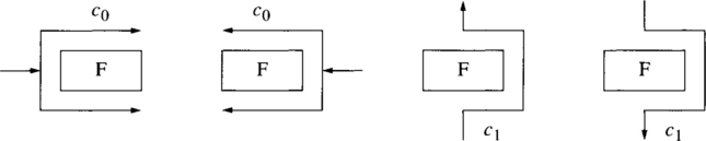
Now if fault rings were allowed to overlap, the eastbound messages traversing a fault region in the clockwise direction may share a channel with (and therefore block) a message traversing an adjacent fault region in the counterclockwise direction. Thus, eastbound and westbound messages can form cyclic dependencies. The solution is to introduce additional virtual channels to further separate the traffic on a link. Two additional virtual channels per link will suffice.
6.2. Consider a k-ary n-cube network with f faults. What is the maximum number of consecutive links that a PCS header will have to backtrack in any single source/destination path?
Solution If there have been no previous misroutes, the header flit is allowed to misroute in the presence of faults even when the number of misroutes is limited. Thus, the header will only backtrack when the only healthy channel is the one previously used to reach the node. In the case of a k-ary n-cube, every node has 2n channels incident on a distinct node. Since the header arrived from a nonfaulty node, it will be forced to backtrack if (2n − 1) channels are faulty. At the next node, since the header has backtracked from a nonfaulty node and originally arrived from a nonfaulty node, it will be forced to backtrack if the remaining (2n − 2) channels are faulty. Each additional backtracking step will be forced by (2n − 2) additional failed channels. Thus we have:
6.3. Now consider a multidimensional mesh-connected network with a backtracking, misrouting, packet-switched routing algorithm. What is the maximum number of consecutive links that the message will backtrack in the presence of f faulty links or nodes?
Solution If there have been no previous misrouting operations, the message is allowed to misroute in the presence of faults, even if the maximum number of misrouting operations is limited. There are several possible cases:
1. The routing probe is at a node with 2n channels. This is the same case as with a torus-connected k-ary n-cube. Hence, the number of faults required to force the first backtrack is (2n − 1). To force additional backtracks, (2n − 2) additional faults are required per additional backtrack.
2. The probe is at a node with less than 2n channels. As with the earlier cases, all channels except the one used to reach the node can be used in case of faults (either for routing or misrouting). The worst case occurs when the node has the minimum number of channels. In an n-dimensional mesh, nodes located at the corners only have n channels. One of the channels was used by the probe to reach the node. Hence, the failure of (n − 1) channels or nodes causes the routing probe to backtrack. The probe is now on the edge of the mesh, where each node has (n + 1) channels. One channel was already used to reach the node the first time and another one for the previous backtracking operation; therefore, only (n − 1) channels are available for routing. These channels must all be faulty to force a backtrack operation. Thus, the maximum number of mandatory backtrack operations is  .
.
3. The probe made a turn from a corner into a dead end. In order to cause the initial backtrack, there need to be n faults. (n − 2) faults are required to cause a backtrack at the corner node. Each additional backtrack requires (n − 1) faults. Hence, the maximum number of backtracking operations is ⌊(f + 1)/(n − 1)⌋.
6.4. In a binary hypercube with N = 2n nodes, a list of dimensions that have been traversed by a message is given as [1, 3, 6, 2, 3, 1, 5] and a current intermediate node as 24. An outgoing link across dimension 4 is a candidate output link for this message. Has this node been visited by this message?
Solution By reversing the coordinate sequence we can reconstruct the sequence of nodes that has been visited by this message. The previous node is given by 0011000 ![]() 010000 = 0111000 = node 56. The other nodes on the path include 58, 50, 54, 118, 126, and 124.
010000 = 0111000 = node 56. The other nodes on the path include 58, 50, 54, 118, 126, and 124.
Problems
6.1. In a binary hypercube with N = 2n nodes, how many shortest paths are affected by the failure of a single link?
6.2. Modify DP to permit misrouting in any dimension lower than the last dimension traversed in the escape network. Show that such an algorithm can tolerate all single-node or single-link faults except in the last dimension.
6.3. Consider the use of fault rings for fault-tolerant oblivious routing in 2-D meshes using four virtual channels per link. Fault rings may overlap. Draw the channel dependencies between the input virtual channels and output virtual channels at a router node.
6.4. Consider a k-ary n-cube network with f faults. What is the maximum number of consecutive links that a PCS header will have to backtrack in any single source/destination path?
6.5. Show that with at most three faulty components e-sft is livelock-free. With such a small number of components, you can ignore the PF flag.
6.6. The negative-first or north-last turn model routing algorithms have limited adaptivity for some source/destination pairs, and therefore are deadlock-prone without fault recovery. Combine two turn model routing algorithms to produce a fully adaptive fault-tolerant routing algorithm.
Hint Use distinct virtual networks. Specify constraints on the traversal of a message between networks to realize deadlock freedom.
6.7. Consider the fault regions shown in Figure 6.45 in a 2-D mesh. Show the channels used by EW, WE, NS, and SN meshes assuming dimension-order routing. The purpose of this exercise is to be able to observe that each group of messages utilizes a disjoint set of channels, and that the channel dependencies within each group are acyclic.
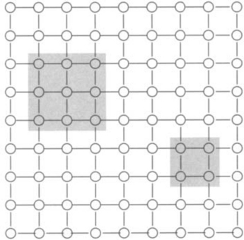
6.8. Given the location of the origin as shown in Figure 6.46, identify the possible paths taken by a message from the source (S) to each of the destinations, D1, D2, and D3, in origin-based routing.

6.9. Show how you can include fault recovery to make the routing algorithm of Dally and Aoki [73] deadlock-free in the presence of faults.
6.10. In a k-ary n-cube with f <2n faults, what is the maximum path length of a packet-switched message routed using an algorithm that permits a maximum of m misroutes?
6.11. Consider a routing algorithm in binary hypercubes where the dimensions to be traversed by a message are partitioned into two groups—the set of UP dimensions (the 0 → 1 direction across a dimension) and the set of DOWN dimensions. Routing proceeds by routing across UP dimensions in any order and across DOWN dimensions in strictly dimension order. What is the maximum number of faults that can be tolerated by adaptively routing in this fashion?