Introduction
Interconnection networks are currently being used for many different applications, ranging from internal buses in very large-scale integration (VLSI) circuits to wide area computer networks. Among others, these applications include backplane buses and system area networks; telephone switches; internal networks for asynchronous transfer mode (ATM) and Internet Protocol (IP) switches; processor/memory interconnects for vector supercomputers; interconnection networks for multicomputers and distributed shared-memory multiprocessors; clusters of workstations and personal computers; local area networks; metropolitan area networks; wide area computer networks; and networks for industrial applications. Additionally, the number of applications requiring interconnection networks is continuously growing. For example, an integral control system for a car requires a network connecting several microprocessors and devices.
The characteristics and cost of these networks depend considerably on the application. There are no general solutions. For some applications, interconnection networks have been studied in depth for decades. This is the case for telephone networks, computer networks, and backplane buses. These networks are covered in many books. However, there are some other applications that have not been fully covered in the existing literature. This is the case for the interconnection networks used in multicomputers and distributed shared-memory multiprocessors.
The lack of standards and the need for very high performance and reliability pushed the development of interconnection networks for multicomputers. This technology was transferred to distributed shared-memory multiprocessors, improving the scalability of those machines. However, distributed shared-memory multiprocessors require an even higher network performance than multicomputers, pushing the development of interconnection networks even more. More recently, this network technology began to be transferred to local area networks (LANs). Also, it has been proposed as a replacement for backplane buses, creating the concept of a system area network (SAN). Hence, the advances in interconnection networks for multicomputers are the basis for the development of interconnection networks for other architectures and environments. Therefore, there is a need for structuring the concepts and solutions for this kind of interconnection network. Obviously, when this technology is transferred to another environment, new issues arise that have to be addressed.
Moreover, several of these networks are evolving very quickly, and the solutions proposed for different kinds of networks are overlapping. Thus, there is a need for formally stating the basic concepts, the alternative design choices, and the design trade-offs for most of those networks. In this book, we take that challenge and present in a structured way the basic underlying concepts of most interconnection networks, as well as the most interesting solutions currently implemented or proposed in the literature. As indicated above, the network technology developed for multicomputers has been transferred to other environments. Therefore, in this book we will mainly describe techniques developed for multicomputer networks. Most of these techniques can also be applied to distributed shared-memory multiprocessors and to local and system area networks. However, we will also describe techniques specifically developed for these environments.
1.1 Parallel Computing and Networks
The demand for even more computing power has never stopped. Although the performance of processors has doubled in approximately every three-year span from 1980 to 1996, the complexity of the software as well as the scale and solution quality of applications have continuously driven the development of even faster processors. A number of important problems have been identified in the areas of defense, aerospace, automotive applications, and science, whose solutions require a tremendous amount of computational power. In order to solve these grand challenge problems, the goal has been to obtain computer systems capable of computing at the teraflops (1012 floating-point operations per second) level. Even the smallest of these problems requires gigaflops (109 floating-point operations per second) of performance for hours at a time. The largest problems require teraflops performance for more than a thousand hours at a time.
Parallel computers with multiple processors are opening the door to teraflops computing performance to meet the increasing demand of computational power. The demand includes more computing power, higher network and input/output (I/O) bandwidths, and more memory and storage capacity. Even for applications requiring a lower computing power, parallel computers can be a cost-effective solution. Processors are becoming very complex. As a consequence, processor design cost is growing so fast that only a few companies all over the world can afford to design a new processor. Moreover, design cost should be amortized by selling a very high number of units. Currently, personal computers and workstations dominate the computing market. Therefore, designing custom processors that boost the performance one order of magnitude is not cost-effective. Similarly, designing and manufacturing high-speed memories and disks is not cost-effective. The alternative choice consists of designing parallel computers from commodity components (processors, memories, disks, interconnects, etc.). In these parallel computers, several processors cooperate to solve a large problem. Memory bandwidth can be scaled with processor computing power by physically distributing memory components among processors. Also, redundant arrays of inexpensive disks (RAID) allow the implementation of high-capacity reliable parallel file systems meeting the performance requirements of parallel computers.
However, a parallel computer requires some kind of communication subsystem to interconnect processors, memories, disks, and other peripherals. The specific requirements of these communication subsystems depend on the architecture of the parallel computer. The simplest solution consists of connecting processors to memories and disks as if there were a single processor, using system buses and I/O buses. Then, processors can be interconnected using the interfaces to local area networks. Unfortunately, commodity communication subsystems have been designed to meet a different set of requirements, that is, those arising in computer networks. Although networks of workstations have been proposed as an inexpensive approach to build parallel computers, the communication subsystem becomes the bottleneck in most applications.
Therefore, designing high-performance interconnection networks becomes a critical issue to exploit the performance of parallel computers. Moreover, as the interconnection network is the only subsystem that cannot be efficiently implemented by using commodity components, its design becomes very critical. This issue motivated the writing of this book. Up to now, most manufacturers designed custom interconnection networks (nCUBE-2, nCUBE-3, Intel Paragon, Cray T3D, Cray T3E, Thinking Machines Corp. CM-5, NEC Cenju-3, IBM SP2). More recently, several high-performance switches have been developed (Autonet, Myrinet, ServerNet) and are being marketed. These switches are targeted to workstations and personal computers, offering the customer the possibility of building an inexpensive parallel computer by connecting cost-effective computers through high-performance switches. The main issues arising in the design of networks for both approaches are covered in this book.
1.2 Parallel Computer Architectures
In this section, we briefly introduce the most popular parallel computer architectures. This description will focus on the role of the interconnection network. A more detailed description is beyond the scope of this book.
The idea of using commodity components for the design of parallel computers led to the development of distributed-memory multiprocessors, or multicomputers, in the early 1980s. These parallel computers consist of a set of processors, each one connected to its own local memory. Processors communicate between themselves by passing messages through an interconnection network. Figure 1.1(a) shows a simple scheme for this architecture. The first commercial multicomputers utilized commodity components, including Ethernet controllers to implement communication between processors. Unfortunately, commodity communication subsystems were too slow, and the interconnection network became the bottleneck of those parallel computers. Several research efforts led to the development of interconnection networks that are several orders of magnitude faster than Ethernet networks. Most of the performance gain is due to architectural rather than technological improvements.
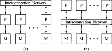
Figure 1.1 Schematic representation of parallel computers: (a) a multicomputer and (b) a UMA shared-memory multiprocessor. (M = memory; P = processor.)
Programming multicomputers is not an easy task. The programmer has to take care of distributing code and data among the processors in an efficient way, invoking message-passing calls whenever some data are needed by other processors. On the other hand, shared-memory multiprocessors provide a single memory space to all the processors, simplifying the task of exchanging data among processors. Access to shared memory has been traditionally implemented by using an interconnection network between processors and memory (Figure 1.1(b)). This architecture is referred to as uniform memory access (UMA) architecture. It is not scalable because memory access time includes the latency of the interconnection network, and this latency increases with system size.
More recently, shared-memory multiprocessors followed some trends previously established for multicomputers. In particular, memory has been physically distributed among processors, therefore reducing the memory access time for local accesses and increasing scalability. These parallel computers are referred to as distributed shared-memory multiprocessors (DSMs). Accesses to remote memory are performed through an interconnection network, very much like in multicomputers. The main difference between DSMs and multicomputers is that messages are initiated by memory accesses rather than by calling a system function. In order to reduce memory latency, each processor has several levels of cache memory, thus matching the speed of processors and memories. This architecture provides nonuniform memory access (NUMA) time. Indeed, most of the nonuniformity is due to the different access time between caches and main memories, rather than the different access time between local and remote memories. The main problem arising in DSMs is cache coherence. Several hardware and software cache coherence protocols have been proposed. These protocols produce additional traffic through the interconnection network.
The use of custom interconnects makes multicomputers and DSMs quite expensive. So, networks of workstations (NOWs) have been proposed as an inexpensive approach to build parallel computers. NOWs take advantage of recent developments in LANs. In particular, the use of ATM switches has been proposed to implement NOWs. However, ATM switches are still expensive, which has motivated the development of high-performance switches, specifically designed to provide a cost-effective interconnect for workstations and personal computers.
Although there are many similarities between interconnection networks for multicomputers and DSMs, it is important to keep in mind that performance requirements may be very different. Messages are usually very short when DSMs are used. Additionally, network latency is important because memory access time depends on that latency. However, messages are typically longer and less frequent when using multicomputers. Usually the programmer is able to adjust the granularity of message communication in a multicomputer. On the other hand, interconnection networks for multicomputers and NOWs are mainly used for message passing. However, the geographical distribution of workstations usually imposes constraints on the way processors are connected. Also, individual processors may be connected to or disconnected from the network at any time, thus imposing additional design constraints.
1.3 Network Design Considerations
Interconnection networks play a major role in the performance of modern parallel computers. There are many factors that may affect the choice of an appropriate interconnection network for the underlying parallel computer. These factors include the following:
1. Performance requirements. Processes executing in different processors synchronize and communicate through the interconnection network. These operations are usually performed by explicit message passing or by accessing shared variables. Message latency is the time elapsed between the time a message is generated at its source node and the time the message is delivered at its destination node. Message latency directly affects processor idle time and memory access time to remote memory locations. Also, the network may saturate–it may be unable to deliver the flow of messages injected by the nodes, limiting the effective computing power of a parallel computer. The maximum amount of information delivered by the network per time unit defines the throughput of that network.
2. Scalability. A scalable architecture implies that as more processors are added, their memory bandwidth, I/O bandwidth, and network bandwidth should increase proportionally. Otherwise the components whose bandwidth does not scale may become a bottleneck for the rest of the system, decreasing the overall efficiency accordingly.
3. Incremental expandability. Customers are unlikely to purchase a parallel computer with a full set of processors and memories. As the budget permits, more processors and memories may be added until a system’s maximum configuration is reached. In some interconnection networks, the number of processors must be a power of 2, which makes them difficult to expand. In other cases, expandability is provided at the cost of wasting resources. For example, a network designed for a maximum size of 1,024 nodes may contain many unused communication links when the network is implemented with a smaller size. Interconnection networks should provide incremental expandability, allowing the addition of a small number of nodes while minimizing resource wasting.
4. Partitionability. Parallel computers are usually shared by several users at a time. In this case, it is desirable that the network traffic produced by each user does not affect the performance of other applications. This can be ensured if the network can be partitioned into smaller functional subsystems. Partitionability may also be required for security reasons.
5. Simplicity. Simple designs often lead to higher clock frequencies and may achieve higher performance. Additionally, customers appreciate networks that are easy to understand because it is easier to exploit their performance.
6. Distance span. This factor may lead to very different implementations. In multicomputers and DSMs, the network is assembled inside a few cabinets. The maximum distance between nodes is small. As a consequence, signals are usually transmitted using copper wires. These wires can be arranged regularly, reducing the computer size and wire length. In NOWs, links have very different lengths and some links may be very long, producing problems such as coupling, electromagnetic noise, and heavy link cables. The use of optical links solves these problems, equalizing the bandwidth of short and long links up to a much greater distance than when copper wire is used. Also, geographical constraints may impose the use of irregular connection patterns between nodes, making distributed control more difficult to implement.
7. Physical constraints. An interconnection network connects processors, memories, and/or I/O devices. It is desirable for a network to accommodate a large number of components while maintaining a low communication latency. As the number of components increases, the number of wires needed to interconnect them also increases. Packaging these components together usually requires meeting certain physical constraints, such as operating temperature control, wiring length limitation, and space limitation. Two major implementation problems in large networks are the arrangement of wires in a limited area and the number of pins per chip (or board) dedicated to communication channels. In other words, the complexity of the connection is limited by the maximum wire density possible and by the maximum pin count. The speed at which a machine can run is limited by the wire lengths, and the majority of the power consumed by the system is used to drive the wires. This is an important and challenging issue to be considered. Different engineering technologies for packaging, wiring, and maintenance should be considered.
8. Reliability and repairability. An interconnection network should be able to deliver information reliably. Interconnection networks can be designed for continuous operation in the presence of a limited number of faults. These networks are able to send messages through alternative paths when some faults are detected. In addition to reliability, interconnection networks should have a modular design, allowing hot upgrades and repairs. Nodes can also fail or be removed from the network. In particular, a node can be powered off in a network of workstations. Thus, NOWs usually require some reconfiguration algorithm for the automatic reconfiguration of the network when a node is powered on or off.
9. Expected workloads. Users of a general-purpose machine may have very different requirements. If the kind of applications that will be executed in the parallel computer are known in advance, it may be possible to extract some information on usual communication patterns, message sizes, network load, and so on. That information can be used for the optimization of some design parameters. When it is not possible to get information on expected workloads, network design should be robust; that is, design parameters should be selected in such a way that performance is good over a wide range of traffic conditions.
10. Cost constraints. Finally, it is obvious that the “best” network may be too expensive. Design decisions often are trade-offs between cost and other design factors. Fortunately, cost is not always directly proportional to performance. Using commodity components whenever possible may considerably reduce the overall cost.
1.4 Classification of Interconnection Networks
Among other criteria, interconnection networks have been traditionally classified according to the operating mode (synchronous or asynchronous) and network control (centralized, decentralized, or distributed). Nowadays, multicomputers, multiprocessors, and NOWs dominate the parallel computing market. All of these architectures implement asynchronous networks with distributed control. Therefore, we will focus on other criteria that are currently more significant.
A classification scheme is shown in Figure 1.2, which categorizes the known interconnection networks into four major classes based primarily on network topology: shared-medium networks, direct networks, indirect networks, and hybrid networks. For each class, the figure shows a hierarchy of subclasses, also indicating some real implementations for most of them. This classification scheme is based on the classification proposed in [253], and it mainly focuses on networks that have been implemented. It is by no means complete, as other new and innovative interconnection networks may emerge as technology further advances, such as mobile communication and optical interconnections.

Figure 1.2 Classification of interconnection networks. (Explanations of acronyms can be found in Appendix B.)
In shared-medium networks, the transmission medium is shared by all communicating devices. An alternative to this approach consists of having point-to-point links directly connecting each communicating device to a (usually small) subset of other communicating devices in the network. In this case, any communication between nonneighboring devices requires transmitting the information through several intermediate devices. These networks are known as direct networks. Instead of directly connecting the communicating devices between them, indirect networks connect those devices by means of one or more switches. If several switches exist, they are connected between them by using point-to-point links. In this case, any communication between communicating devices requires transmitting the information through one or more switches. Finally, hybrid approaches are possible. These network classes and the corresponding subclasses will be described in the following sections.
1.5 Shared-Medium Networks
The least complex interconnect structure is one in which the transmission medium is shared by all communicating devices. In such shared-medium networks, only one device is allowed to use the network at a time. Every device attached to the network has requester, driver, and receiver circuits to handle the passing of addresses and data. The network itself is usually passive, since the network itself does not generate messages.
An important issue here is the arbitration strategy that determines the mastership of the shared-medium network to resolve network access conflicts. A unique characteristic of a shared medium is its ability to support atomic broadcast, in which all devices on the medium can monitor network activities and receive the information transmitted on the shared medium. This property is important to efficiently support many applications requiring one-to-all or one-to-many communication services, such as barrier synchronization and snoopy cache coherence protocols. Due to limited network bandwidth, a single shared medium can only support a limited number of devices before the medium becomes a bottleneck.
Shared-medium networks constitute a well-established technology. Additionally, their limited bandwidth restricts their use in multiprocessors. So, these networks will not be covered in this book, but we will present a short introduction in the following sections. There are two major classes of shared-medium networks: local area networks, mainly used to construct computer networks that span physical distances no longer than a few kilometers, and backplane buses, mainly used for internal communication in uniprocessors and multiprocessors.
1.5.1 Shared-Medium Local Area Networks
High-speed LANs can be used as a networking backbone to interconnect computers to provide an integrated parallel and distributed computing environment. Physically, a shared-medium LAN uses copper wires or fiber optics in a bit-serial fashion as the transmission medium. The network topology is either a bus or a ring. Depending on the arbitration mechanism used, different LANs have been commercially available. For performance and implementation reasons, it is impractical to have a centralized control or to have some fixed access assignment to determine the bus master who can access the bus. Three major classes of LANs based on distributed control are described below.
Contention Bus
The most popular bus arbitration mechanism is to have all devices compete for the exclusive access right of the bus. Due to the broadcast nature of the bus, all devices can monitor the state of the bus, such as idle, busy, and collision. Here the term “collision” means that two or more devices are using the bus at the same time and their data collided. When the collision is detected, the competing devices will quit transmission and try later. The most well-known contention-based LAN is Ethernet, which adopts carrier-sense multiple access with collision detection (CSMA/CD) protocol. The bandwidth of Ethernet is 10 Mbits/s and the distance span is 250 meters (coaxial cable). As processors are getting faster, the number of devices that can be connected to Ethernet is limited to avoid the network bottleneck. In order to break the 10 Mbits/s bandwidth barrier, Fast Ethernet can provide 100 Mbits/s bandwidth.
Token Bus
One drawback of the contention bus is its nondeterministic nature as there is no guarantee of how much waiting time is required to gain the bus access right. Thus, the contention bus is not suitable to support real-time applications. To remove the nondeterministic behavior, an alternative approach involves passing a token among the network devices. The owner of the token has the right to access the bus. Upon completion of the transmission, the token is passed to the next device based on some scheduling discipline. By restricting the maximum token holding time, the upper bound that a device has to wait for the token can be guaranteed. Arcnet supports token bus with a bandwidth of 2.5 Mbits/s.
Token Ring
The idea of token ring is a natural extension of token bus as the passing of the token forms a ring structure. IBM token ring supports bandwidths of both 4 and 16 Mbits/s based on coaxial cable. Fiber Distributed Data Interface (FDDI) provides a bandwidth of 100 Mbits/s using fiber optics.
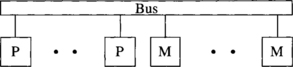
1.5.2 Shared-Medium Backplane Bus
A backplane bus is the simplest interconnection structure for bus-based parallel computers. It is commonly used to interconnect processor(s) and memory modules to provide UMA architecture. Figure 1.3 shows a single-bus network. A typical backplane bus usually has 50–300 wires and is physically realized by printed lines on a circuit board or by discrete (backplane) wiring. Additional costs are incurred by interface electronics, such as line drivers, receivers, and connectors.
There are three kinds of information in the backplane bus: data, address, and control signals. Control signals include bus request signal and request grant signal, among many others. In addition to the width of data lines, the maximum bus bandwidth that can be provided is dependent on the technology. The number of processors that can be put on a bus depends on many factors, such as processor speed, bus bandwidth, cache architecture, and program behavior.
Methods of Information Transfer
Both data and address information must be carried in the bus. In order to increase the bus bandwidth and provide a large address space, both data width and address bits have to be increased. Such an increase implies another increase in the bus complexity and cost. Some designs try to share address and data lines. For multiplexed transfer, addresses and data are sent alternatively. Hence, they can share the same physical lines and require less power and fewer chips. For nonmultiplexed transfer, address and data lines are separated. Thus, data transfer can be done faster.
In synchronous bus design, all devices are synchronized with a common clock. It requires less complicated logic and has been used in most existing buses. However, a synchronous bus is not easily upgradable. New faster processors are difficult to fit into a slow bus.
In asynchronous buses, all devices connected to the bus may have different speeds and their own clocks. They use a handshaking protocol to synchronize with each other. This provides independence for different technologies and allows slower and faster devices with different clock rates to operate together. This also implies buffering is needed, since slower devices cannot handle messages as quickly as faster devices.
Bus Arbitration
In a single-bus network, several processors may attempt to use the bus simultaneously. To deal with this, a policy must be implemented that allocates the bus to the processors making such requests. For performance reasons, bus allocation must be carried out by hardware arbiters. Thus, in order to perform a memory access request, the processor has to exclusively own the bus and become the bus master. To become the bus master, each processor implements a bus requester, which is a collection of logic to request control of the data transfer bus. On gaining control, the requester notifies the requesting master.
Two alternative strategies are used to release the bus:
![]() Release-when-done: release the bus when data transfer is done
Release-when-done: release the bus when data transfer is done
![]() Release-on-request: hold the bus until another processor requests it
Release-on-request: hold the bus until another processor requests it
Several different bus arbitration algorithms have been proposed, which can be classified into centralized or distributed. A centralized method has a central bus arbiter. When a processor wants to become the bus master, it sends out a bus request to the bus arbiter, which then sends out a request grant signal to the requesting processor. A bus arbiter can be an encoder-decoder pair in hardware design. In a distributed method, such as the daisy chain method, there is no central bus arbiter. The bus request signals form a daisy chain. The mastership is released to the next device when data transfer is done.
Split Transaction Protocol
Most bus transactions involve request and response. This is the case for memory read operations. After a request is issued, it is desirable to have a fast response. If a fast response time is expected, the bus mastership is not released after sending the request, and data can be received soon. However, due to memory latency, the bus bandwidth is wasted while waiting for a response. In order to minimize the waste of bus bandwidth, the split transaction protocol has been used in many bus networks.
In this protocol, the bus mastership is released immediately after the request, and the memory has to gain mastership before it can send the data. Split transaction protocol has a better bus utilization, but its control unit is much more complicated. Buffering is needed in order to save messages before the device can gain the bus mastership.
To support shared-variable communication, some atomic read/modify/write operations to memories are needed. With the split transaction protocol, those atomic operations can no longer be indivisible. One approach to solve this problem is to disallow bus release for those atomic operations.
Bus Examples
Several examples of buses and the main characteristics are listed below.
![]() Gigaplane used in Sun Ultra Enterprise X000 Server (ca. 1996): 2.68 Gbyte/s peak, 256 bits data, 42 bits address, split transaction protocol, 83.8 MHz clock.
Gigaplane used in Sun Ultra Enterprise X000 Server (ca. 1996): 2.68 Gbyte/s peak, 256 bits data, 42 bits address, split transaction protocol, 83.8 MHz clock.
![]() DEC AlphaServer8X00, that is, 8200 and 8400 (ca. 1995): 2.1 Gbyte/s, 256 bits data, 40 bits address, split transaction protocol, 100 MHz clock (1 foot length).
DEC AlphaServer8X00, that is, 8200 and 8400 (ca. 1995): 2.1 Gbyte/s, 256 bits data, 40 bits address, split transaction protocol, 100 MHz clock (1 foot length).
![]() SGI PowerPath-2 (ca. 1993): 1.2 Gbyte/s, 256 bits data, 40 bits address, 6 bits control, split transaction protocol, 47.5 MHz clock (1 foot length).
SGI PowerPath-2 (ca. 1993): 1.2 Gbyte/s, 256 bits data, 40 bits address, 6 bits control, split transaction protocol, 47.5 MHz clock (1 foot length).
![]() HP9000 Multiprocessor Memory Bus (ca. 1993): 1 Gbyte/s, 128 bits data, 64 bits address, 13 inches, pipelined bus, 60 MHz clock.
HP9000 Multiprocessor Memory Bus (ca. 1993): 1 Gbyte/s, 128 bits data, 64 bits address, 13 inches, pipelined bus, 60 MHz clock.
1.6 Direct Networks
Scalability is an important issue in designing multiprocessor systems. Bus-based systems are not scalable because the bus becomes the bottleneck when more processors are added.
The direct network or point-to-point network is a popular network architecture that scales well to a large number of processors. A direct network consists of a set of nodes, each one being directly connected to a (usually small) subset of other nodes in the network. Each node is a programmable computer with its own processor, local memory, and other supporting devices. These nodes may have different functional capabilities. For example, the set of nodes may contain vector processors, graphics processors, and I/O processors. Figure 1.4 shows the architecture of a generic node. A common component of these nodes is a router, which handles message communication among nodes. For this reason, direct networks are also known as router-based networks. Each router has direct connections to the router of its neighbors. Usually, two neighboring nodes are connected by a pair of unidirectional channels in opposite directions. A bidirectional channel may also be used to connect two neighboring nodes. Although the function of a router can be performed by the local processor, dedicated routers have been used in high-performance multicomputers, allowing overlapped computation and communication within each node. As the number of nodes in the system increases, the total communication bandwidth, memory bandwidth, and processing capability of the system also increase. Thus, direct networks have been a popular interconnection architecture for constructing large-scale parallel computers. Figures 1.5 through 1.7 show several direct networks. The corresponding interconnection patterns between nodes will be studied later.
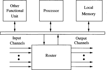

Figure 1.5 Strictly orthogonal direct network topologies: (a) 2-ary 4-cube (hypercube), (b) 3-ary 2-cube, and (c) 3-ary 3-D mesh.
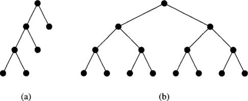
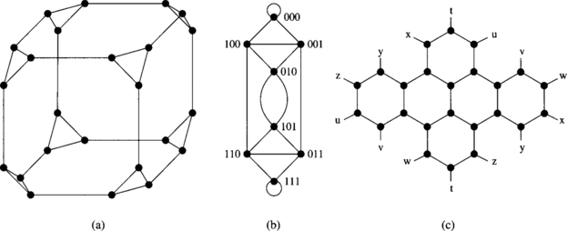
Figure 1.7 Other direct network topologies: (a) cube-connected cycles, (b) de Bruijn network, and (c) star graph.
Each router supports some number of input and output channels. Internal channels or ports connect the local processor/memory to the router. Although it is common to provide only one pair of internal channels, some systems use more internal channels in order to avoid a communication bottleneck between the local processor/memory and the router [39]. External channels are used for communication between routers. By connecting input channels of one node to the output channels of other nodes, the direct network is defined. Unless otherwise specified, the term “channel” will refer to an external channel. Two directly connected nodes are called neighboring or adjacent nodes. Usually, each node has a fixed number of input and output channels, and every input channel is paired with a corresponding output channel. Through the connections among these channels, there are many ways to interconnect these nodes. Obviously, every node in the network should be able to reach every other node.
1.6.1 Characterization of Direct Networks
Direct networks have been traditionally modeled by a graph G(N, C), where the vertices of the graph N represent the set of processing nodes and the edges of the graph C represent the set of communication channels. This is a very simple model that does not consider implementation issues. However, it allows the study of many interesting network properties. Depending on the properties under study, a bidirectional channel may be modeled either as an edge or as two arcs in opposite directions (two unidirectional channels). The latter is the case for deadlock avoidance in Chapter 3. Let us assume that a bidirectional channel is modeled as an edge. Some basic network properties can be defined from the graph representation:
![]() Node degree: Number of channels connecting that node to its neighbors.
Node degree: Number of channels connecting that node to its neighbors.
![]() Diameter: The maximum distance between two nodes in the network.
Diameter: The maximum distance between two nodes in the network.
![]() Regularity: A network is regular when all the nodes have the same degree.
Regularity: A network is regular when all the nodes have the same degree.
![]() Symmetry: A network is symmetric when it looks alike from every node.
Symmetry: A network is symmetric when it looks alike from every node.
A direct network is mainly characterized by three factors: topology, routing, and switching. The topology defines how the nodes are interconnected by channels and is usually modeled by a graph as indicated above. For direct networks, the ideal topology would connect every node to every other node. No message would even have to pass through an intermediate node before reaching its destination. This fully connected topology requires a router with N links (including the internal one) at each node for a network with N nodes. Therefore, the cost is prohibitive for networks of moderate to large size. Additionally, the number of physical connections of a node is limited by hardware constraints such as the number of available pins and the available wiring area. These engineering and scaling difficulties preclude the use of such fully connected networks even for small network sizes. As a consequence, many topologies have been proposed, trying to balance performance and some cost parameters. In these topologies, messages may have to traverse some intermediate nodes before reaching the destination node.
From the programmer’s perspective, the unit of information exchange is the message. The size of messages may vary depending on the application. For efficient and fair use of network resources, a message is often divided into packets prior to transmission. A packet is the smallest unit of communication that contains the destination address and sequencing information, which are carried in the packet header. For topologies in which packets may have to traverse some intermediate nodes, the routing algorithm determines the path selected by a packet to reach its destination. At each intermediate node, the routing algorithm indicates the next channel to be used. That channel may be selected among a set of possible choices. If all the candidate channels are busy, the packet is blocked and cannot advance. Obviously, efficient routing is critical to the performance of interconnection networks.
When a message or packet header reaches an intermediate node, a switching mechanism determines how and when the router switch is set; that is, the input channel is connected to the output channel selected by the routing algorithm. In other words, the switching mechanism determines how network resources are allocated for message transmission. For example, in circuit switching, all the channels required by a message are reserved before starting message transmission. In packet switching, however, a packet is transmitted through a channel as soon as that channel is reserved, but the next channel is not reserved (assuming that it is available) until the packet releases the channel it is currently using. Obviously, some buffer space is required to store the packet until the next channel is reserved. That buffer should be allocated before starting packet transmission. So, buffer allocation is closely related to the switching mechanism. Flow control is also closely related to the switching and buffer allocation mechanisms. The flow control mechanism establishes a dialog between sender and receiver nodes, allowing and stopping the advance of information. If a packet is blocked, it requires some buffer space to be stored. When there is no more available buffer space, the flow control mechanism stops information transmission. When the packet advances and buffer space is available, transmission is started again. If there is no flow control and no more buffer space is available, the packet may be dropped or derouted through another channel.
The above factors affect the network performance. They are not independent of each other but are closely related. For example, if a switching mechanism reserves resources in an aggressive way (as soon as a packet header is received), packet latency can be reduced. However, each packet may be holding several channels at the same time. So, such a switching mechanism may cause severe network congestion and, consequently, make the design of efficient routing and flow control policies difficult. The network topology also affects performance, as well as how the network traffic can be distributed over available channels. In most cases, the choice of a suitable network topology is restricted by wiring and packaging constraints.
1.6.2 Popular Network Topologies
Many network topologies have been proposed in terms of their graph-theoretical properties. However, very few of them have ever been implemented. Most of the implemented networks have an orthogonal topology. A network topology is orthogonal if and only if nodes can be arranged in an orthogonal n-dimensional space, and every link can be arranged in such a way that it produces a displacement in a single dimension. Orthogonal topologies can be further classified as strictly orthogonal and weakly orthogonal. In a strictly orthogonal topology, every node has at least one link crossing each dimension. In a weakly orthogonal topology, some nodes may not have any link in some dimensions.
Hence, it is not possible to cross every dimension from every node. Crossing a given dimension from a given node may require moving in another dimension first.
Strictly Orthogonal Topologies
The most interesting property of strictly orthogonal topologies is that routing is very simple. Thus, the routing algorithm can be efficiently implemented in hardware. Effectively, in a strictly orthogonal topology, nodes can be numbered by using their coordinates in the n-dimensional space. Since each link traverses a single dimension and every node has at least one link crossing each dimension, the distance between two nodes can be computed as the sum of dimension offsets. Also, the displacement along a given link only modifies the offset in the corresponding dimension. Taking into account that it is possible to cross any dimension from any node in the network, routing can be easily implemented by selecting a link that decrements the absolute value of the offset in some dimension. The set of dimension offsets can be stored in the packet header and updated (by adding or subtracting one unit) every time the packet is successfully routed at some intermediate node. If the topology is not strictly orthogonal, however, routing may become much more complex.
The most popular direct networks are the n-dimensional mesh, the k-ary n-cube or torus, and the hypercube. All of them are strictly orthogonal. Formally, an n-dimensional mesh has k0 × k1 × … × kn−2 × kn−1 nodes, ki nodes along each dimension i, where ki ≥ 2 and 0 ≤ i ≤ n − 1. Each node X is identified by n coordinates, (xn−1, xn−2, …, x1, x0), where 0 ≤ xi ≤ ki − 1 for 0 ≤ i ≤ n − 1. Two nodes X and Y are neighbors if and only if yi = xi for all i, 0 ≤ i ≤ n − 1, except one, j, where yj = xj ± 1. Thus, nodes have from n to 2n neighbors, depending on their location in the mesh. Therefore, this topology is not regular.
In a bidirectional k-ary n-cube [70], all nodes have the same number of neighbors. The definition of a k-ary n-cube differs from that of an n-dimensional mesh in that all of the ki are equal to k and two nodes X and Y are neighbors if and only if yi = xi for all i, 0 ≤i≤ n − 1, except one, j, where yj = (xj ± 1) mod k. The change to modular arithmetic in the definition adds wraparound channels to the k-ary n-cube, giving it regularity and symmetry. Every node has n neighbors if k = 2, and 2n neighbors if k > 2. When n = 1, the k-ary n-cube collapses to a bidirectional ring with k nodes.
Another topology with regularity and symmetry is the hypercube, which is a special case of both n-dimensional meshes and k-ary n-cubes. A hypercube is an n-dimensional mesh in which ki = 2 for 0 ≤ i ≤ n − 1, or a 2-ary n-cube, also referred to as a binary n-cube.
Figure 1.5(a) depicts a binary 4-cube or 16-node hypercube. Figure 1.5(b) illustrates a 3-ary 2-cube or two-dimensional (2-D) torus. Figure 1.5(c) shows a 3-ary three-dimensional (3-D) mesh, resulting by removing the wraparound channels from a 3-ary 3-cube.
Two conflicting requirements of a direct network are that it must accommodate a large number of nodes while maintaining a low network latency. This issue will be addressed in Chapter 7.
Other Direct Network Topologies
A popular topology is the tree. This topology has a root node connected to a certain number of descendant nodes. Each of these nodes is in turn connected to a disjoint set (possibly empty) of descendants. A node with no descendants is a leaf node. A characteristic property of trees is that every node but the root has a single parent node. Therefore, trees contain no cycles. A tree in which every node but the leaves has a fixed number k of descendants is a k-ary tree. When the distance from every leaf node to the root is the same (i.e., all the branches of the tree have the same length), the tree is balanced. Figure 1.6(a) and (b) shows an unbalanced and a balanced binary tree, respectively.
The most important drawback of trees as general-purpose interconnection networks is that the root node and the nodes close to it become a bottleneck. Additionally, there are no alternative paths between any pair of nodes. The bottleneck can be removed by allocating a higher channel bandwidth to channels located close to the root node. The shorter the distance to the root node, the higher the channel bandwidth. However, using channels with different bandwidths is not practical, especially when message transmission is pipelined. A practical way to implement trees with higher channel bandwidth in the vicinity of the root node (fat trees) will be described in Section 1.7.5.
One of the most interesting properties of trees is that, for any connected graph, it is possible to define a tree that spans the complete graph. As a consequence, for any connected network, it is possible to build an acyclic network connecting all the nodes by removing some links. This property can be used to define a routing algorithm for any irregular topology. However, that routing algorithm may be inefficient due to the concentration of traffic across the root node. A possible way to circumvent that limitation will be presented in Section 4.9.
Some topologies have been proposed with the purpose of reducing node degree while keeping the diameter small. Most of these topologies can be viewed as a hierarchy of topologies. This is the case for the cube-connected cycles [284] This topology can be considered as an n-dimensional hypercube of virtual nodes, where each virtual node is a ring with n nodes, for a total of n2n nodes. Each node in the ring is connected to a single dimension of the hypercube. Therefore, node degree is fixed and equal to three: two links connecting to neighbors in the ring, and one link connecting to a node in another ring through one of the dimensions of the hypercube. However, the diameter is of the same order of magnitude as that of a hypercube of similar size. Figure 1.7(a) shows a 24-node cube-connected cycles network. It is worth noting that cube-connected cycles are weakly orthogonal because the ring is a one-dimensional network, and displacement inside the ring does not change the position in the other dimensions. Similarly, a displacement along a hypercube dimension does not affect the position in the ring. However, it is not possible to cross every dimension from each node.
Many topologies have been proposed with the purpose of minimizing the network diameter for a given number of nodes and node degree. Two well-known topologies proposed with this purpose are the de Bruijn network and the star graphs. In the de Bruijn network [301] there are dn nodes, and each node is represented by a set of n digits in base d. A node (xn−1, xn−2, …, x1, x0), where 0 ≤ xi ≤ d − 1 for 0 ≤ i ≤ n − 1, is connected to nodes (xn−2, …, x1, x0, p) and (p, xn−1, xn−2, …, x1), for all p such that 0 ≤ p ≤ d − 1. In other words, two nodes are connected if the representation of one node is a right or left shift of the representation of the other. Figure 1.7(b) shows an eight-node de Bruijn network. When networks are very large, this network topology achieves a very low diameter for a given number of nodes and node degree. However, routing is complex. Additionally, the average distance between nodes is high, close to the network diameter. Finally, some nodes have links connecting to themselves. All of these issues make the practical application of these networks very difficult.
A star graph [6] can be informally described as follows. The vertices of the graph are labeled by permutations of n different symbols, usually denoted as 1 to n. A permutation is connected to every other permutation that can be obtained from it by interchanging the first symbol with any of the other symbols. A star graph has n! nodes, and node degree is equal to n − 1. Figure 1.7(c) shows a star graph obtained by permutations of four symbols. Although a star graph has a lower diameter than a hypercube of similar size, routing is more complex. Star graphs were proposed as a particular case of Cayley graphs [6]. Other topologies like hypercubes and cube-connected cycles are also particular cases of Cayley graphs.
1.6.3 Examples
Several examples of parallel computers with direct networks and the main characteristics are listed below.
![]() Cray T3E: Bidirectional 3-D torus, 14-bit data in each direction, 375 MHz link speed, 600 Mbytes/s per link.
Cray T3E: Bidirectional 3-D torus, 14-bit data in each direction, 375 MHz link speed, 600 Mbytes/s per link.
![]() Cray T3D: Bidirectional 3-D torus, up to 1,024 nodes (8 × 16 × 8), 24-bit links (16-bit data, 8-bit control), 150 MHz, 300 Mbytes/s per link.
Cray T3D: Bidirectional 3-D torus, up to 1,024 nodes (8 × 16 × 8), 24-bit links (16-bit data, 8-bit control), 150 MHz, 300 Mbytes/s per link.
![]() Intel Cavallino: Bidirectional 3-D topology, 16-bit-wide channels operating at 200 MHz, 400 Mbytes/s in each direction.
Intel Cavallino: Bidirectional 3-D topology, 16-bit-wide channels operating at 200 MHz, 400 Mbytes/s in each direction.
![]() SGI SPIDER: Router with 20-bit bidirectional channels operating on both edges, 200 MHz clock, aggregate raw data rate of 1 Gbyte/s. Support for regular and irregular topologies.
SGI SPIDER: Router with 20-bit bidirectional channels operating on both edges, 200 MHz clock, aggregate raw data rate of 1 Gbyte/s. Support for regular and irregular topologies.
![]() MIT M-Machine: 3-D mesh, 800 Mbytes/s for each network channel.
MIT M-Machine: 3-D mesh, 800 Mbytes/s for each network channel.
![]() MIT Reliable Router: 2-D mesh, 23-bit links (16-bit data), 200 MHz, 400 Mbytes/s per link per direction, bidirectional signaling, reliable transmission.
MIT Reliable Router: 2-D mesh, 23-bit links (16-bit data), 200 MHz, 400 Mbytes/s per link per direction, bidirectional signaling, reliable transmission.
![]() Chaos Router: 2-D torus topology, bidirectional 8-bit links, 180 MHz, 360 Mbytes/s in each direction.
Chaos Router: 2-D torus topology, bidirectional 8-bit links, 180 MHz, 360 Mbytes/s in each direction.
![]() Intel iPSC-2 Hypercube: Binary hypercube topology, bit-serial channels at 2.8 Mbytes/s.
Intel iPSC-2 Hypercube: Binary hypercube topology, bit-serial channels at 2.8 Mbytes/s.
1.7 Indirect Networks
Indirect or switch-based networks are another major class of interconnection networks. Instead of providing a direct connection among some nodes, the communication between any two nodes has to be carried through some switches. Each node has a network adapter that connects to a network switch. Each switch can have a set of ports. Each port consists of one input and one output link. A (possibly empty) set of ports in each switch is either connected to processors or left open, whereas the remaining ports are connected to ports of other switches to provide connectivity between the processors. The interconnection of those switches defines various network topologies.
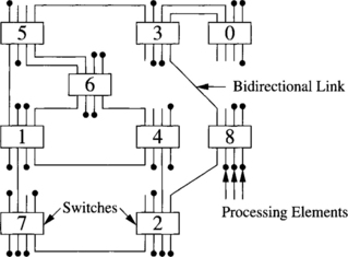
Switch-based networks have evolved considerably over time. A wide range of topologies has been proposed, ranging from regular topologies used in array processors and shared-memory UMA multiprocessors to the irregular topologies currently used in NOWs. Both network classes will be covered in this book. Regular topologies have regular connection patterns between switches, while irregular topologies do not follow any predefined pattern. Figures 1.19 and 1.21 show several switch-based networks with regular topology. The corresponding connection patterns will be studied later. Figure 1.8 shows a typical switch-based network with irregular topology. Both network classes can be further classified according to the number of switches a message has to traverse before reaching its destination. Although this classification is not important in the case of irregular topologies, it makes a big difference in the case of regular networks because some specific properties can be derived for each network class.
1.7.1 Characterization of Indirect Networks
Indirect networks can also be modeled by a graph G(N, C), where N is the set of switches and C is the set of unidirectional or bidirectional links between the switches. For the analysis of most properties, it is not necessary to explicitly include processing nodes in the graph. Although a similar model can be used for direct and indirect networks, a few differences exist between them. Each switch in an indirect network may be connected to zero, one, or more processors. Obviously, only the switches connected to some processor can be the source or the destination of a message. Additionally, transmitting a message from a node to another node requires crossing the link between the source node and the switch connected to it, and the link between the last switch in the path and the destination node. Therefore, the distance between two nodes is the distance between the switches directly connected to those nodes plus two units. Similarly, the diameter is the maximum distance between two switches connected to some node plus two units. It may be argued that it is not necessary to add two units because direct networks also have internal links between routers and processing nodes. However, those links are external in the case of indirect networks. This gives a consistent view of the diameter as the maximum number of external links between two processing nodes. In particular, the distance between two nodes connected through a single switch is two instead of zero.
Similar to direct networks, an indirect network is mainly characterized by three factors: topology, routing, and switching. The topology defines how the switches are interconnected by channels and can be modeled by a graph as indicated above. For indirect networks with N nodes, the ideal topology would connect those nodes through a single N × N switch. Such a switch is known as a crossbar. Although using a single N × N crossbar is much cheaper than using a fully connected direct network topology (requiring N routers, each one having an internal N × N crossbar), the cost is still prohibitive for large networks. Similar to direct networks, the number of physical connections of a switch is limited by hardware constraints such as the number of available pins and the available wiring area. These engineering and scaling difficulties preclude the use of crossbar networks for large network sizes. As a consequence, many alternative topologies have been proposed. In these topologies, messages may have to traverse several switches before reaching the destination node. In regular networks, these switches are usually identical and have been traditionally organized as a set of stages. Each stage (but the input/output stages) is only connected to the previous and next stages using regular connection patterns. Input/output stages are connected to the nodes as well as to another stage in the network. These networks are referred to as multistage interconnection networks and have different properties depending on the number of stages and how those stages are arranged.
The remaining issues discussed in Section 1.6.1 (routing, switching, flow control, buffer allocation, and their impact on performance) are also applicable to indirect networks.
1.7.2 Crossbar Networks
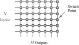
Crossbar networks allow any processor in the system to connect to any other processor or memory unit so that many processors can communicate simultaneously without contention. A new connection can be established at any time as long as the requested input and output ports are free. Crossbar networks are used in the design of high-performance small-scale multiprocessors, in the design of routers for direct networks, and as basic components in the design of large-scale indirect networks. A crossbar can be defined as a switching network with N inputs and M outputs, which allows up to min{N, M} one-to-one interconnections without contention. Figure 1.9 shows an N × M crossbar network. Usually, M = N except for crossbars connecting processors and memory modules.
The cost of such a network is O(N M), which is prohibitively high with large N and M. Crossbar networks have been traditionally used in small-scale shared-memory multiprocessors, where all processors are allowed to access memories simultaneously as long as each processor reads from, or writes to, a different memory. When two or more processors contend for the same memory module, arbitration lets one processor proceed while the others wait. The arbiter in a crossbar is distributed among all the switch points connected to the same output. However, the arbitration scheme can be less complex than the one for a bus because conflicts in crossbar are the exception rather than the rule, and therefore easier to resolve.
For a crossbar network with distributed control, each switch point may have four states, as shown in Figure 1.10. In Figure 1.10(a), the input from the row containing the switch point has been granted access to the corresponding output, while inputs from upper rows requesting the same output are blocked. In Figure 1.10(b), an input from an upper row has been granted access to the output. The input from the row containing the switch point does not request that output and can be propagated to other switches. In Figure 1.10(c), an input from an upper row has also been granted access to the output. However, the input from the row containing the switch point also requests that output and is blocked. The configuration in Figure 1.10(d) is only required if the crossbar has to support multicasting (one-to-many communication).
The advent of VLSI permitted the integration of hardware for thousands of switches into a single chip. However, the number of pins on a VLSI chip cannot exceed a few hundred, which restricts the size of the largest crossbar that can be integrated into a single VLSI chip. Large crossbars can be realized by partitioning them into smaller crossbars, each one implemented using a single chip. Thus, a full crossbar of size N × N can be implemented with (N/n)(N/n)n × n crossbars.
1.7.3 Multistage Interconnection Networks
Multistage interconnection networks (MINs) connect input devices to output devices through a number of switch stages, where each switch is a crossbar network. The number of stages and the connection patterns between stages determine the routing capability of the networks.
MINs were initially proposed for telephone networks and later for array processors. In these cases, a central controller establishes the path from input to output. In cases where the number of inputs equals the number of outputs, each input synchronously transmits a message to one output, and each output receives a message from exactly one input. Such unicast communication patterns can be represented as a permutation of the input addresses. For this application, MINs have been popular as alignment networks for storing and accessing arrays in parallel from memory banks. Array storage is typically skewed to permit conflict-free access, and the network is used to unscramble the arrays during access. These networks can also be configured with the number of inputs greater than the number of outputs (concentrators) and vice versa (expanders). On the other hand, in asynchronous multiprocessors, centralized control and permutation routing are infeasible. In this case, a routing algorithm is required to establish the path across the stages of a MIN.
Depending on the interconnection scheme employed between two adjacent stages and the number of stages, various MINs have been proposed. MINs are good for constructing parallel computers with hundreds of processors and have been used in some commercial machines.
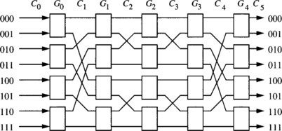
1.7.4 A Generalized MIN Model
There are many ways to interconnect adjacent stages. Figure 1.11 shows a generalized multistage interconnection network with N inputs and M outputs. It has g stages, G0 to Gg−1. As shown in Figure 1.12, each stage, say, Gi, has wi switches of size ai, j × bi, j, where 1 ≤ j ≤ wi. Thus, stage Gi has pi inputs and qi outputs, where
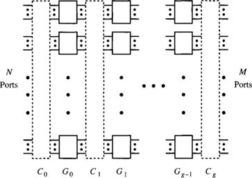
The connection between two adjacent stages, Gi−1 and Gi, denoted Ci, defines the connection pattern for pi = qi−1 links, where p0 = N and qg−1 = M. A MIN thus can be represented as
A connection pattern Ci (pi) defines how those pi links should be connected between the qi−1 = pi outputs from stage Gi−1 and the pi inputs to stage Gi. Different connection patterns give different characteristics and topological properties of MINs. The links are labeled from 0 to pi − 1 at Ci.
In practice, all the switches will be identical, thus amortizing the design cost. Banyan networks are a class of MINs with the property that there is a unique path between any pair of source and destination [132]. An N-node (N = kn) Delta network is a subclass of banyan networks, which is constructed from identical k × k switches in n stages, where each stage contains ![]() switches. Many of the known MINs, such as Omega, flip, cube, butterfly, and baseline, belong to the class of Delta networks [273] and have been shown to be topologically and functionally equivalent [352]. A good survey of those MINs can be found in [318]. Some of those MINs are defined below.
switches. Many of the known MINs, such as Omega, flip, cube, butterfly, and baseline, belong to the class of Delta networks [273] and have been shown to be topologically and functionally equivalent [352]. A good survey of those MINs can be found in [318]. Some of those MINs are defined below.
When switches have the same number of input and output ports, MINs also have the same number of input and output ports. Since there is a one-to-one correspondence between inputs and outputs, the connections between stages are also called permutations. Five basic permutations are defined below. Although these permutations were originally defined for networks with 2 × 2 switches, for most definitions we assume that the network is built by using k × k switches, and that there are N = kn inputs and outputs, where n is an integer. However, some of these permutations are only defined for the case where N is a power of 2. With N = kn ports, let X = xn−1 xn−2… x0 be an arbitrary port number, 0 ≤ X ≤ N − 1, where 0 ≤ xi ≤ k − 1, 0 ≤ i ≤ n − 1.
Perfect Shuffle Permutation
The perfect k-shuffle permutation σk is defined by
A more cogent way to describe the perfect k-shuffle permutation σk is
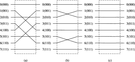
The perfect k-shuffle permutation performs a cyclic shifting of the digits in X to the left for one position. For k = 2, this action corresponds to perfectly shuffling a deck of N cards, as demonstrated in Figure 1.13(a) for the case of N = 8. The perfect shuffle cuts the deck into two halves from the center and intermixes them evenly. The inverse perfect shuffle permutation does the opposite, as defined by
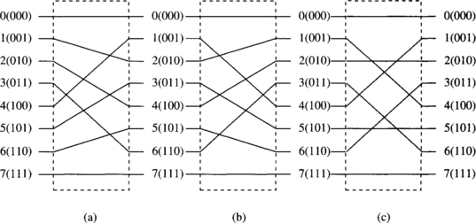
Figure 1.13 (a) The perfect shuffle, (b) inverse perfect shuffle, and (c) bit reversal permutations for N = 8.
Figure 1.13(b) demonstrates an inverse perfect shuffle permutation.
Digit Reversal Permutation
The digit reversal permutation ρk is defined by
This permutation is usually referred to as bit reversal, clearly indicating that it was proposed for k = 2. However, its definition is also valid for k > 2. Figure 1.13(c) demonstrates a bit reversal permutation for the case of k = 2 and N = 8.
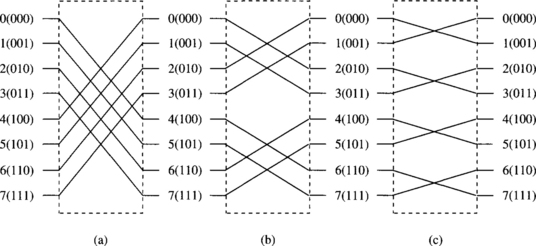
Butterfly Permutation
The ith k-ary butterfly permutation ![]() , for 0 ≤ i ≤ n − 1, is defined by
, for 0 ≤ i ≤ n − 1, is defined by
The ith butterfly permutation interchanges the zeroth and ith digits of the index. Figure 1.14 shows the butterfly permutation for k = 2, and i= 0, 1, and 2 with N = 8. Note that ![]() defines a straight one-to-one permutation and is also called identity permutation, I.
defines a straight one-to-one permutation and is also called identity permutation, I.
Cube Permutation
The ith cube permutation Ei, for 0 ≤ i ≤ n − 1, is defined only for k = 2 by
The ith cube permutation complements the ith bit of the index. Figure 1.15 shows the cube permutation for i = 0, 1, and 2 with N = 8. E0 is also called the exchange permutation.
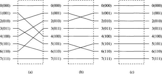
Baseline Permutation
The ith k-ary baseline permutation ![]() , for 0 ≤ i ≤ n − 1, is defined by
, for 0 ≤ i ≤ n − 1, is defined by
The ith baseline permutation performs a cyclic shifting of thei+ 1 least significant digits in the index to the right for one position. Figure 1.16 shows the baseline permutation for k = 2, andi= 0, 1, and 2 with N = 8. Note that ![]() also defines the identity permutation I.
also defines the identity permutation I.
1.7.5 Classification of Multistage Interconnection Networks
Depending on the availability of paths to establish new connections, MINs have been traditionally divided into three classes:
1. Blocking. A connection between a free input/output pair is not always possible because of conflicts with the existing connections. Typically, there is a unique path between every input/output pair, thus minimizing the number of switches and stages. However, it is also possible to provide multiple paths to reduce conflicts and increase fault tolerance. These blocking networks are also known as multipath networks.
2. Nonblocking. Any input port can be connected to any free output port without affecting the existing connections. Nonblocking networks have the same functionality as a crossbar. They require multiple paths between every input and output, which in turn leads to extra stages.
3. Rearrangeable. Any input port can be connected to any free output port. However, the existing connections may require rearrangement of paths. These networks also require multiple paths between every input and output, but the number of paths and the cost is smaller than in the case of nonblocking networks.
Nonblocking networks are expensive. Although they are cheaper than a crossbar of the same size, their cost is prohibitive for large sizes. The best-known example of a nonblocking multistage network is the Clos network, initially proposed for telephone networks. Rearrangeable networks require less stages or simpler switches than a nonblocking network. The best-known example of a rearrangeable network is the Beneš network. Figure 1.17 shows an 8 × 8 Beneš network. For 2n inputs, this network requires 2n − 1 stages and provides 2n −1 alternative paths. Rearrangeable networks require a central controller to rearrange connections and were proposed for array processors. However, connections cannot be easily rearranged on multiprocessors because processors access the network asynchronously. So, rearrangeable networks behave like blocking networks when accesses are asynchronous. Thus, this class has not been included in Figure 1.2. We will mainly focus on blocking networks.
Depending on the kind of channels and switches, MINs can be split into two classes [254]:
1. Unidirectional MINs. Channels and switches are unidirectional.
2. Bidirectional MINs. Channels and switches are bidirectional. This implies that information can be transmitted simultaneously in opposite directions between neighboring switches.
Additionally, each channel may be either multiplexed or replaced by two or more channels. In the latter case, the network is referred to as dilated MIN. Obviously, the number of ports of each switch must increase accordingly.
Unidirectional Multistage Interconnection Networks
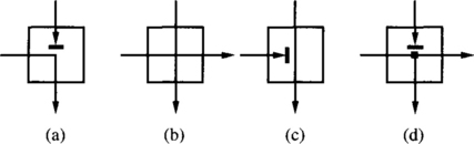
The basic building blocks of unidirectional MINs are unidirectional switches. An a × b switch is a crossbar network with a inputs and b outputs. If each input port is allowed to connect to exactly one output port, at most min {a, b} connections can be supported simultaneously. If each input port is allowed to connect to many output ports, a more complicated design is needed to support the so-called one-to-many or multicast communication. In the broadcast mode or one-to-all communication, each input port is allowed to connect to all output ports. Figure 1.18 shows four possible states of a 2 × 2 switch. The last two states are used to support one-to-many and one-to-all communications.
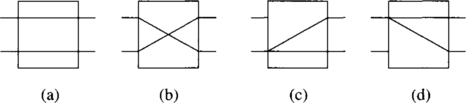
Figure 1.18 Four possible states of a 2 × 2 switch: (a) straight, (b) exchange, (c) lower broadcast, and (d) upper broadcast.
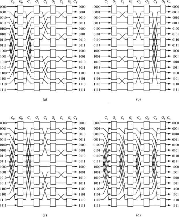
Figure 1.19 Four 16 × 16 unidirectional multistage interconnection networks: (a) baseline network, (b) butterfly network, (c) cube network, and (d) Omega network.
In MINs with N = M, it is common to use switches with the same number of input and output ports, that is, a = b. If N > M, switches with a > b will be used. Such switches are also called concentration switches. In the case of N < M, distribution switches with a < b will be used.
It can be shown that with N input and output ports, a unidirectional MIN with k × k switches requires at least [logk N] stages to allow a connection path between any input port and any output port. By having additional stages, more connection paths may be used to deliver a message between an input port and an output port at the expense of extra hardware cost. Every path through the MIN crosses all the stages. Therefore, all the paths have the same length.
Four topologically equivalent unidirectional MINs are considered below. These MINs are a class of Delta networks.
1. Baseline MINs. In a baseline MIN, connection pattern Ci is described by the (n − i)th baseline permutation ![]() for 1 ≤ i ≤ n. Connection pattern C0 is selected to be σk.
for 1 ≤ i ≤ n. Connection pattern C0 is selected to be σk.
2. Butterfly MINs. In a butterfly MIN, connection pattern Ci is described by the ith butterfly permutation ![]() for 0 ≤ i ≤ n − 1. Connection pattern Cn is selected to be
for 0 ≤ i ≤ n − 1. Connection pattern Cn is selected to be ![]() .
.
3. Cube MINs. In a cube MIN (or multistage cube network [318]), connection pattern Ci is described by the (n − i)th butterfly permutation ![]() for 1 ≤ i ≤ n. Connection pattern C0 is selected to be σk.
for 1 ≤ i ≤ n. Connection pattern C0 is selected to be σk.
4. Omega network. In an Omega network, connection pattern Ci is described by the perfect k-shuffle permutation σk for 0 ≤ i ≤ n − 1. Connection pattern Cn is selected to be ![]() . Thus, all the connection patterns but the last one are identical. The last connection pattern produces no permutation.
. Thus, all the connection patterns but the last one are identical. The last connection pattern produces no permutation.
The topological equivalence of these MINs can be viewed as follows: Consider that each input link to the first stage is numbered using a string of n digits sn−1sn−2 …s1s0, where 0 ≤ si ≤ k − 1, for 0 ≤ i ≤ n − 1. The least significant digit s0 gives the address of the input port at the corresponding switch, and the address of the switch is given by sn−1sn−2 …s1. At each stage, a given switch is able to connect any input port with any output port. This can be viewed as changing the value of the least significant digit of the address. In order to be able to connect any input to any output of the network, it should be possible to change the value of all the digits. As each switch is only able to change the value of the least significant digit of the address, connection patterns between stages are defined in such a way that the position of digits is permuted, and after n stages all the digits have occupied the least significant position. Therefore, the above-defined MINs differ in the order in which address digits occupy the least significant position.
Figure 1.19 shows the topology of four 16 × 16 unidirectional multistage interconnection networks: (a) baseline network, (b) butterfly network, (c) cube network, and (d) Omega network.
Bidirectional Multistage Interconnection Networks
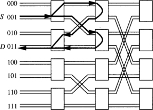
Figure 1.20 illustrates a bidirectional switch in which each port is associated with a pair of unidirectional channels in opposite directions. This implies that information can be transmitted simultaneously in opposite directions between neighboring switches. For ease of explanation, it is assumed that processor nodes are on the left-hand side of the network, as shown in Figure 1.21. A bidirectional switch supports three types of connections: forward, backward, and turnaround (see Figure 1.20). As turnaround connections between ports at the same side of a switch are possible, paths have different lengths. An eight-node butterfly bidirectional MIN (BMIN) is illustrated in Figure 1.21.
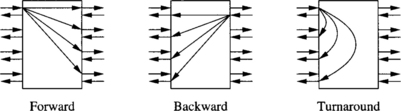
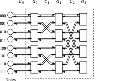
Paths are established in BMINs by crossing stages in the forward direction, then establishing a turnaround connection, and finally crossing stages in the backward direction. This is usually referred to as turnaround routing. Figure 1.22 shows two alternative paths from node S to node D in an eight-node butterfly BMIN. When crossing stages in the forward direction, several paths are possible. Each switch can select any of its output ports. However, once the turnaround connection is crossed, a single path is available up to the destination node. In the worst case, establishing a path in an n-stage BMIN requires crossing 2n − 1 stages. This behavior closely resembles that of the Beneš network. Indeed, the baseline BMIN can be considered as a folded Beneš network.
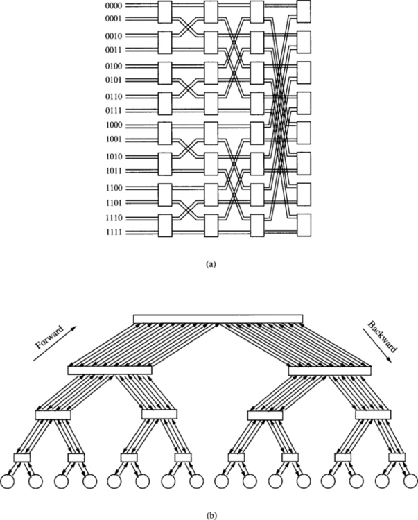
As shown in Figure 1.23, a butterfly BMIN with turnaround routing can be viewed as a fat tree [201]. In a fat tree, processors are located at leaves, and internal vertices are switches. Transmission bandwidth between switches is increased by adding more links in parallel as switches become closer to the root switch. When a message is routed from one processor to another, it is sent up (in the forward direction) the tree to the least common ancestor of the two processors, and then sent down (in the backward direction) to the destination. Such a tree routing well explains the turnaround routing mentioned above.
1.7.6 Examples
Several examples of parallel computers with indirect networks and commercial switches to build indirect networks are listed below:
![]() Myricom Myrinet: Supports regular and irregular topologies, 8 × 8 crossbar switch, 9-bit channels, full-duplex, 160 Mbytes/s per link.
Myricom Myrinet: Supports regular and irregular topologies, 8 × 8 crossbar switch, 9-bit channels, full-duplex, 160 Mbytes/s per link.
![]() Thinking Machines CM-5: Fat tree topology, 4-bit bidirectional channels at 40 MHz, aggregate bandwidth in each direction of 20 Mbytes/s.
Thinking Machines CM-5: Fat tree topology, 4-bit bidirectional channels at 40 MHz, aggregate bandwidth in each direction of 20 Mbytes/s.
![]() Inmos C104: Supports regular and irregular topologies, 32 × 32 crossbar switch, serial links, 100 Mbits/s per link.
Inmos C104: Supports regular and irregular topologies, 32 × 32 crossbar switch, serial links, 100 Mbits/s per link.
![]() IBM SP2: Crossbar switches supporting Omega network topologies with bidirectional, 16-bit channels at 150MHz, 300 Mbytes/s in each direction.
IBM SP2: Crossbar switches supporting Omega network topologies with bidirectional, 16-bit channels at 150MHz, 300 Mbytes/s in each direction.
![]() SGI SPIDER: Router with 20-bit bidirectional channels operating on both edges, 200 MHz clock, aggregate raw data rate of 1 Gbyte/s. Offers support for configurations as nonblocking multistage network topologies as well as irregular topologies.
SGI SPIDER: Router with 20-bit bidirectional channels operating on both edges, 200 MHz clock, aggregate raw data rate of 1 Gbyte/s. Offers support for configurations as nonblocking multistage network topologies as well as irregular topologies.
![]() Tandem ServerNet: Irregular topologies, 8-bit bidirectional channels at 50 MHz, 50 Mbytes/s per link.
Tandem ServerNet: Irregular topologies, 8-bit bidirectional channels at 50 MHz, 50 Mbytes/s per link.
1.8 Hybrid Networks
In this section, we briefly describe some network topologies that do not fit into the classes described above. In general, hybrid networks combine mechanisms from shared-medium networks and direct or indirect networks. Therefore, they increase bandwidth with respect to shared-medium networks and reduce the distance between nodes with respect to direct and indirect networks. There exist well-established applications of hybrid networks. This is the case for bridged LANs. However, for systems requiring very high performance, direct and indirect networks achieve better scalability than hybrid networks because point-to-point links are simpler and faster than shared-medium buses. Most high-performance parallel computers use direct or indirect networks. Recently, hybrid networks have been gaining acceptance again. The use of optical technology enables the implementation of high-performance buses. Currently, some prototype machines are being implemented based on electrical as well as optical interconnects.
Many hybrid networks have been proposed for different purposes. The classification proposed for these networks is mainly dictated by the application fields. In general, hybrid networks can be modeled by a hypergraph [23], where the vertices of the hypergraph represent the set of processing nodes and the edges represent the set of communication channels and/or buses. Note that an edge in a hypergraph can interconnect an arbitrary number of nodes. When an edge connects exactly two nodes, then it represents a point-to-point channel. Otherwise it represents a bus. In some network designs, each bus has a single driving node. No other device is allowed to drive that bus. In this case, there is no need for arbitration. However, it is still possible to have several receivers at a given time, thus retaining the broadcast capability of buses. Obviously, every node in the network must drive at least one bus, therefore requiring a number of buses not lower than the number of nodes. In this case, the network topology can be modeled by a directed hypergraph.
1.8.1 Multiple Backplane Buses
Due to limited shared-medium network bandwidth, a shared-medium network can only support a small number of devices, has limited distance, and is not scalable to support a large system. Some approaches have been used or studied to remove such bottlenecks. One approach to increase network bandwidth is to have multiple buses as shown in Figure 1.24. However, concern about wiring and interface costs is a major reason why multiple buses have seen little use so far in multiprocessor design [246]. Due to the limitations of electrical packaging technology, it is unlikely to have a multiple-bus network with more than four buses. However, many more buses are likely feasible with other packaging technologies such as wavelength division multiplexing on fiber optics [280].
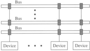
1.8.2 Hierarchical Networks
Another approach to increase the network bandwidth is to have a hierarchical structure as shown in Figure 1.25. Different buses are interconnected by routers or bridges to transfer information from one side of the network to the other side of the network. These routers or bridges can filter the network traffic by examining the destination address of each passing message. The hierarchical network can expand the network area and handle more devices, but it is no longer a simple shared-medium network. This approach is used in bridged LANs. Usually, a higher bandwidth is available at the global bus. Otherwise, it may become a bottleneck. This can be achieved by using a faster technology. This is the case for the backbone LAN in some bridged LANs. Hierarchical networks have also been proposed as the interconnection scheme for shared-memory multiprocessors. Again, the global bus may become a bottleneck. For example, the Encore Gigamax addressed this problem by having an optical fiber bus to increase the bandwidth of the global bus.
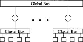
1.8.3 Cluster-Based Networks
Cluster-based networks also have a hierarchical structure. Indeed, they can be considered as a subclass of hierarchical networks. Cluster-based networks combine the advantages of two or more kinds of networks at different levels in the hierarchy. For example, it is possible to combine the advantages of buses and point-to-point links by using buses at the lower level in the hierarchy to form clusters and a direct network topology connecting clusters at the higher level. This is the case for the Stanford Directory Architecture for Shared Memory (DASH) [203]. Figure 1.26 shows the basic architecture of this parallel computer. At the lower level, each cluster consists of four processors connected by a bus. At the higher level, a 2-D mesh connects the clusters. The broadcast capability of the bus is used at the cluster level to implement a snoopy protocol for cache coherence. The direct network at the higher level overcomes the bandwidth constraints of the bus, considerably increasing the scalability of the machine.
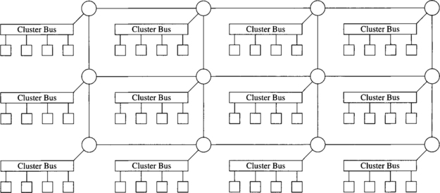
Other combinations are possible. Instead of combining buses and direct networks, the HP/Convex Exemplar multiprocessor combines indirect and direct networks. This multiprocessor has 5 × 5 nonblocking crossbars at the lower level in the hierarchy, connecting four functional blocks and one I/O interface to form clusters or hypernodes. Each functional block consists of two processors, two memory banks, and interfaces. These hypernodes are connected by a second-level coherent toroidal interconnect made out of multiple rings using Scalable Coherent Interface (SCI). Each ring connects one functional block from all the hypernodes. At the lower level of the hierarchy, the crossbars allow all the processors within a hypernode to access the interleaved memory modules in that hypernode. At the higher level, the rings implement a cache coherence protocol.
1.8.4 Other Hypergraph Topologies
Many other hybrid topologies have been proposed [25, 337, 349]. Among them, a particularly interesting class is the hypermesh [336]. A hypermesh is a regular topology consisting of a set of nodes arranged into several dimensions. Instead of having direct connections to the neighbors in each dimension, each node is connected to all the nodes in each dimension through a bus. There are several ways to implement a hypermesh. The most straightforward way consists of connecting all the nodes in each dimension through a shared bus. Figure 1.27 shows a 2-D hypermesh. In this network, multiple buses are arranged in two dimensions. Each node is connected to one bus in each dimension. This topology was proposed by Wittie [349] and was referred to as a spanning-bus hypercube. This topology has a very low diameter, and the average distance between nodes scales very well with network size. However, the overall network bandwidth does not scale well. Additionally, the frequent changes of bus mastership incur significant overheads.
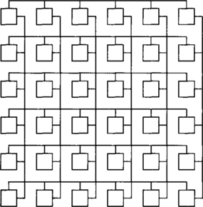
An alternative implementation that removes the above-mentioned constraints consists of replacing the single shared bus connecting the nodes along a given dimension by a set of as many buses as nodes in that dimension. This is the approach proposed in the Distributed Crossbar Switch Hypermesh (DCSH) [222, 223]. Figure 1.28 shows one dimension of the network. Each bus is driven by a single node. Therefore, there are no changes in mastership. Also, bandwidth scales with the number of nodes. Two major concerns, however, are the high number of buses required in the system and the very high number of input ports required at each node. Although the authors propose an electrical implementation, this topology is also suitable for optical interconnects.
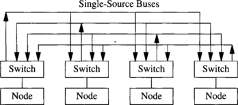
1.9 A Unified View of Direct and Indirect Networks
Up to this point, most researchers and manufacturers considered direct and indirect networks as two completely different approaches for the interconnection of a set of nodes.
However, the last few years have seen developments in router architecture, algorithms, and switch design evolve to a point that is blurring the distinction between these two classes of networks. For performance-driven environments, as networks converge on the use of pipelined message transmission and source-based routing algorithms, the major differences between the switch architectures for direct and indirect networks are becoming more a question of topology. Direct networks have typically used routers with routing algorithms implemented in the network. Switch-based designs have had routing performed at the source. Modern routers are being designed to support simple, fast, reprogrammable routing decisions within the network with substantial control of routing at the message source. This expands the base of applications for the (sizeable) investment in router/switch designs. This flexibility is also evidenced by the fact that the traditional high-performance multiprocessor router/switch designs are moving up to implementations involving workstation and personal computer clusters.
In particular, during the last few years several manufacturers have introduced switches to interconnect a set of processors. These switch-based networks allow the user to define the topology. Let us consider the particular case in which each switch has a single processor directly attached to it, and the remaining ports are used to connect with other switches. This network does not differ substantially from a direct network because each switch can be considered as a router associated with the corresponding node. Indeed, the functionality of current routers and switches is practically identical. Moreover, some manufacturers proposed the use of the same switch to implement either direct or indirect networks. This is the case of the Inmos C 104 switch [228] and the SGI SPIDER [117]. For interconnection networks using the former switch, Inmos proposed the use of bidirectional multistage interconnection networks as well as direct topologies like meshes. In the latter case, each switch is connected to a single node through a set of independent ports. Also, two adjacent switches may use several ports in parallel to communicate between them. The SGI SPIDER router implementation was designed to support configurations as nonblocking multistage networks, as irregular topologies, and as routers for conventional multiprocessor topologies. Such flexibility is typically achieved using topology-independent routing algorithms and flexible switching techniques.
Therefore, we can view networks using point-to-point links as a set of interconnected switches, each one being connected to zero, one, or more nodes. Direct networks correspond to the case where every switch is connected to a single node. Crossbar networks correspond to the case where there is a single switch connected to all the nodes. Multistage interconnection networks correspond to the case where switches are arranged into several stages and the switches in intermediate stages are not connected to any processor. However, other choices are possible under this unified view of direct and indirect interconnection networks. Effectively, nothing prevents the designer from interconnecting switches using a typical direct network topology and connecting several processors to each switch. This is the case for the Cray T3D, which implements a 3-D torus topology, connecting two processors to each router.
The unified view allows the development of generic routing algorithms. In these algorithms, the destination address specifies the destination switch as well as the port number in that switch that is connected to the destination processor. Note that routing algorithms for direct networks are a particular case of these generic algorithms. In this case, there is a single processor connected to each switch. So, the output port in the last switch is not required, assuming that processors are connected to the same port in every switch. This unified view also allows the application of many results developed for direct networks to indirect networks, and vice versa. For example, the theory of deadlock avoidance presented in Chapter 3 was initially developed for direct networks but can also be applied to indirect networks with minor changes, as will be shown in that chapter. Obviously, not all the results can be directly applied to both network classes. Additionally, applying some results to other network classes may require a considerable effort. In the remaining chapters of the book, most techniques will be described for the class of networks for which they were initially proposed. However, it is important to keep in mind that most of those techniques can also be applied to other network topologies by taking into account the unified view proposed in this section.