
Performance Evaluation
This chapter studies the performance of interconnection networks, analyzing the effect of network traffic and the impact of many design parameters discussed in previous chapters. Whenever possible, suggestions will be given for some design parameters. However, we do not intend to study the whole design space. Therefore, this chapter also presents general aspects of network evaluation, so that you can evaluate the effect of parameters that are not considered in this chapter.
As indicated in Chapter 8, a high percentage of the communication latency in multicomputers is produced by the overhead in the software messaging layer. At first glance, it may seem that spending time in improving the performance of the interconnection network hardware is useless. However, for very long messages, communication latency is still dominated by the network hardware latency. In this case, networks with a higher channel bandwidth may achieve a higher performance. On the other hand, messages are usually sent by the cache controller in distributed, shared-memory multiprocessors with coherent caches. In this architecture there is no software messaging layer. Therefore, the performance of the interconnection network hardware is much more critical. As a consequence, in this chapter we will mainly evaluate the performance of the interconnection network hardware. We will consider the overhead of the software messaging layer in Section 9.12.
Network load has a very strong influence on performance. In general, for a given distribution of destinations, the average message latency of a wormhole-switched network is more heavily affected by network load than by any design parameter, provided that a reasonable choice is made for those parameters. Also, throughput is heavily affected by the traffic pattern (distribution of destinations). Therefore, modeling the network workload is very important. Most performance evaluation results have only considered a uniform distribution of message destinations. However, several researchers have considered other synthetic workloads, trying to model the behavior of real applications. Up to now, very few researchers have evaluated networks using the traffic patterns produced by real applications. Therefore, in this chapter we will mainly present results obtained by using synthetic workloads.
Most evaluation results presented in this chapter do not consider the impact of design parameters on clock frequency. However, some design choices may considerably increase router complexity, therefore reducing clock frequency accordingly. Router delay is mostly affected by the number of dimensions of the network, the routing algorithm, and the number of virtual channels per physical channel. The evaluation presented in Section 9.10 considers a very detailed model, trying to be as close as possible to the real behavior of the networks. As will be seen, conclusions are a bit different when the impact of design parameters on clock frequency is considered.
In addition to unicast messages, many parallel applications perform some collective communication operations. Providing support for those operations may reduce latency significantly. Collective communication schemes range from software approaches based on unicast messages to specific hardware support for multidestination messages. These schemes are evaluated in Section 9.11.
Finally, most network evaluations only focus on performance. However, reliability is also important. A wide spectrum of routing protocols has been proposed to tolerate faulty components in the network, ranging from software approaches for wormhole switching to very resilient mechanisms based on different switching techniques. Thus, we will also present some results concerning network fault tolerance in Section 9.13.
9.1 Performance Metrics and Normalized Results
This section introduces performance metrics and defines some standard ways to illustrate performance results. In the absence of faults, the most important performance metrics of an interconnection network are latency and throughput.
Latency is the time elapsed from when the message transmission is initiated until the message is received at the destination node. This general definition is vague and can be interpreted in different ways. If the study only considers the network hardware, latency is usually defined as the time elapsed from when the message header is injected into the network at the source node until the last unit of information is received at the destination node. If the study also considers the injection queues, the queuing time at the source node is added to the latency. This queuing time is usually negligible unless the network is close to its saturation point. When the messaging layer is also being considered, latency is defined as the time elapsed from when the system call to send a message is initiated at the source node until the system call to receive that message returns control to the user program at the destination node.
Latency can also be defined for collective communication operations. In this case, latency is usually measured from when the operation starts at some node until all the nodes involved in that operation have completed their task. For example, when only the network hardware is being considered, the latency of a multicast operation is the time elapsed from when the first fragment of the message header is injected into the network at the source node until the last unit of information is received at the last destination node.
The latency of individual messages is not important, especially when the study is performed using synthetic workloads. In most cases, the designer is interested in the average value of the latency. The standard deviation is also important because the execution time of parallel programs may increase considerably if some messages experience a much higher latency than the average value. A high value of the standard deviation usually indicates that some messages are blocked for a long time in the network. The peak value of the latency can also help in identifying these situations.
Latency is measured in time units. However, when comparing several design choices, the absolute value is not important. As many comparisons are performed by using network simulators, latency can be measured in simulator clock cycles. Unless otherwise stated, the latency plots presented in this chapter for unicast messages measure the average value of the time elapsed from when the message header is injected into the network at the source node until the last unit of information is received at the destination node. In most cases, the simulator clock cycle is the unit of measurement. However, in Section 9.10, latency is measured in nanoseconds.
Throughput is the maximum amount of information delivered per time unit. It can also be defined as the maximum traffic accepted by the network, where traffic, or accepted traffic is the amount of information delivered per time unit. Throughput could be measured in messages per second or messages per clock cycle, depending on whether absolute or relative timing is used. However, throughput would depend on message and network size. So, throughput is usually normalized, dividing it by message size and network size. As a result, throughput can be measured in bits per node and microsecond, or in bits per node and clock cycle. Again, when comparing different design choices by simulation, and assuming that channel width is equal to flit size, throughput can be measured in flits per node and clock cycle. Alternatively, accepted traffic and throughput can be measured as a fraction of network capacity. A uniformly loaded network is operating at capacity if the most heavily loaded channel is used 100% of the time [72]. Again, network capacity depends on the communication pattern.
A standard way to measure accepted traffic and throughput was proposed at the Workshop on Parallel Computer Routing and Communication (PCRCW’94). It consists of representing them as a fraction of the network capacity for a uniform distribution of destinations, assuming that the most heavily loaded channels are located in the network bisection. This network capacity is referred to as normalized bandwidth. So, regardless of the communication pattern used, it is recommended to measure applied load, accepted traffic, and throughput as a fraction of normalized bandwidth. Normalized bandwidth can be easily derived by considering that 50% of uniform random traffic crosses the bisection of the network. Thus, if a network has bisection bandwidth B bits/s, each node in an N-node network can inject 2B/N bits/s at the maximum load. Unless otherwise stated, accepted traffic and throughput are measured as a fraction of normalized bandwidth. While this is acceptable when comparing different design choices in the same network, it should be taken into account that those choices may lead to different clock cycles. In this case, each set of design parameters may produce a different bisection bandwidth, therefore invalidating the normalized bandwidth as a traffic unit. In that case, accepted traffic and throughput can be measured in bits (flits) per node and microsecond. We use this unit in Section 9.10.
A common misconception consists of using throughput instead of traffic. As mentioned above, throughput is the maximum accepted traffic. Another misconception consists of considering throughput or traffic as input parameters instead of measurements, even representing latency as a function of traffic. When running simulations with synthetic workloads, the applied load (also known as offered traffic, generation rate, or injection rate) is an input parameter while latency and accepted traffic are measurements. So, latency-traffic graphs do not represent functions. It should be noted that the network may be unstable when accepted traffic reaches its maximum value. In this case, increasing the applied load may reduce the accepted traffic until a stable point is reached. As a consequence, for some values of the accepted traffic there exist two values for the latency, clearly indicating that the graph does not represent a function.
In the presence of faults, both performance and reliability are important. When presenting performance plots, the Chaos Normal Form (CNF) format (to be described below) should be preferred in order to analyze accepted traffic as a function of applied load. Plots can be represented for different values of the number of faults. In this case, accepted traffic can be smaller than applied load because the network is saturated or because some messages cannot be delivered in the presence of faults. Another interesting measure is the probability of message delivery as a function of the number of failures.
The next sections describe two standard formats to represent performance results. These formats were proposed at PCRCW’94. The CNF requires paired accepted traffic versus applied load and latency versus applied load graphs. The Burton Normal Form (BNF) uses a single latency versus accepted traffic graph. Use of only latency (including source queuing) versus applied load is discouraged because it is impossible to gain any data about performance above saturation using such graphs.
Chaos Normal Form (CNF)
CNF graphs display accepted traffic on one graph and network latency on a second graph. In both graphs, the X-axis corresponds to normalized applied load. By using two graphs, the latency is shown both below and above saturation, and the accepted traffic above saturation is visible. While BNF graphs show the same data, CNF graphs are more clear in their presentation of the data.
Burton Normal Form (BNF)
BNF graphs, advocated by Burton Smith, provide a single-graph plot of both latency and accepted traffic. The X-axis corresponds to accepted traffic, and the Y-axis corresponds to latency. Because the X-axis is a dependent variable, the resulting plot may not be a function. This causes the graph to be a bit hard to comprehend at first glance.
9.2 Workload Models
The evaluation of interconnection networks requires the definition of representative workload models. This is a difficult task because the behavior of the network may differ considerably from one architecture to another and from one application to another. For example, some applications running in multicomputers generate very long messages, while distributed, shared-memory multiprocessors with coherent caches generate very short messages. Moreover, in general, performance is more heavily affected by traffic conditions than by design parameters.
Up to now, there has been no agreement on a set of standard traces that could be used for network evaluation. Most performance analysis used synthetic workloads with different characteristics. In what follows, we describe the most frequently used workload models. These models can be used in the absence of more detailed information about the applications.
The workload model is basically defined by three parameters: distribution of destinations, injection rate, and message length. The distribution of destinations indicates the destination for the next message at each node. The most frequently used distribution is the uniform one. In this distribution, the probability of node i sending a message to node j is the same for all i and j, i ≠ j [288]. The case of nodes sending messages to themselves is excluded because we are interested in message transfers that use the network. The uniform distribution makes no assumptions about the type of computation generating the messages. In the study of interconnection networks, it is the most frequently used distribution. The uniform distribution provides what is likely to be an upper bound on the mean internode distance because most computations exhibit some degree of communication locality.
Communication locality can be classified as spatial or temporal [288]. An application exhibits spatial locality when the mean internode distance is smaller than in the uniform distribution. As a result, each message consumes less resources, also reducing contention. An application has temporal locality when it exhibits communication affinity among a subset of nodes. As a consequence, the probability of sending messages to nodes that were recently used as destinations for other messages is higher than for other nodes. It should be noted that nodes exhibiting communication affinity need not be near one another in the network.
When network traffic is not uniform, we would expect any reasonable mapping of a parallel computation to place those tasks that exchange messages with high frequency in close physical locations. Two simple distributions to model spatial locality are the sphere of locality and the decreasing probability distribution [288], In the former, a node sends messages to nodes inside a sphere centered on the source node with some usually high probability φ, and to nodes outside the sphere with probability 1 − φ. All the nodes inside the sphere have the same probability of being reached. The same occurs for the nodes outside the sphere. It should be noted that when the network size varies, the ratio between the number of nodes inside and outside the sphere is not constant. This distribution models the communication locality typical of programs solving structured problems (e.g., the nearest-neighbor communication typical of iterative partial differential equation solvers coupled with global communication for convergence checking). In practice, the sphere can be replaced by other geometric figures depending on the topology. For example, it could become a square or a cube in 2-D and 3-D meshes, respectively.
In the decreasing probability distribution, the probability of sending a message to a node decreases as the distance between the source and destination nodes increases. Reed and Grunwald [288] proposed the distribution function Φ(d) = Decay(l, dmax) × ld, 0 < l < 1, where d is the distance between the source and destination nodes, dmax is the network diameter, and l is a locality parameter. Decay (l, dmax) is a normalizing constant for the probability Φ, chosen such that the sum of the probabilities is equal to one. Small values of the locality parameter l mean a high degree of locality; larger values of l mean that messages can travel larger distances. In particular, when l is equal to 1/e, we obtain an exponential distribution. As l approaches one, the distribution function Φ approaches the uniform distribution. Conversely, as l approaches zero, Φ approaches a nearest-neighbor communication pattern. It should be noted that the decreasing probability distribution is adequate for the analysis of networks of different sizes. Simply, Decay (l, dmax) should be computed for each network.
The distributions described above exhibit different degrees of spatial locality but have no temporal locality. Recently, several specific communication patterns between pairs of nodes have been used to evaluate the performance of interconnection networks: bit reversal, perfect shuffle, butterfly, matrix transpose, and complement. These communication patterns take into account the permutations that are usually performed in parallel numerical algorithms [175, 200, 239]. In these patterns, the destination node for the messages generated by a given node is always the same. Therefore, the utilization factor of all the network links is not uniform. However, these distributions achieve the maximum degree of temporal locality. These communication patterns can be defined as follows:
![]() Bit reversal. The node with binary coordinates an−1, an−2, …,a1, a0 communicates with the node a0, a1, …, an−2, an−1.
Bit reversal. The node with binary coordinates an−1, an−2, …,a1, a0 communicates with the node a0, a1, …, an−2, an−1.
![]() Perfect shuffle. The node with binary coordinates an−1, an−2, …, a1, a0 communicates with the node an−2, an−3, …, a0, an−1 (rotate left 1 bit).
Perfect shuffle. The node with binary coordinates an−1, an−2, …, a1, a0 communicates with the node an−2, an−3, …, a0, an−1 (rotate left 1 bit).
![]() Butterfly. The node with binary coordinates an−1, an−2, …, a1, a0 communicates with the node a0, an−2, …, a1, an−1 (swap the most and least significant bits).
Butterfly. The node with binary coordinates an−1, an−2, …, a1, a0 communicates with the node a0, an−2, …, a1, an−1 (swap the most and least significant bits).
![]() Matrix transpose. The node with binary coordinates an−1, an−2, …, a1, a0communicates with the node
Matrix transpose. The node with binary coordinates an−1, an−2, …, a1, a0communicates with the node ![]() .
.
![]() Complement. The node with binary coordinates an−1, an−2, …, a1, a0 communicates with the node
Complement. The node with binary coordinates an−1, an−2, …, a1, a0 communicates with the node ![]() .
.
Finally, a distribution based on a least recently used stack model has been proposed in [288] to model temporal locality. In this model, each node has its own stack containing the m nodes that were most recently sent messages. For each position in the stack there is a probability of sending a message to the node in that position. The sum of probabilities for nodes in the stack is less than one. Therefore, a node not currently in the stack may be chosen as the destination for the next transmission. In this case, after sending the message, its destination node will be included in the stack, replacing the least recently used destination.
For synthetic workloads, the injection rate is usually the same for all the nodes. In most cases, each node is chosen to generate messages according to an exponential distribution. The parameter λ of this distribution is referred to as the injection rate. Other possible distributions include a uniform distribution within an interval, bursty traffic, and traces from parallel applications. For the uniform distribution, the injection rate is the mean value of the interval. Bursty traffic can be generated either by injecting a burst of messages every time a node has to inject information into the network or by changing the injection rate periodically.
The network may use some congestion control mechanism. This mechanism can be implemented by placing a limit on the size of the buffer on the injection channels [36], by restricting injected messages to use some predetermined virtual channel(s) [73], or by waiting until the number of free output virtual channels at a node is higher than a threshold [220]. If a congestion control mechanism is used, the effective injection rate is limited when the network approaches the saturation point. This situation should be taken into account when analyzing performance graphs.
Message length can also be modeled in different ways. In most simulation runs, message length is chosen to be fixed. In this case, message length may be varied from one run to another in order to study the effect of message length. Also, message length can be computed according to a normal distribution or a uniform distribution within an interval. In some cases, it is interesting to analyze the mutual effect of messages with very different lengths. For example, injecting even a small fraction of very long messages into the network may increase the latency of some short messages considerably, therefore increasing the standard deviation of latency. In these cases, a weighted mix of short and long messages should be used. Both short and long messages may be of fixed size, or be normally or uniformly distributed as indicated above. Finally, it should be noted that message length has a considerable influence on network performance. So, the selected message length distribution should be representative of the intended applications. Obviously, application traces should be used if available.
In addition to the workload parameters described above, collective communication requires the generation of the set of nodes involved in each collective communication operation. The number of nodes involved in the operation may be fixed or randomly generated. Once the number of nodes has been determined, node addresses can be computed according to any of the models described above. For example, a multicast operation may start by computing the number of destinations using some statistical distribution. Then, the address of each destination can be computed according to a uniform distribution. Although most performance analyses have been performed by executing only collective communication operations, both unicast messages and multidestination messages coexist in real traffic. Therefore, workload models for collective communication operations should consider a mixture of unicast and multidestination messages. Both the percentage of multidestination messages and the number of nodes involved in the collective communication operation should match as much as possible the characteristics of the intended applications.
9.3 Comparison of Switching Techniques
In this section, we compare the performance of several switching techniques. In particular, we analyze the performance of networks using packet switching, VCT switching, and wormhole switching. Previous comparisons [294] showed that VCT and wormhole switching achieve similar latency for low loads. For packet switching, latency is much higher. On the other hand, VCT and packet switching achieve similar throughput. This throughput is more than twice the value achieved by wormhole switching, which saturates at a lower applied load.
In this section, we take into account the effect of adding virtual channels. We will mainly focus on the comparison between VCT and wormhole switching. As mentioned in Chapter 2, routers implementing wormhole switching are simpler and can be clocked at a higher frequency. In this comparison, we are not taking into account the impact of the delay of router components on clock frequency. However, in order to make the comparison more fair, we assume that VCT and packet switching use edge buffers instead of central buffers. By doing so, the complexity of the flow control hardware is similar for all the switching techniques. Also, as packet switching does not pipeline packet transmission, it is assumed that there are no output buffers, transmitting data directly from an input edge buffer through the switch to the corresponding output channel.
For packet switching, we consider edge buffers with capacities of four packets. For VCT, we consider edge buffers with capacities of one, two, and four packets. For wormhole switching, we show the effect of adding virtual channels. The number of virtual channels is varied from one to four. In this comparison, the buffer capacity of each virtual channel is kept constant (4 flits) regardless of the number of virtual channels. Therefore, adding virtual channels also increases the total buffer capacity associated with each physical channel. The effect of adding virtual channels while keeping the total buffer capacity constant will be studied in Sections 9.7.1 and 9.10.5. The total buffer capacity per physical channel is equal to one packet when using four virtual channels. Note that a blocked packet will span four channels in wormhole switching regardless of the number of virtual channels used. Total buffer capacity will differ from one plot to another. The remaining router parameters (routing time, channel bandwidth, etc.) are the same for all the switching techniques.
Figure 9.1 shows the average packet latency versus normalized accepted traffic for different switching techniques on a 16 × 16 mesh using dimension-order routing, 16-flit packets, and a uniform distribution of message destinations. As expected from the expressions for the base latency in Chapter 2, VCT and wormhole switching achieve the same latency for low traffic. This latency is much lower than the one for packet switching. However, when traffic increases, wormhole switching without virtual channels quickly saturates the network, resulting in low channel utilization.
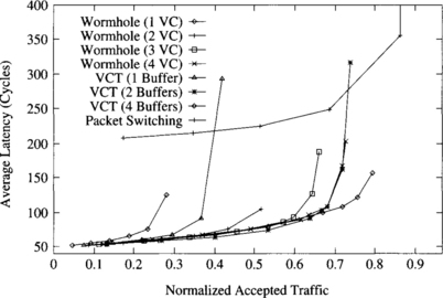
Figure 9.1 Average packet latency versus normalized accepted traffic on a 16 × 16 mesh for different switching techniques and buffer capacities. (VC = virtual channel; VCT = virtual cut-through.)
The low channel utilization of wormhole switching can be improved by adding virtual channels. As virtual channels are added, network throughput increases accordingly. As shown in [72], adding more virtual channels yields diminishing returns. Similarly, increasing queue size for VCT switching also increases throughput considerably. An interesting observation is that the average latency for VCT and for wormhole switching with virtual channels is almost identical for the entire range of applied load until one of the curves reaches the saturation point. Moreover, when the total buffer capacity per physical channel is the same as in VCT, wormhole switching with virtual channels achieves a much higher throughput. It should be noted that in this case wormhole switching uses four virtual channels. However, VCT switching has capacity for a single packet per physical channel. Thus, the channel remains busy until the packet is completely forwarded. Although blocked packets in wormhole switching span multiple channels, the use of virtual channels allow other packets to pass blocked packets.
When VCT switching is implemented by using edge queues with capacity for several packets, channels are freed after transmitting each packet. Therefore, a blocked packet does not prevent the use of the channel by other packets. As a consequence, network throughput is higher than the one for wormhole switching with four virtual channels. Note, however, that the improvement is relatively small, despite the fact that the total buffer capacity for VCT switching is two or four times the buffer capacity for wormhole switching. In particular, we obtained the same results for wormhole switching with four virtual channels and VCT switching with two buffers per channel. We also run simulations for longer packets, keeping the size of the flit buffers used in wormhole switching. In this case, results are more favorable to VCT switching, but buffer requirements also increase accordingly.
Finally, when the network reaches the saturation point, VCT switching has to buffer packets very frequently, therefore preventing pipelining. As a consequence, VCT and packet switching with the same number of buffers achieve similar throughput when the network reaches the saturation point.
The most important conclusion is that wormhole switching is able to achieve latency and throughput comparable to those of VCT switching, provided that enough virtual channels are used and total buffer capacity is similar. If buffer capacity is higher for VCT switching, then this switching technique achieves better performance, but the difference is small if enough virtual channels are used in wormhole switching. These conclusions differ from the ones obtained in previous comparisons because virtual channels were not considered [294]. An additional advantage of wormhole switching is that it is able to handle messages of any size without splitting them into packets. However, VCT switching limits packet size, especially when buffers are implemented in hardware.
As we will see in Section 9.10.5, adding virtual channels increases router delay, decreasing clock frequency accordingly. However, similar considerations can be made when adding buffer space for VCT switching. In what follows we will focus on networks using wormhole switching unless otherwise stated.
9.4 Comparison of Routing Algorithms
In this section we analyze the performance of deterministic and adaptive routing algorithms on several topologies under different traffic conditions. The number of topologies and routing algorithms proposed in the literature is so high that it could take years to evaluate all of them. Therefore, we do not intend to present an exhaustive evaluation. Instead, we will focus on a few topologies and routing algorithms, showing the methodology that can be applied to obtain some preliminary evaluation results. These results are obtained by simulating the behavior of the network under synthetic loads. A detailed evaluation requires the use of representative traces from intended applications.
Most current multicomputers and multiprocessors use low-dimensional (2-D or 3-D) meshes (Intel Paragon [164], Stanford DASH [203], Stanford FLASH [192], MIT Alewife [4], MIT J-Machine [256], MIT Reliable Router [74]) or tori (Cray T3D [259], Cray T3E [313]). Therefore, we will use 2-D and 3-D meshes and tori for the evaluation presented in this section. Also, most multicomputers and multiprocessors use dimension-order routing. However, fully adaptive routing has been recently introduced in both experimental and commercial machines. This is the case for the MIT Reliable Router and the Cray T3E. These routing algorithms are based on the design methodology presented in Section 4.4.4. Therefore, the evaluation presented in this section analyzes the behavior of dimension-order routing algorithms and fully adaptive routing algorithms requiring two sets of virtual channels: one set for dimension-order routing and another set for fully adaptive minimal routing. We also include some performance results for true fully adaptive routing algorithms based on deadlock recovery techniques.
A brief description of the routing algorithms follows. The deterministic routing algorithm for meshes crosses dimensions in increasing order. It does not require virtual channels. When virtual channels are used, the first free virtual channel is selected. The fully adaptive routing algorithm for meshes was presented in Example 3.8. When there are several free output channels, preference is given to the fully adaptive channel in the lowest useful dimension, followed by adaptive channels in increasing useful dimensions. When more than two virtual channels are used, all the additional virtual channels allow fully adaptive routing. In this case, virtual channels are selected in such a way that channel multiplexing is minimized. The deterministic routing algorithm for tori requires two virtual channels per physical channel. It was presented in Example 4.1 for unidirectional channels. The algorithm evaluated in this section uses bidirectional channels. When more than two virtual channels are used, every pair of additional channels has the same routing functionality as the first pair. As this algorithm produces a low channel utilization, we also evaluate a dimension-order routing algorithm that allows a higher flexibility in the use of virtual channels. This algorithm is based on the extension of the routing algorithm presented in Example 3.3 for unidirectional rings. The extended algorithm uses bidirectional channels following minimal paths. Also, dimensions are crossed in ascending order. This algorithm will be referred to as “partially adaptive” because it offers two routing choices for many destinations. The fully adaptive routing algorithm for tori requires one additional virtual channel for fully adaptive minimal routing. The remaining channels are used as in the partially adaptive algorithm. This algorithm was described in Exercise 4.4. Again, when there are several free output channels, preference is given to the fully adaptive channel in the lowest useful dimension, followed by adaptive channels in increasing useful dimensions. When more than two virtual channels are used, all the additional virtual channels allow fully adaptive routing. In this case, virtual channels are selected in such a way that channel multiplexing is minimized. Finally, the true fully adaptive routing algorithm allows fully adaptive minimal routing on all the virtual channels. Again, virtual channels are selected in such a way that channel multiplexing is minimized. This algorithm was described in Section 4.5.3. Deadlocks may occur and are handled by using Disha (see Section 3.6).
Unless otherwise stated, simulations were run using the following parameters. It takes one clock cycle to compute the routing algorithm, to transfer one flit from an input buffer to an output buffer, or to transfer one flit across a physical channel. Input and output flit buffers have a variable capacity, so that the total buffer capacity per physical channel is kept constant. Each node has four injection and four delivery channels. Also, unless otherwise stated, message length is kept constant and equal to 16 flits (plus 1 header flit).
9.4.1 Performance under Uniform Traffic
In this section, we evaluate the performance of several routing algorithms by using a uniform distribution for message destinations.
Deterministic versus Adaptive Routing
Figure 9.2 shows the average message latency versus normalized accepted traffic on a 2-D mesh when using a uniform distribution for message destinations. The graph shows the performance of deterministic routing with one and two virtual channels and of fully adaptive routing (with two virtual channels). As can be seen, the use of two virtual channels almost doubles the throughput of the deterministic routing algorithm. The main reason is that when messages block, channel bandwidth is not wasted because other messages are allowed to use that bandwidth. Therefore, adding a few virtual channels reduces contention and increases channel utilization. The adaptive algorithm achieves 88% of the throughput achieved by the deterministic algorithm with the same number of virtual channels. However, latency is almost identical, being slightly lower for the adaptive algorithm. So, the additional flexibility of fully adaptive routing is not able to improve performance when traffic is uniformly distributed. The reason is that the network is almost uniformly loaded. Additionally, meshes are not regular, and adaptive algorithms tend to concentrate traffic in the central part of the network bisection, thus reducing channel utilization in the borders of the mesh.
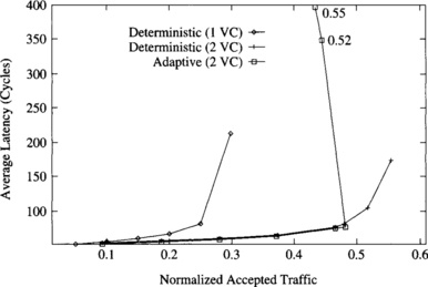
Figure 9.2 Average message latency versus normalized accepted traffic on a 16 × 16 mesh for a uniform distribution of message destinations.
It should be noted that there is a small performance degradation when the adaptive algorithm reaches the saturation point. If the injection rate is sustained at this point, latency increases considerably while accepted traffic decreases. This behavior is typical of routing algorithms that allow cyclic dependencies between channels and will be studied in Section 9.9.
Figure 9.3 shows the average message latency versus normalized accepted traffic on a 3-D mesh when using a uniform distribution for message destinations. This graph is quite similar to the one for 2-D meshes. However, there are some significant differences. The advantages of using two virtual channels in the deterministic algorithm are more noticeable on 3-D meshes. In this case, throughput is doubled. Also, the fully adaptive algorithm achieves the same throughput as the deterministic algorithm with the same number of virtual channels. The latency reduction achieved by the fully adaptive routing algorithm is also more noticeable on 3-D meshes. The reason is that messages have an additional channel to choose from at most intermediate nodes. Again, there is some performance degradation when the adaptive algorithm reaches the saturation point. This degradation is more noticeable than on 2-D meshes.
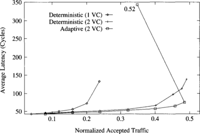
Figure 9.3 Average message latency versus normalized accepted traffic on an 8 × 8 × 8 mesh for a uniform distribution of message destinations.
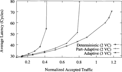
Figure 9.4 shows the average message latency versus normalized accepted traffic on a 2-D torus when using a uniform distribution for message destinations. The graph shows the performance of deterministic routing with two virtual channels, partially adaptive routing with two virtual channels, and fully adaptive routing with three virtual channels.
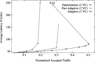
Figure 9.4 Average message latency versus normalized accepted traffic on a 16 × 16 torus for a uniform distribution of message destinations.
Both partially adaptive and fully adaptive algorithms considerably increase performance over the deterministic one. The partially adaptive algorithm increases throughput by 56%. The reason is that channel utilization is unbalanced in the deterministic routing algorithm. However, the partially adaptive algorithm allows most messages to choose between two virtual channels instead of one, therefore reducing contention and increasing channel utilization. Note that the additional flexibility is achieved without increasing the number of virtual channels. The fully adaptive algorithm increases throughput over the deterministic one by a factor of 2.5. This considerable improvement is mainly due to the ability to cross dimensions in any order. Unlike meshes, tori are regular topologies. So, adaptive algorithms are able to improve channel utilization by distributing traffic more uniformly across the network. Partially adaptive and fully adaptive algorithms also achieve a reduction in message latency with respect to the deterministic one for the full range of network load. Similarly, the fully adaptive algorithm reduces latency with respect to the partially adaptive one. However, performance degradation beyond the saturation point reduces accepted traffic to 55% of its maximum value.
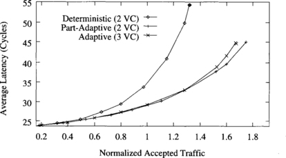
Figure 9.5 shows the average message latency versus normalized accepted traffic on a 3-D torus when using a uniform distribution for message destinations. In addition to the routing algorithms analyzed in Figure 9.4, this graph also shows the performance of the partially adaptive routing algorithm with three virtual channels. Similarly to meshes, adaptive routing algorithms perform comparatively better on a 3-D torus than on a 2-D torus. In this case, the partially adaptive and fully adaptive algorithms increase throughput by factors of 1.7 and 2.6, respectively, over the deterministic one. Latency reduction is also more noticeable than on a 2-D torus. This graph also shows that adding one virtual channel to the partially adaptive algorithm does not improve performance significantly. Although throughput increases by 18%, latency is also increased. The reason is that the partially adaptive algorithm with two virtual channels already allows the use of two virtual channels to most messages, therefore allowing them to share channel bandwidth. So, adding another virtual channel has a small impact on performance. The effect of adding virtual channels will be analyzed in more detail in Section 9.7.1. This result is similar for other traffic distributions. Therefore, in what follows we will only consider the partially adaptive algorithm with two virtual channels. This result also confirms that the improvement achieved by the fully adaptive algorithm is mainly due to the ability to cross dimensions in any order.
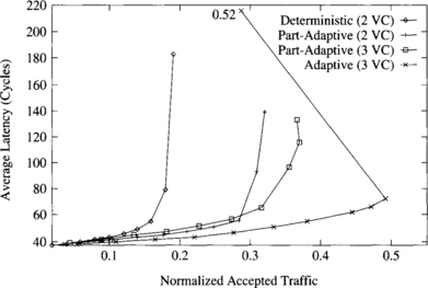
Figure 9.5 Average message latency versus normalized accepted traffic on an 8 × 8 × 8 torus for a uniform distribution of message destinations.
The relative behavior of deterministic and adaptive routing algorithms on 2-D and 3-D meshes and tori when message destinations are uniformly distributed is similar for other traffic distributions. In what follows, we will only present simulation results for a single topology. We have chosen the 3-D torus because most performance results published up to now focus on meshes. So, unless otherwise stated, performance results correspond to a 512-node 3-D torus.
Figure 9.6 shows the standard deviation of latency versus normalized accepted traffic on a 3-D torus when using a uniform distribution for message destinations. The scale for the Y-axis has been selected to make differences more visible. As can be seen, a higher degree of adaptivity also reduces the deviation with respect to the mean value. The reason is that adaptive routing considerably reduces contention at intermediate nodes, making latency more predictable. This occurs in all the simulations we run. So, in what follows, we will only present graphs for the average message latency.
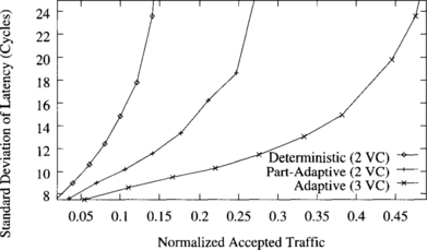
Figure 9.6 Standard deviation of latency versus normalized accepted traffic on an 8 × 8 × 8 torus for a uniform distribution of destinations.
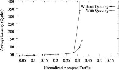
In Figure 9.5, latency is measured from when a message is injected into the network. It does not consider queuing time at the source node. When queuing time is considered, latency should not differ significantly unless the network is close to saturation. When the network is close to saturation, queuing time increases considerably. Figure 9.7 shows the average message latency versus normalized accepted traffic for the partially adaptive algorithm on a 3-D torus. This figure shows that latency is not affected by queuing time unless the network is close to saturation.
Deadlock Avoidance versus Deadlock Recovery
Figure 9.8 plots the average message latency versus normalized accepted traffic for deadlock-recovery-based and avoidance-based deterministic and adaptive routing algorithms. The simulations are based on a 3-D torus (512 nodes) with uniform traffic distribution and 16-flit messages. Each node has a single injection and delivery channel. The timeout used for deadlock detection is 25 cycles. The recovery-based deterministic routing algorithm with two virtual channels is able to use both of the virtual channels without restriction and is therefore able to achieve a 100% improvement in throughput over avoidance-based deterministic routing. Avoidance-based fully adaptive routing is able to achieve a slightly higher throughput and lower latency than recovery-based deterministic routing when using an additional virtual channel. Note that this algorithm allows unrestricted adaptive routing on only one of its three virtual channels. By freely using all three virtual channels, recovery-based true fully adaptive routing is able to achieve a 34% higher throughput than its avoidance-based counterpart.
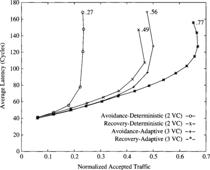
Figure 9.8 Average message latency versus normalized accepted traffic on an 8 × 8 × 8 torus for a uniform distribution of message destinations.
These results show the potential improvement that can be achieved by using deadlock recovery techniques like Disha to handle deadlocks. It should be noted, however, that a single injection/delivery channel per node has been used in the simulations. If the number of injection/delivery channels per node is increased, the additional traffic injected into the network increases the probability of deadlock detection at saturation, and deadlock buffers are unable to recover from deadlock fast enough. Similarly, when messages are long, deadlock buffers are occupied for a long time every time a deadlock is recovered from, thus degrading performance considerably when the network reaches saturation. In this case, avoidance-based adaptive routing algorithms usually achieve better performance than recovery-based algorithms. This does not mean that recovery-based algorithms are not useful as general-purpose routing algorithms. Simply, currently available techniques are not able to recover from deadlock fast enough when messages are long or when several injection/delivery channels per node are used. The main reason is that currently available deadlock detection techniques detect many false deadlocks, therefore saturating the bandwidth provided by the deadlock buffers. However, this situation may change when more powerful techniques for deadlock detection are developed. In what follows, we will only analyze avoidance-based routing algorithms.
9.4.2 Performance under Local Traffic
Figure 9.9 shows the average message latency versus normalized accepted traffic when messages are sent locally. In this case, message destinations are uniformly distributed inside a cube centered at the source node with each side equal to four channels.
The partially adaptive algorithm doubles throughput with respect to the deterministic one when messages are sent locally. The fully adaptive algorithm performs even better, reaching a throughput three times higher than the deterministic algorithm and 50% higher than the partially adaptive algorithm. Latency is also smaller for the full range of accepted traffic.
When locality increases even more, the benefits of using adaptive algorithms are smaller because the distance between source and destination nodes are short, and the number of alternative paths is much smaller. Figure 9.10 shows the average message latency versus normalized accepted traffic when messages are uniformly distributed inside a cube centered at the source node with each side equal to two channels. In this case, partially and fully adaptive algorithms perform almost the same. All the improvement with respect to the deterministic algorithm comes from a better utilization of virtual channels.
9.4.3 Performance under Nonuniform Traffic
As stated in [73], adaptive routing is especially interesting when traffic is not uniform. Figures 9.11 and 9.12 compare the performance of routing algorithms for the bit reversal and perfect shuffle communication patterns, respectively. In both cases, the deterministic and partially adaptive algorithms achieve poor performance because both of them offer a single physical path for every source/destination pair.
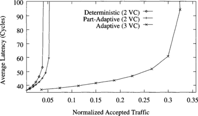
Figure 9.11 Average message latency versus normalized accepted traffic for the bit reversal traffic pattern.
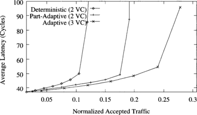
Figure 9.12 Average message latency versus normalized accepted traffic for the perfect shuffle traffic pattern.
The fully adaptive algorithm increases throughput by a factor of 2.25 with respect to the deterministic algorithm when using the perfect shuffle communication pattern, and it increases throughput by a factor of 8 in the bit reversal communication pattern. Standard deviation of message latency is also much smaller for the fully adaptive algorithm. Finally, note that there is no significant performance degradation when the fully adaptive algorithm reaches the saturation point, especially for the perfect shuffle communication pattern.
9.5 Effect of Message Length
In this section we analyze the effect of message length on performance. We will only consider the traffic patterns for which the adaptive algorithm behaves more differently: uniform distribution and very local traffic (side = 2). Figures 9.13 and 9.14 show the average message latency divided by message length for uniform and local traffic, respectively. For the sake of clarity, plots only show the behavior of deterministic and fully adaptive algorithms with short (16-flit) and long (256-flit) messages. We also run simulations for other message lengths. For 64-flit messages, plots were close to the plots for 256-flit messages. For 128-flit messages, plots almost overlapped the ones for 256-flit messages. Similar results were obtained for messages longer than 256 flits.
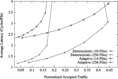
Figure 9.13 Average message latency divided by message length versus normalized accepted traffic for a uniform distribution of message destinations.
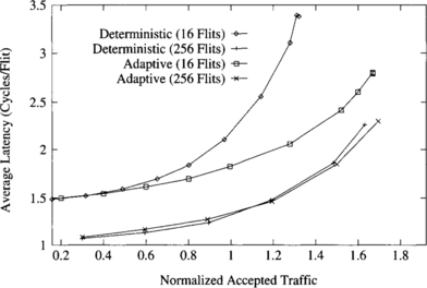
Figure 9.14 Average message latency divided by message length versus normalized accepted traffic for local traffic (side = 2).
The average flit latency is smaller for long messages. The reason is that messages are pipelined. Path setup time is amortized among more flits when messages are long. Moreover, data flits can advance faster than message headers because headers have to be routed, waiting for the routing control unit to compute the output channel, and possibly waiting for the output channel to become free. Therefore, when the header reaches the destination node, data flits advance faster, thus favoring long messages. Throughput is also smaller for short messages when the deterministic algorithm is used. However, the fully adaptive algorithm performs comparatively better for short messages, achieving almost the same throughput for short and long messages. Hence, this routing algorithm is more robust against variations in message size. This is due to the ability of the adaptive algorithm to use alternative paths. As a consequence, header blocking time is much smaller than for the deterministic algorithm, achieving a better channel utilization.
9.6 Effect of Network Size
In this section we study the performance of routing algorithms when network size increases. Figure 9.15 shows the average message latency versus normalized accepted traffic on a 16-ary 3-cube (4,096 nodes) when using a uniform distribution for message destinations.
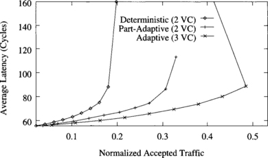
Figure 9.15 Average message latency versus normalized accepted traffic for a uniform distribution of message destinations. Network size = 4K nodes.
The shape of the plots and the relative behavior of routing algorithms are similar to the ones for networks with 512 nodes (Figure 9.5). Although normalized throughput is approximately the same, absolute throughput is approximately half the value obtained for 512 nodes. The reason is that there are twice as many nodes in each dimension and the average distance traveled by each message is doubled. Also, bisection bandwidth increases by a factor of 4 while the number of nodes sending messages across the bisection increases by a factor of 8. However, latency only increases by 45% on average, clearly showing the advantages of message pipelining across the network. In summary, scalability is acceptable when traffic is uniformly distributed. However, the only way to make networks really scalable is by exploiting communication locality.
9.7 Impact of Design Parameters
This section analyzes the impact of several design parameters on network performance: number of virtual channels, number of ports, and buffer size.
9.7.1 Effect of the Number of Virtual Channels
Splitting each physical channel into several virtual channels increases the number of routing choices, allowing messages to pass blocked messages. On the other hand, flits from several messages are multiplexed onto the same physical channel, slowing down both messages. The effect of increasing the number of virtual channels has been analyzed in [72] for deterministic routing algorithms on a 2-D mesh topology.
In this section, we analyze the effect of increasing the number of virtual channels on all the algorithms under study, using a uniform distribution of message destinations. As in [72], we assume that the total buffer capacity associated with each physical channel is kept constant and is equal to 16 flits (15 flits and 18 flits for three and six virtual channels, respectively).
Figure 9.16 shows the behavior of the deterministic algorithm with two, four, six, and eight virtual channels per physical channel. Note that the number of virtual channels for this algorithm must be even. The higher the number of virtual channels, the higher the throughput. However, the highest increment is produced when changing from two to four virtual channels. Also, latency slightly increases when adding virtual channels. These results are very similar to the ones obtained in [72]. The explanation is simple: Adding the first few virtual channels allows messages to pass blocked messages, increasing channel utilization and throughput. Adding more virtual channels does not increase routing flexibility considerably. Moreover, buffer size is smaller, and blocked messages occupy more channels. As a result, throughput increases by a small amount. Adding virtual channels also has a negative effect [88]. Bandwidth is shared among several messages. However, bandwidth sharing is not uniform. A message may be crossing several physical channels with different degrees of multiplexing. The more multiplexed channel becomes a bottleneck, slightly increasing latency.
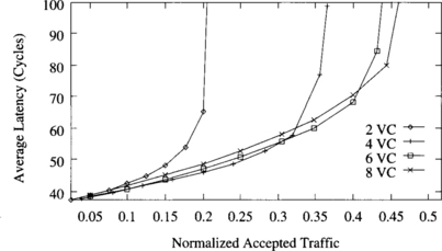
Figure 9.16 Effect of the number of virtual channels on the deterministic algorithm. Plots show the average message latency versus normalized accepted traffic for a uniform distribution of message destinations.
Figure 9.17 shows the behavior of the partially adaptive algorithm with two, four, six, and eight virtual channels. In this case, adding two virtual channels increases throughput by a small amount. However, adding more virtual channels increases latency and even reduces throughput. Moreover, the partially adaptive algorithm with two and four virtual channels achieves almost the same throughput as the deterministic algorithm with four and eight virtual channels, respectively. Note that the partially adaptive algorithm is identical to the deterministic one, except that it allows most messages to share all the virtual channels. Therefore, it effectively allows the same degree of channel multiplexing using half the number of virtual channels as the deterministic algorithm. When more than four virtual channels are used, the negative effects of channel multiplexing mentioned above outweigh the benefits.
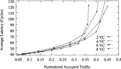
Figure 9.17 Effect of the number of virtual channels on the partially adaptive algorithm. Plots show the average message latency versus normalized accepted traffic for a uniform distribution of message destinations.
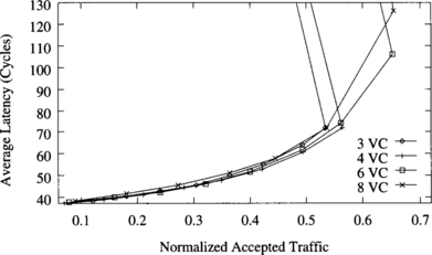
Figure 9.18 shows the behavior of the fully adaptive algorithm with three, four, six, and eight virtual channels. Note that two virtual channels are used for deadlock avoidance and the remaining channels are used for fully adaptive routing. In this case, latency is very similar regardless of the number of virtual channels. Note that the selection function selects the output channel for a message in such a way that channel multiplexing is minimized. As a consequence, channel multiplexing is more uniform and channel utilization is higher, obtaining a higher throughput than the other routing algorithms. As indicated in Section 9.4.1, throughput decreases when the fully adaptive algorithm reaches the saturation point. This degradation can be clearly observed in Figure 9.18. Also, as indicated in [91], it can be seen that increasing the number of virtual channels increases throughput and even removes performance degradation.
9.7.2 Effect of the Number of Ports
Network hardware has become very fast. In some cases, network performance may be limited by the bandwidth available at the source and destination nodes to inject and deliver messages, respectively. In this section, we analyze the effect of that bandwidth. As fully adaptive algorithms achieve a higher throughput, this issue is more critical when adaptive routing is used. Therefore, we will restrict our study to fully adaptive algorithms. Injection and delivery channels are usually referred to as ports. In this study, we assume that each port has a bandwidth equal to the channel bandwidth.
Figure 9.19 shows the effect of the number of ports for a uniform distribution of message destinations. For the sake of clarity, we removed the part of the plots corresponding to the performance degradation of the adaptive algorithm close to saturation. As can be seen, the network interface is a clear bottleneck when using a single port. Adding a second port decreases latency and increases throughput considerably. Adding a third port increases throughput by a small amount, and adding more ports does not modify the performance. It should be noted that latency does not consider source queuing time. When a single port is used, latency is higher because messages block when the header reaches the destination node, waiting for a free port. Those blocked messages remain in the network, therefore reducing channel utilization and throughput.
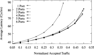
Figure 9.19 Effect of the number of ports for a uniform distribution of message destinations. Plots show the average message latency versus normalized accepted traffic.
As can be expected, more bandwidth is required at the network interface when messages are sent locally. Figure 9.20 shows the effect of the number of ports for local traffic with side = 2 (see Section 9.4.2). In this case, the number of ports has a considerable influence on performance. It has a stronger impact on throughput than the routing algorithm or even the topology used. The higher the number of ports, the higher the throughput. However, as the number of ports increases, adding more ports has a smaller impact on performance. Therefore, in order to avoid mixing the effect of different design parameters, we run all the simulations in the remaining sections of this chapter by using four ports.
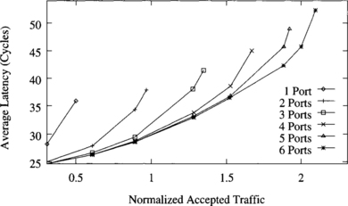
Figure 9.20 Effect of the number of ports for local traffic (side = 2). Plots show the average message latency versus normalized accepted traffic.
Taking into account that the only way to make parallel machines really scalable is by exploiting locality, the effect of the number of ports is extremely important. However, most current multicomputers have a single port. In most cases, the limited bandwidth at the network interface does not limit the performance. The reason is that there is an even more important bottleneck in the network interface: the software messaging layer (see Section 9.12). The latency of the messaging layer reduces network utilization, hiding the effect of the number of ports. However, the number of ports may become the bottleneck in distributed, shared-memory multiprocessors.
9.7.3 Effect of Buffer Size
In this section, we analyze the effect of buffer size on performance. Buffers are required to allow continuous flit injection at the source node in the absence of contention, therefore hiding routing time and allowing windowing protocols between adjacent routers. Also, if messages are short enough, using deeper buffers allows messages to occupy a smaller number of channels when contention arises and buffers are filled. As a consequence, contention is reduced and throughput should increase. Finally, buffers are required to hold flits while a physical channel is transmitting flits from other buffers (virtual channels).
If buffers are kept small, buffer size does not affect clock frequency. However, using very deep buffers may slow down clock frequency, so there is a trade-off. Figure 9.21 shows the effect of input and output buffer size on performance using the fully adaptive routing algorithm with three virtual channels. In this case, no windowing protocol has been implemented. Minimum buffer size is two flits because flit transmission across physical channels is asynchronous. Using smaller buffers would produce bubbles in the message pipeline.
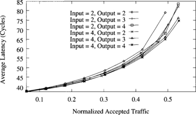
Figure 9.21 Effect of input and output buffer size. Plots show the average message latency versus normalized accepted traffic for the fully adaptive routing algorithm with three virtual channels using a uniform distribution of message destinations.
As expected, the average message latency decreases when buffer size increases. However, the effect of buffer size on performance is small. The only significant improvement occurs when the total flit capacity changes from 4 to 5 flits. Adding more flits to buffer capacity yields diminishing returns as buffer size increases. Increasing input buffer size produces almost the same effect as increasing output buffer size, as far as total buffer size remains the same. The reason is that there is a balance between the benefits of increasing the size of each buffer. On the one hand, increasing the input buffer size allows more data flits to make progress if the routing header is blocked for some cycles until an output channel is available. On the other hand, increasing the output buffer size allows more data flits to cross the switch while the physical channel is assigned to other virtual channels.
Moreover, when a message blocks, buffers are filled. In this case, it does not matter how total buffer capacity is split among input and output buffers. The only important issue is whether buffers are deep enough to allow the blocked message to leave the source node so that some channels are freed.
Note that the plots in Figure 9.21 correspond to short messages (16 flits). We also ran simulations for longer messages. In this case, buffer size has a more noticeable impact on performance. However, increasing buffer capacity does not increase performance significantly if messages are longer than the diameter of the network times the total buffer capacity of a virtual channel. The reason is that a blocked message keeps all the channels it previously reserved regardless of buffer size.
9.8 Comparison of Routing Algorithms for Irregular Topologies
In this section we analyze the performance of the routing algorithms described in Section 4.9 on switch-based networks with randomly generated irregular topologies under uniform traffic. We also study the influence of network size and message length.
A brief description of the routing algorithms follows. A breadth-first spanning tree on the network graph is computed first using a distributed algorithm. Routing is based on an assignment of direction to the operational links. The up end of each link is defined as (1) the end whose switch is closer to the root in the spanning tree or (2) if both ends are at switches at the same tree level, the end whose switch has the lower ID. The up/down routing algorithm uses the following up/down rule: a legal route must traverse zero or more links in the up direction followed by zero or more links in the down direction. We will refer to this routing scheme as UD. It does not require virtual channels. When virtual channels are used, the first free virtual channel is selected. We will refer to the up/down routing scheme in which physical channels are split into two virtual channels as UD-2VC.
The adaptive routing algorithm proposed in [320] also splits each physical channel into two virtual channels (original and new channels). Newly injected messages can use the new channels following any minimal path, but the original channels can only be used according to the up/down rule. However, once a message reserves one of the original channels, it can no longer reserve any of the new channels again. When a message can choose among new and original channels, a higher priority is given to the new channels at any intermediate switch. We will refer to this routing algorithm as A-2VC.
Finally, an enhanced version of the A-2VC algorithm can be obtained as follows [319]: Newly injected messages can only leave the source switch using new channels belonging to minimal paths and never using original channels. When a message arrives at a switch from another switch through a new channel, the routing function gives a higher priority to the new channels belonging to minimal paths. If all of them are busy, then the routing algorithm selects an original channel belonging to a minimal path (if any). If none of the original channels provides minimal routing, then the original channel that provides the shortest path will be used. We will refer to this routing scheme as MA-2VC, since it provides minimal adaptive routing with two virtual channels.
Unless otherwise stated, simulations were run using the following parameters. Network topology is completely irregular and was generated randomly. However, for the sake of simplicity, we imposed three restrictions to the topologies that can be generated. First, we assumed that there are exactly four nodes (processors) connected to each switch. Also, two neighboring switches are connected by a single link. Finally, all the switches in the network have the same size. We assumed eight-port switches, thus leaving four ports available to connect to other switches. We evaluated networks with a size ranging from 16 switches (64 nodes) to 64 switches (256 nodes). For each network size, several distinct irregular topologies were analyzed. However, the average latency values achieved by each topology for each traffic rate were almost the same. The only differences arose when the networks were heavily loaded, close to saturation. Additionally, the throughput achieved by all the topologies was almost the same. Hence, we only show the results obtained by one of those topologies, chosen randomly. Input and output flit buffers have capacity for 4 flits. Each node has one injection and one delivery channel. For message length, 16-, 64-, and 256-flit messages were considered. Finally, it takes one clock cycle to compute the routing algorithm, to transfer one flit from an input buffer to an output buffer, or to transfer one flit across a physical channel.
Note that we assumed that virtual channel multiplexing can be efficiently implemented. In practice, implementing virtual channels is not trivial because switch-based networks with irregular topology are usually used in the context of networks of workstations. In this environment, link wires may be long, increasing signal propagation delay and making flow control more complex.
Figure 9.22 shows the average message latency versus accepted traffic for each routing scheme on a randomly generated irregular network with 16 switches. Message size is 16 flits. It should be noted that accepted traffic has not been normalized because normalized bandwidth differs from one network to another even for the same size. As can be seen, when virtual channels are used in the up/down routing scheme (UD-2VC), throughput increases by a factor of 1.5. The A-2VC routing algorithm doubles throughput and reduces latency with respect to the up/down routing scheme. The improvement with respect to UD-2VC is due to the additional adaptivity provided by A-2VC. When the MA-2VC routing scheme is used, throughput is almost tripled. Moreover, the latency achieved by MA-2VC is lower than the one for the rest of the routing strategies for the whole range of traffic. The improvement achieved by MA-2VC with respect to A-2VC is due to the use of shorter paths. This explains the reduction in latency as well as the increment in throughput because less bandwidth is wasted in nonminimal paths.
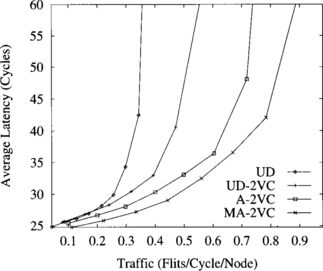
Figure 9.22 Average message latency versus accepted traffic for an irregular network with 16 switches. Message length is 16 flits.
The MA-2VC routing scheme scales very well with network size. Figure 9.23 shows the results obtained on a network with 64 switches. In this network, throughput increases by factors of 4.2 and 2.7 with respect to the UD and UD-2VC schemes, respectively, when using the MA-2VC scheme. Latency is also reduced for the whole range of traffic. However, the factor of improvement in throughput achieved by the A-2VC scheme with respect to UD is only 2.6. Hence, when network size increases, the performance improvement achieved by the MA-2VC scheme also increases because there are larger differences among the minimal distance between any two switches and the routing distance imposed by the up/down routing algorithm.
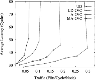
Figure 9.23 Average message latency versus accepted traffic for an irregular network with 64 switches. Message length is 16 flits.
Figures 9.23, 9.24, and 9.25 show the influence of message size on the behavior of the routing schemes. Message size ranges from 16 to 256 flits. As message size increases, the benefits of using virtual channels become smaller. In particular, the UD-2VC routing scheme exhibits a higher latency than the UD scheme for low to medium network traffic. This is due to the fact that when a long message waits for a channel occupied by a long message, it is delayed. However, when two long messages share the channel bandwidth, both of them are delayed. Also, the UD routing scheme increases throughput by a small amount as message size increases. The routing schemes using virtual channels, and in particular the adaptive ones, achieve a similar performance regardless of message size. This behavior matches the one for regular topologies, as indicated in Section 9.5. These results show the robustness of the UD-2VC, A-2VC, and MA-2VC routing schemes against message size variation. Additionally, the MA-2VC routing scheme achieves the highest throughput and lowest latency for all message sizes.
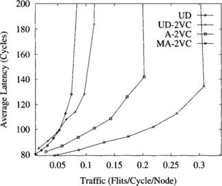
Figure 9.24 Average message latency versus accepted traffic for an irregular network with 64 switches. Message length is 64 flits.
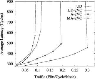
Figure 9.25 Average message latency versus accepted traffic for an irregular network with 64 switches. Message length is 256 flits.
Finally, it should be noted that the improvement achieved by using the theory proposed in Section 3.1.3 for the design of adaptive routing algorithms is much higher in irregular topologies than in regular ones. This is mainly due to the fact that most paths in irregular networks are nonminimal if those techniques are not used.
9.9 Injection Limitation
As indicated in previous sections, the performance of the fully adaptive algorithm degrades considerably when the saturation point is reached. Figure 9.26 shows the average message latency versus normalized accepted traffic for a uniform distribution of message destinations. This plot was already shown in Figure 9.5. Note that each point in the plot corresponds to a stable working point of the network (i.e., the network has reached a steady state). Also, note that Figure 9.26 does not represent a function. The average message latency is not a function of accepted traffic (traffic received at destination nodes). Both average message latency and accepted traffic are functions of the applied load.
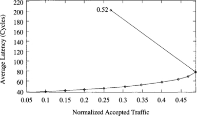
Figure 9.26 Average message latency versus normalized accepted traffic for the fully adaptive algorithm using four ports and a uniform distribution of message destinations.
Figure 9.27 shows the normalized accepted traffic as a function of normalized applied load. As can be seen, accepted traffic increases linearly with the applied load until the saturation point is reached. Indeed, they have the same value because each point corresponds to a steady state. However, when the saturation point is reached, accepted traffic decreases considerably. Further increments of the applied load do not modify accepted traffic. Simply, injection buffers at source nodes grow continuously. Also, average message latency increases by an order of magnitude when the saturation point is reached, remaining constant as applied load increases further. Note that latency does not include source queuing time.
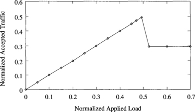
Figure 9.27 Normalized accepted traffic as a function of normalized applied load for the fully adaptive algorithm using four ports and a uniform distribution of message destinations.
This behavior typically arises when the routing algorithm allows cyclic dependencies between resources. As indicated in Chapter 3, deadlocks are avoided by using a subset of channels without cyclic dependencies between them to escape from cyclic waiting chains (escape channels). The bandwidth provided by the escape channels should be high enough to drain messages from cyclic waiting chains as fast as they are formed. The speed at which waiting chains are formed depends on network traffic. The worst case occurs when the network is beyond saturation. At this point congestion is very high. As a consequence, the probability of messages blocking cyclically is not negligible. Escape channels should be able to drain at least one message from each cyclic waiting chain fast enough so that those escape channels are free when they are requested by another possibly deadlocked message. Otherwise, performance degrades and throughput is considerably reduced. The resulting accepted traffic at this point depends on the bandwidth offered by the escape channels.
An interesting issue is that the probability of messages blocking cyclically depends not only on applied load. Increasing the number of virtual channels per physical channel decreases that probability. Reducing the number of injection/delivery ports also decreases that probability. However, those solutions may degrade performance considerably. Also, as indicated in Section 9.4.3, some communication patterns do not produce performance degradation. For those traffic patterns, messages do not block cyclically or do it very infrequently.
The best solution consists of designing the network correctly. A good network design should provide enough bandwidth for the intended applications. The network should not work close to the saturation point because contention at this point is high, increasing message latency and decreasing the overall performance. Even if the network reaches the saturation point for a short period of time, performance will not degrade as much as indicated in Figures 9.26 and 9.27. Note that the points beyond saturation correspond to steady states, requiring a sustained message generation rate higher than the one corresponding to saturation. Moreover, the simulation time required to reach a steady state for those points is an order of magnitude higher than for other points in the plot, indicating that performance degradation does not occur immediately after reaching the saturation point. Also, after reaching the saturation point for some period of time, performance improves again when the message generation rate falls below the value at the saturation point.
If the traffic requirements of the intended applications are not known in advance, it is still possible to avoid performance degradation by using simple hardware mechanisms. A very effective solution consists of limiting message injection when network traffic is high. For efficiency reasons, traffic should be estimated locally. Injection can be limited by placing a limit on the size of the buffer on the injection channels [36], by restricting injected messages to use some predetermined virtual channel(s) [73], or by waiting until the number of free output virtual channels at a node is higher than a threshold [220]. This mechanism can be implemented by keeping a count of the number of free virtual channels at each router. When this count is higher than a given threshold, message injection is allowed. Otherwise, messages have to wait at the source queue. Note that these mechanisms have no relationship with the injection limitation mechanism described in Section 3.3.3. Injection limitation mechanisms may produce starvation if the network works beyond the saturation point for long periods of time.
The injection limitation mechanism described above requires defining a suitable threshold for the number of free output virtual channels. Additionally, this threshold should be independent of the traffic pattern. Figures 9.28, 9.29, and 9.30 show the percentage of busy output virtual channels versus normalized accepted traffic for a uniform distribution, local traffic (side = 2), and the bit reversal traffic pattern, respectively. Interestingly enough, the percentage of busy output virtual channels at the saturation point is similar for all the distributions of destinations. It ranges from 40% to 48%. Other traffic patterns exhibit a similar behavior. Since a 3-D torus with three virtual channels per physical channel has 18 output virtual channels per router, seven or eight virtual channels are occupied. Therefore, 10 or 11 virtual channels are free on average at the saturation point. Thus, messages should only be injected if 11 or more virtual channels are free at the current router. The latency/traffic plots obtained for different traffic patterns when injection is limited are almost identical to the ones without injection limitation, except that throughput does not decrease and latency does not increase beyond the saturation point.
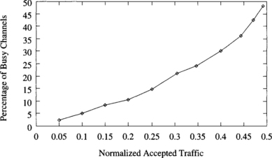
Figure 9.28 Percentage of busy output virtual channels versus normalized accepted traffic for a uniform distribution of message destinations.
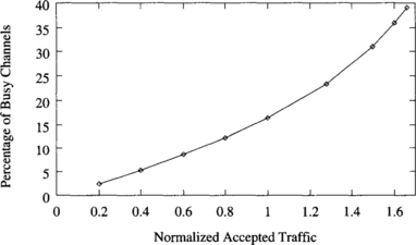
Figure 9.29 Percentage of busy output virtual channels versus normalized accepted traffic for local traffic (side = 2).
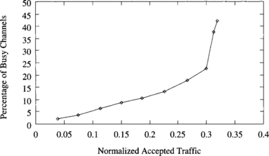
Figure 9.30 Percentage of busy output virtual channels versus normalized accepted traffic for the bit reversal traffic pattern.
Despite the simplicity and effectiveness of the injection limitation mechanism described above, it has not been tried with traffic produced by real applications. Extensive simulations should be run before deciding to include it in a router design. Moreover, if network bandwidth is high enough, this mechanism is not necessary, as indicated above. Nevertheless, new and more powerful injection limitation mechanisms are currently being developed.
9.10 Impact of Router Delays on Performance
In this section, we consider the impact of router and wire delays on performance, using the model proposed in [57].
9.10.1 A Speed Model
Most network simulators written up to now for wormhole switching work at the flit level. Writing a simulator that works at the gate level or at the transistor level is a complex task. Moreover, execution time would be extremely high, considerably reducing the design space that can be studied. A reasonable approximation to study the effect of design parameters on the performance of the interconnection network consists of modeling the delay of each component of the router. Then, for a given set of design parameters, the delay of each component is computed, determining the critical path and the number of clock cycles required for each operation, and computing the clock frequency for the router. Then, the simulation is run using a flit-level simulator. Finally, simulation results are corrected by using the previously computed clock frequency.
Consider the router model described in Section 2.1. We assume that all the operations inside each router are synchronized by its local clock signal. To compute the clock frequency of each router, we will use the delay model proposed in [57]. It assumes 0.8 μm CMOS gate array technology for the implementation.
![]() Routing control unit. Routing a message involves the following operations: address decoding, routing decision, and header selection. The first operation extracts the message header and generates requests of acceptable outputs based on the routing algorithm. In other words, the address decoder implements the routing function. According to [57], the address decoder delay is constant and equal to 2.7 ns. The routing decision logic takes as inputs the possible output channels generated by the address decoder and the status of the output channels. In other words, this logic implements the selection function. This circuit has a delay that grows logarithmically with the number of alternatives, or degrees of freedom, offered by the routing algorithm. Representing the degrees of freedom by F, this circuit has a delay value given by 0.6 + 0.6 log F ns. Finally, the routing control unit must compute the new header, depending on the output channel selected. While new headers can be computed in parallel with the routing decision, it is necessary to select the appropriate one when this decision is made. This operation has a delay that grows logarithmically with the degrees of freedom. Thus, this delay will be 1.4 + 0.6 log F ns. The operations and the associated delays are shown in Figure 9.31. The total routing time will be the sum of all delays, yielding
Routing control unit. Routing a message involves the following operations: address decoding, routing decision, and header selection. The first operation extracts the message header and generates requests of acceptable outputs based on the routing algorithm. In other words, the address decoder implements the routing function. According to [57], the address decoder delay is constant and equal to 2.7 ns. The routing decision logic takes as inputs the possible output channels generated by the address decoder and the status of the output channels. In other words, this logic implements the selection function. This circuit has a delay that grows logarithmically with the number of alternatives, or degrees of freedom, offered by the routing algorithm. Representing the degrees of freedom by F, this circuit has a delay value given by 0.6 + 0.6 log F ns. Finally, the routing control unit must compute the new header, depending on the output channel selected. While new headers can be computed in parallel with the routing decision, it is necessary to select the appropriate one when this decision is made. This operation has a delay that grows logarithmically with the degrees of freedom. Thus, this delay will be 1.4 + 0.6 log F ns. The operations and the associated delays are shown in Figure 9.31. The total routing time will be the sum of all delays, yielding
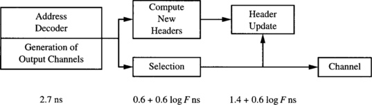
![]() Switch. The time required to transfer a flit from one input channel to the corresponding output channel is the sum of the delay involved in the internal flow control unit, the delay of the crossbar, and the setup time of the output channel latch. The flow control unit manages the buffers, preventing overflow and underflow. It has a constant delay equal to 2.2 ns. The crossbar is usually implemented using a tree of selectors for each output. Thus, its delay grows logarithmically with the number of ports. Assuming that P is the number of ports of the crossbar, its delay is given by 0.4 + 0.6 log P ns. Finally, the setup time of a latch is 0.8 ns. The operations and the associated delays are shown in Figure 9.32. The switch delay is
Switch. The time required to transfer a flit from one input channel to the corresponding output channel is the sum of the delay involved in the internal flow control unit, the delay of the crossbar, and the setup time of the output channel latch. The flow control unit manages the buffers, preventing overflow and underflow. It has a constant delay equal to 2.2 ns. The crossbar is usually implemented using a tree of selectors for each output. Thus, its delay grows logarithmically with the number of ports. Assuming that P is the number of ports of the crossbar, its delay is given by 0.4 + 0.6 log P ns. Finally, the setup time of a latch is 0.8 ns. The operations and the associated delays are shown in Figure 9.32. The switch delay is
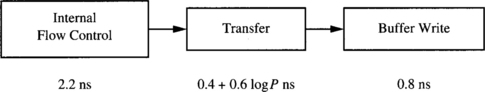
![]() Channels. The time required to transfer a flit across a physical channel includes the off-chip delay across the wires and the time required to latch it onto the destination. Assuming that channel width and flit size are identical, this time is the sum of the output buffer, input buffer, input latch, and synchronizer delays. Typical values for the technology used are 2.5 (with 25 pF load), 0.6, 0.8, and 1.0 ns, respectively, yielding 4.9 ns per flit. The output buffer delay includes the propagation time across the wires, assuming that they are short. This is the case for a 3-D torus when it is assembled in three dimensions. If virtual channels are used, the time required to arbitrate and select one of the ready flits must be added. The virtual channel controller has a delay that grows logarithmically with the number of virtual channels per physical channel. Notice that we do not include any additional delay to decode the virtual channel number at the input of the next node because virtual channels are usually identified using one signal for each one [76]. If V is the number of virtual channels per physical channel, virtual channel controller delay is 1.24 + 0.6 log V ns. The operations and the associated delays are shown in Figure 9.33. The total channel delay yields
Channels. The time required to transfer a flit across a physical channel includes the off-chip delay across the wires and the time required to latch it onto the destination. Assuming that channel width and flit size are identical, this time is the sum of the output buffer, input buffer, input latch, and synchronizer delays. Typical values for the technology used are 2.5 (with 25 pF load), 0.6, 0.8, and 1.0 ns, respectively, yielding 4.9 ns per flit. The output buffer delay includes the propagation time across the wires, assuming that they are short. This is the case for a 3-D torus when it is assembled in three dimensions. If virtual channels are used, the time required to arbitrate and select one of the ready flits must be added. The virtual channel controller has a delay that grows logarithmically with the number of virtual channels per physical channel. Notice that we do not include any additional delay to decode the virtual channel number at the input of the next node because virtual channels are usually identified using one signal for each one [76]. If V is the number of virtual channels per physical channel, virtual channel controller delay is 1.24 + 0.6 log V ns. The operations and the associated delays are shown in Figure 9.33. The total channel delay yields
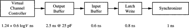
Now, these times are instantiated for every routing algorithm evaluated:
![]() Deterministic routing. This routing algorithm offers a single routing choice. The switch is usually made by cascading several low-size crossbars, one per dimension. Each of these crossbars switches messages going in the positive or negative direction of the same dimension or crossing to the next dimension. As there are two virtual channels per physical channel and two directions per dimension, the first crossbar in the cascade has eight ports, including four injection ports. Taking into account that dimensions are crossed in order, most messages will continue in the same dimension. Thus, the number of crossbars traversed will be one most of the times. So, for the deterministic routing algorithm, we have F = 1, P = 8, and V = 2, and we obtain the following delays for router, switch, and channel, respectively:
Deterministic routing. This routing algorithm offers a single routing choice. The switch is usually made by cascading several low-size crossbars, one per dimension. Each of these crossbars switches messages going in the positive or negative direction of the same dimension or crossing to the next dimension. As there are two virtual channels per physical channel and two directions per dimension, the first crossbar in the cascade has eight ports, including four injection ports. Taking into account that dimensions are crossed in order, most messages will continue in the same dimension. Thus, the number of crossbars traversed will be one most of the times. So, for the deterministic routing algorithm, we have F = 1, P = 8, and V = 2, and we obtain the following delays for router, switch, and channel, respectively:
![]() Partially adaptive routing. The number of routing choices is equal to two because there are two virtual channels per physical channel that can be used in most cases, but dimensions are crossed in order. Because dimensions are crossed in order, the switch can be the same as for the deterministic algorithm. Substituting F = 2, P = 8, and V = 2:
Partially adaptive routing. The number of routing choices is equal to two because there are two virtual channels per physical channel that can be used in most cases, but dimensions are crossed in order. Because dimensions are crossed in order, the switch can be the same as for the deterministic algorithm. Substituting F = 2, P = 8, and V = 2:
![]() Fully adaptive routing. In this case, the number of routing choices is five because we have one virtual channel in each dimension that can be used to cross the dimensions in any order, and also the two channels provided by the partially adaptive algorithm. As there are two channels per dimension, with three virtual channels per physical channel, plus four injection/delivery ports, the switch is a 22-port crossbar. Thus, we have F = 5, P = 22, and V = 3. Substituting we have
Fully adaptive routing. In this case, the number of routing choices is five because we have one virtual channel in each dimension that can be used to cross the dimensions in any order, and also the two channels provided by the partially adaptive algorithm. As there are two channels per dimension, with three virtual channels per physical channel, plus four injection/delivery ports, the switch is a 22-port crossbar. Thus, we have F = 5, P = 22, and V = 3. Substituting we have
Taking into account that all the delays for each routing algorithm are similar, the corresponding router can be implemented by performing each operation in one clock cycle. In this case, the clock period is determined by the slowest operation. Hence
The deterministic and the partially adaptive routing algorithms require the same clock period of 6.74 ns. Although routing delay is greater in the latter case, channel delay dominates in both cases and is therefore the bottleneck. For the adaptive algorithm, clock period increases up to 7.49 ns, slowing down clock frequency by 10% with respect to the other algorithms. It should be noted that clock frequency would be the same if a single injection/delivery port were used.
The following sections show the effect of router delays on performance. Note that plots in those sections are identical to the ones shown in Sections 9.4.1, 9.4.2, and 9.4.3, except that plots for each routing algorithm have been scaled by using the corresponding clock period. As the deterministic and the partially adaptive algorithms have the same clock frequency, comments will focus on the relative performance of the fully adaptive routing algorithm. Finally, note that as VLSI technology improves, channel propagation delay is becoming the only bottleneck. As a consequence the impact of router complexity on performance will decrease over time, therefore favoring the use of fully adaptive routers.
9.10.2 Performance under Uniform Traffic
Figure 9.34 shows the average message latency versus accepted traffic when using a uniform distribution for message destinations. Latency and traffic are measured in ns and flits/node/μs, respectively. Note that, in this case, accepted traffic has not been normalized because the normalizing factor is different for each routing algorithm.
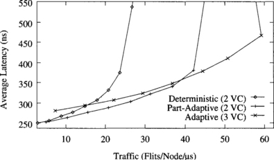
Figure 9.34 Average message latency versus accepted traffic for a uniform distribution of message destinations.
As expected, the lower clock frequency of the fully adaptive router produces a comparatively higher latency and lower throughput for the fully adaptive algorithm. Nevertheless, this algorithm still increases throughput by 103% and 28% with respect to the deterministic and the partially adaptive algorithms. However, for low loads, these algorithms achieve a latency up to 10% lower than the fully adaptive one. When the network is heavily loaded, the fully adaptive algorithm offers more routing options, achieving the lowest latency. Moreover, this algorithm also obtains a lower standard deviation of the latency (not shown) for the whole range of traffic.
9.10.3 Performance under Local Traffic
Figures 9.35 and 9.36 show the average message latency versus accepted traffic when message destinations are uniformly distributed inside a cube centered at the source node with each side equal to four and two channels, respectively.
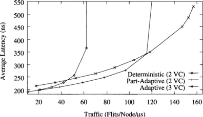
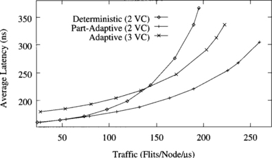
The relative behavior of the routing algorithms heavily depends on the average distance traveled by messages. When side = 4, the fully adaptive routing algorithm increases throughput by a factor of 2.5 with respect to the deterministic algorithm. However, the fully adaptive algorithm only achieves the lowest latency when the partially adaptive algorithm is close to saturation. Here, the negative effect of the lower clock frequency on performance can be clearly observed.
When traffic is very local, the partially adaptive algorithm achieves the highest throughput, also offering the lowest latency for the whole range of traffic. Nevertheless, it only improves throughput by 32% with respect to the deterministic algorithm. The fully adaptive algorithm exhibits the highest latency until accepted traffic reaches 60% of the maximum throughput. In this case, the negative effect of the lower clock frequency on performance is even more noticeable. As a consequence, adaptive routing is not useful when most messages are sent locally.
9.10.4 Performance under Nonuniform Traffic
Figures 9.37 and 9.38 show the average message latency versus accepted traffic for the bit reversal and the perfect shuffle traffic patterns, respectively.
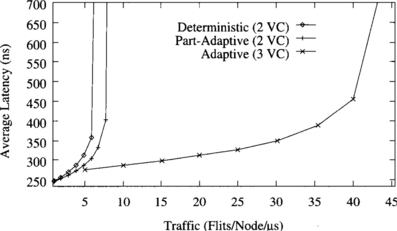
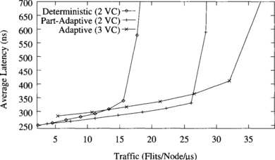
Figure 9.38 Average message latency versus accepted traffic for the perfect shuffle traffic pattern.
Despite the lower clock frequency, the fully adaptive algorithm increases throughput by a factor of 6.9 over the deterministic algorithm when the bit reversal communication pattern is used. For the perfect shuffle communication pattern, the fully adaptive algorithm doubles throughput with respect to the deterministic one. However, it only increases throughput by 35% over the partially adaptive algorithm. Also, this algorithm achieves a slightly lower latency than the fully adaptive one until it is close to the saturation point.
9.10.5 Effect of the Number of Virtual Channels
Section 9.7.1 showed that splitting physical channels into several virtual channels usually increases throughput but may increase latency when too many virtual channels are added. Also, it showed that virtual channels are more interesting for deterministic algorithms than for adaptive algorithms. In summary, the use of virtual channels has some advantages and some disadvantages. There is a trade-off.
In this section a more realistic analysis of the effect of adding virtual channels is presented. This study considers the additional propagation delay introduced by the circuits required to implement virtual channels. Note that increasing the number of virtual channels increases channel propagation delay. Moreover, it also increases the number of routing options and switch size, increasing routing delay and switch delay accordingly.
Assuming that all the operations are performed in a single clock cycle, Table 9.1 shows the clock period of the router as a function of the number of virtual channels per physical channel for the three routing algorithms under study. It has been computed according to the model presented in Section 9.10.1. For each value of the clock period, the slowest operation (tr, ts, or tw) is indicated.
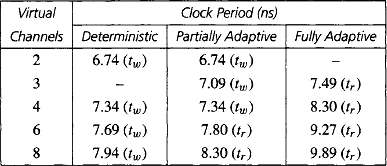
Figures 9.39, 9.40, and 9.41 show the effect of adding virtual channels to the deterministic, partially adaptive, and fully adaptive routing algorithms, respectively. Plots show the average message latency versus accepted traffic for a uniform distribution of message destinations.
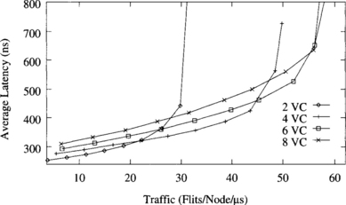
Figure 9.39 Average message latency versus accepted traffic as a function of the number of virtual channels for the deterministic routing algorithm.
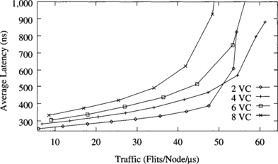
Figure 9.40 Average message latency versus accepted traffic as a function of the number of virtual channels for the partially adaptive routing algorithm.
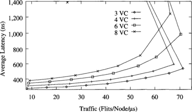
Figure 9.41 Average message latency versus accepted traffic as a function of the number of virtual channels for the fully adaptive routing algorithm.
For the deterministic algorithm there is a trade-off between latency and throughput. Adding virtual channels increases throughput, but it also increases latency. Therefore, depending on the requirements of the applications, the designer has to choose between achieving a lower latency or supporting a higher throughput. Anyway, changing from two to four virtual channels increases throughput by 52% at the expense of a small increment in the average latency. The standard deviation of latency is also reduced. The reason is that the additional channels allow messages to pass blocked messages. On the other hand, using eight or more virtual channels is not interesting at all because latency increases with no benefit.
However, adding virtual channels is not interesting at all for the partially adaptive and the fully adaptive routing algorithms. For the partially adaptive one, adding two virtual channels only increases throughput by 13%. Adding more virtual channels even decreases throughput. Moreover, the algorithm with the minimum number of virtual channels achieves the lowest latency except when the network is close to saturation. For the fully adaptive algorithm, adding virtual channels does not increase throughput at all.
Moreover, it increases latency significantly. Therefore, the minimum number of virtual channels should be used for both adaptive algorithms.
A similar study can be done for meshes. Although results are not shown, the conclusions are the same. For the deterministic routing algorithm, it is worth adding one virtual channel (for a total of two). Using three virtual channels increases throughput by a small amount, but it also increases latency. For the fully adaptive routing algorithm, using the minimum number of virtual channels (two channels) achieves the lowest latency. It is not worth adding more virtual channels.
9.11 Performance of Collective Communication
In this section, we present some evaluation results for networks implementing support for collective communication operations. Taking into account that communication start-up latency is very high in most multicomputers, we can expect a significant improvement in the performance of collective communication operations when some support for these operations is implemented in a parallel computer. However, the usefulness of implementing such support depends on how frequently collective communication operations are performed and on the number of nodes involved in each of those operations. So, depending on the applications running on the parallel computer, it may be useful or not to implement such support.
9.11.1 Comparison with Separate Addressing
Figure 9.42 compares the measured performance of separate addressing and a multicast tree algorithm (specifically, the spanning binomial tree presented in Section 5.5.2) for subcubes of different sizes on a 64-node nCUBE-2. The message length is fixed at 100 bytes. The tree approach offers substantial performance improvement over separate addressing.
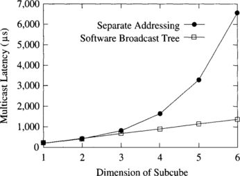
The U-mesh algorithm described in Section 5.7.4 was evaluated in [234]. The evaluation was performed on a 168-node Symult 2010 multicomputer, based on a 12 × 14 2-D mesh topology. A set of tests was conducted to compare the U-mesh algorithm with separate addressing and the Symult 2010 system-provided multidestination service Xmsend. In separate addressing, the source node sends an individual copy of the message to every destination. The Xmsend function was implemented to exploit whatever efficient hardware mechanisms may exist in a given system to accomplish multiple-destination sends. If there is no such mechanism, it is implemented as a library function that performs the necessary copying and multiple unicast calls.
Figure 9.43 plots the multicast latency values for implementations of the three methods. A large sample of destination sets was randomly chosen in these experiments. The message length was 200 bytes. The multicast latency with separate addressing increases linearly with the number of destinations. With the U-mesh algorithm, the latency increases logarithmically with the number of destinations. These experimental results demonstrate the superiority of the U-mesh multicast algorithm. Taking into account these results and that the U-mesh algorithm requires no hardware support, we can conclude that multicomputers should at least include a software implementation of multicast, regardless of how frequently this operation is performed.
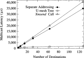
9.11.2 Comparing Tree-Based and Path-Based Algorithms
This section compares the performance of the double-channel XY multicast routing algorithm presented in Section 5.5.2, and the dual-path and multipath multicast algorithms presented in Section 5.5.3. These results were presented in [208]. The performance of a multicast routing algorithm depends not only on the delay and traffic resulting from a single multicast message, but also on the interaction of the multicast message with other network traffic. In order to study these effects on the performance of multicast routing algorithms, some simulations were run on an 8 × 8 mesh network. The simulation program modeled multicast communication in 2-D mesh networks. The destinations for each multicast message were uniformly distributed. All simulations were executed until the confidence interval was smaller than 5% of the mean, using 95% confidence intervals, which are not shown in the figures.
In order to compare the tree-based and path-based algorithms fairly, each algorithm was simulated on a network that contained double channels. Figure 9.44 gives the plot of average network latency for various network loads. The average number of destinations for a multicast is 10, and the message size is 128 bytes. The speed of each channel is 20 Mbytes/s. All three algorithms exhibit good performance at low loads. The path-based algorithms, however, are less sensitive to increased load than the tree-based algorithm. This result occurs because in tree-based routing, when one branch is blocked, the entire tree is blocked, increasing contention considerably. This type of dependency does not exist in path-based routing. Multipath routing exhibits lower latency than dual-path routing because, as shown above, paths tend to be shorter, generating less traffic. Hence, the network will not saturate as quickly. Although not shown in the figure, the variance of message latency using multipath routing was smaller than that of dual-path routing, indicating that the former is also generally more fair.
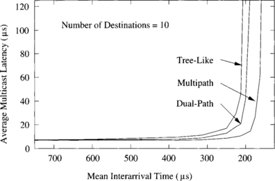
The disadvantage of tree-based routing increases with the number of destinations. Figure 9.45 compares the three algorithms, again using double channels. The average number of destinations is varied from 1 to 45. In this set of tests, every node generates multicast messages with an average time between messages of 300 μs. The other parameters are the same as for the previous figure.
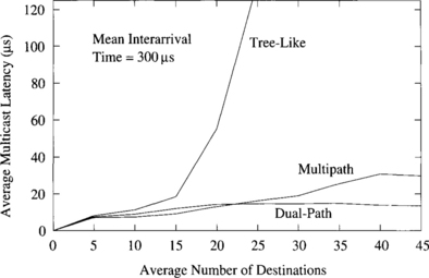
With larger sets of destinations, the dependencies among branches of the tree become more critical to performance and cause the delay to increase rapidly. The conclusion from Figures 9.44 and 9.45 is that tree-based routing is not particularly well suited for 2-D mesh networks when messages are relatively long. The path algorithms still perform well, however. Note that the dual-path algorithm results in lower latency than the multipath algorithm for large destination sets. The reason is somewhat subtle. When multipath routing is used to reach a relatively large set of destinations, the source node will likely send on all of its outgoing channels. Until this multicast transmission is complete, any flit from another multicast or unicast message that routes through that source node will be blocked at that point. In essence, the source node becomes a hot spot. In fact, every node currently sending a multicast message is likely to be a hot spot. If the load is very high, these hot spots may throttle system throughput and increase message latency. Hot spots are less likely to occur in dual-path routing, accounting for its stable behavior under high loads with large destination sets. Although all the outgoing channels at a node can be simultaneously busy, this can only result from two or more messages routing through that node.
Simulations were also run for multipath and dual-path routing with single channels and an average of 10 destinations. As the load increased, multipath routing offered slight improvement over dual-path routing. However, both routing algorithms saturated at a much lower load than with double channels (approximately for an average arrival time between messages of 350 μs), resulting in much lower performance than the tree-based algorithm with double channels. This result agrees with the performance evaluation presented in Section 9.4.1, which showed the advantage of using two virtual channels on 2-D meshes.
Finally, tree-based multicast with pruning (see Section 5.5.2) performs better than path-based multicast routing algorithms when messages are very short and the number of destinations is less than half the number of nodes in the network [224]. This makes tree-based multicast with pruning especially suitable for the implementation of cache-coherent protocols in distributed, shared-memory multiprocessors.
In summary, path-based multicast routing algorithms perform better than tree-based algorithms for long messages, especially for large destination sets. However, tree-based multicast performs better than path-based multicast when messages are very short. Finally, other design parameters like the number of virtual channels may have a stronger influence on performance than the choice of the multicast algorithm.
9.11.3 Performance of Base Routing Conformed Path Multicast
This section presents performance evaluation results for hardware-supported multicast operations based on the base routing conformed path (BRCP) model described in Section 5.5.3. For comparison purposes, the U-mesh and the Hamiltonian path-based routing algorithms are also evaluated. These results were presented in [268].
To verify the effectiveness of the BRCP model, single-source broadcasting and multicasting was simulated at the flit level. Two values for communication start-up time (ts) were used: 1 and 10 μs. Link propagation time (tp) was assumed to be 5 ns for a 200 Mbytes/s link. For unicast message passing, router delay (tnode) was assumed as 20 ns. For multidestination message passing a higher value of router delay, 40 ns, was considered. For a fair comparison, 2n consumption channels were assumed for both multidestination and unicast message passing, where n is the number of dimensions of the network. Each experiment was carried out 40 times to obtain average results.
Figures 9.46 and 9.47 compare the latency of single-source multicast on 2-D meshes for two network sizes and two ts values. Four different schemes were considered: a hierarchical leader-based (HL) scheme using (R, C) and (R, C, RC) paths, U-mesh, and a Hamiltonian path-based scheme. The simulation results show that the BRCP model is capable of reducing multicast latency as the number of destinations participating in the multicast increases beyond a certain number. This cutoff number was observed to be 16 and 32 nodes for the two network sizes considered.
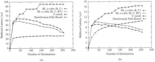
Figure 9.46 Comparison of single-source multicast latency on 16 × 16 meshes with two different communication start-up (ts) values: (a) ts = 10 μs and (b) ts = 1μs. (from [268])
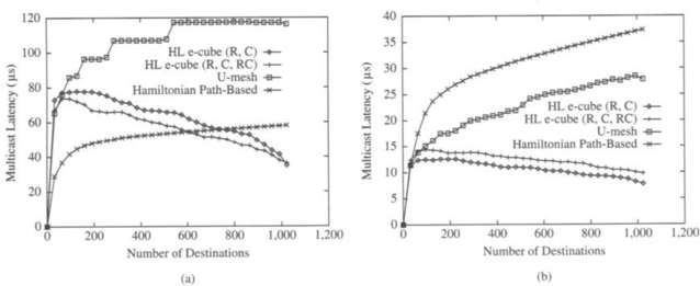
Figure 9.47 Comparison of single-source multicast latency on 32 × 32 meshes with two different communication start-up (ts) values: (a) ts = 10μs and (b) ts = 1μs. (from [268])
For a large number of destinations the HL schemes are able to reduce multicast latency by a factor of 2 to 3.5 compared to the U-mesh scheme. The Hamiltonian path-based scheme performs best for smaller system size, higher ts, and a smaller number of destinations per multicast. However, the HL schemes perform better than the Hamiltonian path-based scheme as the system size increases, ts reduces, and the number of destinations per multicast increases.
For systems with higher ts (10 μs), the HL scheme with RC paths was observed to implement multicast faster than using R and C paths. However, for systems with ts = 1 μs, the scheme using R and C paths performed better. This is because a multidestination worm along an RC path encounters longer propagation delay (up to 2k hops in a k × k network) compared to that along an R/C path (up to k hops). The propagation delay dominates for systems with lower ts. Thus, the HL scheme with R and C paths is better for systems with a lower ts value, whereas the RC path-based scheme is better for other systems.
9.11.4 Performance of Optimized Multicast Routing
This section evaluates the performance of several optimizations described in Chapter 5. In particular, the source-partitioned U-mesh (SPUmesh) algorithm, introduced in Section 5.7.4, and the source quadrant-based hierarchical leader (SQHL) and source-centered hierarchical leader (SCHL) schemes, described in Section 5.5.3, are compared to the U-mesh and hierarchical leader-based (HL) algorithms described in the same sections. The performance results presented in this section were reported in [173].
A flit-level simulator was used to model a 2-D mesh and evaluate the algorithms for multiple multicast. The parameters used were ts (communication start-up time) = 5 μs, tp (link propagation time) = 5 ns, tnode (router delay at node) = 20 ns, tsw (switching time across the router crossbar) = 5 ns, tinj (time to inject message into network) = 5 ns, and tcons (time to consume message from network) = 5 ns. The message length was assumed to be a constant 50 flits, and a 16 × 16 mesh was chosen. Each experiment was carried out 30 times to obtain average results. For each simulation, destination sets were randomly generated for each multicast message. In Figure 9.48(a), multicast latency is plotted against the number of sources (s), while keeping the number of destinations (d) fixed. In Figure 9.48(b), multicast latency is plotted against d, while keeping s fixed. The former shows the effect of the number of multicasts on latency, while the latter shows the effect of the size of the multicasts on latency.
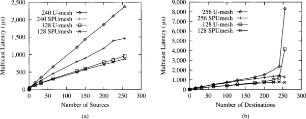
Figure 9.48 Multiple multicast latency on a 16 × 16 mesh using U-mesh and SPUmesh algorithms. Randomly generated destination sets with (a) fixed d (128, 240) with varying s and (b) fixed s (128, 256) with varying d. (from [173])
Figure 9.48(a) shows that the SPUmesh algorithm outperforms the U-mesh algorithm for large d by a factor of about 1.6. For small to moderate values of d, performance is similar. This is clear in Figure 9.48(b) where the U-mesh latency shoots up for larger d, whereas the SPUmesh latency remains more or less constant. The U-mesh algorithm behaves in this way because increasing d increases the number of start-ups the common center node will have to sequentialize. However, the SPUmesh algorithm performs equally well for both large and small d. This is because increasing d does not increase the node contention, as the multicast trees are perfectly staggered for identical destination sets.
It can be observed in Figure 9.49(a) that the SCHL scheme does about two to three times better than the SQHL scheme and about five to seven times better than the HL scheme. The HL scheme undergoes a large degree of node contention even for randomly chosen destinations. A property of the HL scheme observed in Section 9.11.3 is that latency reduces with increase in d. This basic property of the HL scheme is best exploited by the SCHL scheme. This can be noticed in Figure 9.49(b), where on increasing d the latency of SCHL drops. However, the SQHL scheme outperforms the SCHL scheme for small d, since the number of start-ups at the U-mesh stage of the multicast will be more for the SCHL scheme. There is a crossover point after which the SCHL scheme performs better. This can be seen Figure 9.49(b). The above results lead to the conclusion that node contention is one of the principal reasons for poor performance of existing multicast algorithms. Reducing node contention should be the primary focus while designing multicast algorithms.
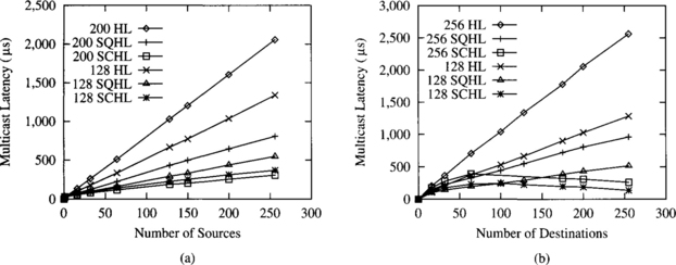
Figure 9.49 Multiple multicast latency on a 16 × 16 mesh using HL, SQHL, and SCHL schemes. Randomly generated destination sets with (a) fixed d (128, 200) with varying s and (b) fixed s (128, 256) with varying d. (from [173])
9.11.5 Performance of Unicast- and Multidestination-Based Schemes
This section compares multicast algorithms using unicast messages with those using multidestination messages. This measures the potential additional benefits that a system provides if it supports multidestination wormhole routing in hardware. The multicast algorithms selected for comparison are the ones that achieved the best performance in Section 9.11.4 (the SPUmesh and the SCHL schemes), using the same parameters as in that section. The performance results presented in this section were reported in [173].
As expected, the SCHL scheme outperforms the SPUmesh algorithm for both large and small d. This can be seen in Figure 9.50. Since the destination sets are completely random, there is no node contention to degrade the performance of the SCHL scheme. There is a crossover point at around d = 100, after which the SCHL scheme keeps improving as d increases. The reason is that hierarchical grouping of destinations gives relatively large leader sets for small d. This is because the destinations are randomly scattered in the mesh. On the other hand, SPUmesh generates perfectly staggered trees for identical destination sets. But, as d increases, leader sets become smaller and the advantage of efficient grouping in the SCHL scheme overcomes the node contention. This results in a factor of about 4−6 improvement over the SPUmesh algorithm when the number of sources and destinations is very high.
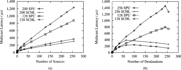
Figure 9.50 Multiple multicast latency on a 16 × 16 mesh using SPUmesh and SCHL. Randomly generated destination sets with (a) fixed d (128, 200) with varying s and (b) fixed s (128, 256) with varying d. (from [173])
These results lead to the conclusion that systems implementing multidestination message passing in hardware can support more efficient multicast than systems providing unicast message passing only. However, when the number of destinations for multicast messages is relatively small, the performance benefits of supporting multidestination message passing are small. So the additional cost and complexity of supporting multidestination message passing is only worth it if multicast messages represent an important fraction of network traffic and the average number of destinations for multicast messages is high.
9.11.6 Performance of Path-Based Barrier Synchronization
This section compares the performance of unicast-based barrier synchronization [355] and the barrier synchronization mechanism described in Section 5.6.2. These performance results were reported in [265].
A flit-level simulator was used to evaluate the algorithms for barrier synchronization. The following parameters were assumed: ts (communication start-up time) as 1 and 10 μs, tp (link propagation time) as 5 ns, and channel width as 32 bits. For multidestination gather and broadcast worms, bit string encoding was used. The node delay (tnode) was assumed to be 20 ns for unicast-based message passing. Although the node delay for multidestination worm (using bit manipulation logic) may be similar to that of unicast messages, three different values of node delay were simulated. In the simulation graphs, these values are indicated by 20 ns (1 × node delay), 30 ns (1.5 × node delay), and 40 ns (2 × node delay). The processors were assumed to be arriving at a barrier simultaneously. For arbitrary set barrier synchronization, the participating processors were chosen randomly. Each experiment was repeated 40 times, and the average synchronization latency was determined.
Complete Barrier
Complete barrier synchronization schemes were evaluated for the following 2-D mesh configurations with e-cube routing: 4 × 4, 8 × 4, 8 × 8, 16 × 8, 16 × 16, 32 × 16, 32 × 32, 64 × 32, and 64 × 64. Evaluations were done for ts = 1 μs and ts = 10 μs. Figure 9.51 shows the comparison. It can be observed that the multidestination scheme outperforms the unicast-based scheme for all system sizes. As the system size grows, the cost of synchronization increases very little for the multidestination scheme compared to the unicast-based scheme. The costs for 64 × 32 and 64 × 64 configurations are higher because the worm length increases by 1 flit to accommodate bit-encoded addresses with 32-bit channel width. With 1 μs communication start-up time, the multidestination scheme with 1 × node delay is able to barrier-synchronize 4K processors in just 11.68 μs. The unicast-based scheme also performs very well, being able to synchronize the same number of processors in 31 μs with no hardware support. For higher communication start-up, the cost with the multidestination scheme remains practically constant with increase in system size. This shows the effectiveness of the multidestination scheme to perform low-cost barrier synchronization in a large system in spite of higher communication start-up time.
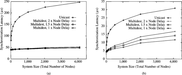
Figure 9.51 Comparison of unicast-based and multidestination-based schemes to implement complete barrier synchronization on 2-D meshes: (a) ts = 10μs and (b) ts = 1μs. (from [265])
Arbitrary Subset Barrier
The cost of arbitrary subset barrier synchronization was evaluated on 32 × 32 and 10 × 10 × 10 systems with different numbers of participating processors. A communication start-up time of 1 μs with varying node delays for the multidestination scheme was assumed. Figure 9.52 shows the comparison. It can be seen that as the number of participating processors increases beyond a certain number, the multidestination scheme is able to implement a barrier with reduced cost. This is the unique strength of this scheme. It shows the potential to implement dense barrier synchronization with reduced cost. Such crossover depends on system size, topology, communication start-up time, and node delay. For 1 × node delay, the crossover was observed at 96 nodes for the 32 × 32 system and 256 nodes for the 10 × 10 × 10 system. The crossover point is smaller for 2-D mesh compared to 3-D mesh. With a smaller number of processors participating in a barrier, the multidestination scheme performs a little worse due to longer paths traveled by multidestination worms. Beyond the crossover point, the multidestination scheme demonstrates steady reduction in cost over the unicast-based scheme. For 75% nodes participating in a barrier, with the technological parameters considered, the multidestination scheme reduces the synchronization cost by a factor of 1.4–2.7 compared to the unicast-based scheme. For higher communication start-up time and system size, the improvement will be higher.
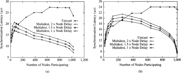
Figure 9.52 Comparison of unicast-based and multidestination-based schemes to implement arbitrary set barrier synchronization on (a) 2-D and (b) 3-D meshes. (from [265])
9.12 Software Messaging Layer
This section evaluates the overhead introduced by the software messaging layer. It also analyzes the impact of some optimizations.
9.12.1 Overhead of the Software Messaging Layer
The overhead of the software messaging layer and its contribution to the overall communication latency has been evaluated by several researchers on different parallel computers [85, 170, 171, 214, 354]. Here we present some recent performance evaluation results obtained by running benchmarks on an IBM SP2. These results have been reported in [238]. In the next section, we will show the drastic reduction in latency that can be achieved by establishing virtual circuits between nodes before data are available and by reusing those circuits for all the messages exchanged between those nodes.
The SP2 communication subsystem is composed of the high-performance switch plus the adapters that connect the nodes to the switch [5, 329, 330]. The adapter contains an onboard microprocessor to off-load some of the work of passing messages from node to node and some memory to provide buffer space. DMA engines are used to move information from the node to the memory of the adapter and from there to the switch link.
Three different configurations of the communication subsystem of the IBM SP2 were evaluated. In the first configuration, the adapters were based on an Intel i860, providing a peak bandwidth of 80 Mbytes/s. The links connecting to the high-performance switch provided 40 Mbytes/s peak bandwidth in each direction, with a node-to-node latency of 0.5 μs for systems with up to 80 nodes. The operating system was AIX version 3, which included MPL, a proprietary message-passing library [324]. An implementation of the MPI interface [44] was available as a software layer over MPL. In the second configuration, the communication hardware was identical to the first configuration. However, the operating system was replaced by AIX version 4, which includes an optimized implementation of MPI. In the third configuration, the network hardware was updated, keeping AIX version 4. The new adapters are based on a PowerPC 601, achieving a peak transfer bandwidth of 160 Mbytes/s. The new switch offers 300 Mbytes/s peak bidirectional bandwidth, with latencies lower than 1.2 μs for systems with up to 80 nodes.
The performance of point-to-point communication was measured using the code provided in [85] for systems using MPI. The performance of the IBM SP2 is shown in Table 9.2 for the three configurations described above and different message lengths (L). The words “old” and “new” refer to the communications hardware, and “v3” and “v4” indicate the version of the operating system. As can be seen, software overhead dominates communication latency for very short messages. Minimum latency ranges from 40 to 60 μs while hardware latency is on the order of 1 μs. As a consequence, software optimization has a stronger effect on reducing latency for short messages than improving network hardware. This is the case for messages shorter than 4 Kbytes. However, for messages longer than 4 Kbytes the new version of the operating system performs worse. The reason is that for messages shorter than 4 Kbytes an eager protocol is used, sending messages immediately, while for longer messages a rendezvous protocol is used, sending a message only when the receiver node agrees to receive it. Switching to the rendezvous protocol incurs higher start-up costs but reduces the number of times information is copied when using the new hardware, thus reducing the cost per byte for the third configuration. Finally, the higher peak bandwidth of the new hardware can be clearly appreciated for messages longer than 10 Kbytes.
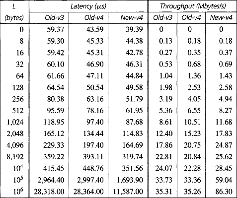
An interesting observation is that the message length required to achieve half the maximum throughput is approximately 3 Kbytes for the old hardware configuration and around 32 Kbytes for the new network hardware. Thus, improving network bandwidth without reducing software overhead makes it even more difficult to take advantage of the higher network performance. Therefore, the true benefits of improving network hardware will depend on the average message size.
Several parallel kernels have been executed on an IBM SP2 with 16 Thin2 nodes. These kernels include four benchmarks (MG, LU, SP, and BT) from the NAS Parallel Benchmarks (NPB) version 2 [14] and a shallow water modeling code (SWM) from the ParkBench suite of benchmarks [350]. Only the first and third configurations described above for the communication subsystem were evaluated (referred to as “old” and “new”, respectively).
Figure 9.53 shows the execution time in seconds and the average computation power achieved for the different benchmarks. It can be clearly seen that the performance of all the applications is almost the same for the old and new configurations because average message lengths are shorter than 10 Kbytes.
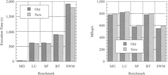
Figure 9.53 Execution time and average computation power achieved for the different benchmarks on an IBM SP2 with 16 Thin2 nodes. (from [238])
Therefore, software overhead has a major impact on the performance of parallel computers using message-passing libraries. Improving network hardware will have an almost negligible impact on performance unless the latency of the messaging layer is considerably reduced.
9.12.2 Optimizations in the Software Messaging Layer
In this section we present some performance evaluation results showing the advantages of establishing virtual circuits between nodes, and caching and reusing those circuits. This technique is referred to as virtual circuit caching (VCC). VCC is implemented by allocating buffers for message transmission at source and destination nodes before data are available. Those buffers are reused for all the subsequent transmissions between the same nodes, therefore reducing software overhead considerably. A directory of cached virtual circuits is kept at each node. The evaluation results presented in this section are based on [81].
The simulation study has been performed using a time-step simulator written in C. The simulated topology is a k-ary n-cube. A simulator cycle is normalized to the time to transmit one flit across a physical link. In addition, the size of one flit is 2 bytes. Since the VCC mechanism exploits communication locality, performance evaluation was performed using traces of parallel programs. Traces were gathered for several parallel kernels executing on a 256-processor system.
The communication traces were collected using an execution-driven simulator from the SPASM toolset [323]. The parallel kernels are the (1) broadcast-and-roll parallel matrix multiply (MM), (2) a NAS kernel (EP), (3) a fast Fourier transform (FFT), (4) a Kalman filter (Kalman), and (5) a multigrid solver for computing a 3-D field (MG). The algorithm kernels display different communication traffic patterns.
Locality Metrics
The following metric attempts to capture communication locality by computing the average number of messages that are transmitted between a pair of processors:
This metric gives a measure of the number of messages that can use the same circuit, which as a result may be worth caching. However, this measure does not incorporate any sense of time; that is, there is no information about when each of the individual messages are actually sent relative to each other. In analyzing a trace for communication locality, we can compute the expression above over smaller intervals of time and produce a value that would be the average message density per unit of time. If parallel algorithms are structured to incorporate some temporal locality (i.e., messages from one processor to another tend to be clustered in time), then this measure will reflect communication locality. A trace with a high value of message density is expected to benefit from the use of the cacheable channels. Table 9.3 shows the computed values of the average message density for the traces under study. The traces with a value of 0.0 (EP, FFT, MG) possess no locality. They have no (source, destination) pairs that send more than one message to each other. The other traces have nonzero values, implying that reuse of circuits is beneficial.
The Effects of Locality
An uncached message transmission was modeled as the sum of the messaging layer overhead (including the path setup time) and the time to transmit a message. The overhead includes both the actual system software overhead and the network interface overhead. For example, this overhead was measured on an Intel Paragon, giving an approximate value of 2,600 simulator cycles. However, the selected value for the overhead was 100 simulator cycles, corresponding to the approximate reported measured times for Active Message implementations [105]. A cached message transmission is modeled as the sum of the time to transmit the message (the actual data transmission time) and a small overhead to model the time spent in moving the message from user space to the network interface and from the network interface back into the user space. In addition, there is overhead associated with each call to set up a virtual circuit. This overhead is equivalent to that of an uncached transmission. There is also overhead associated with the execution of the directive to release a virtual circuit.
The effect of VCC is shown in Table 9.4. The differences are rather substantial, but there are several caveats with respect to these results. The VCC latencies do not include the amortized software overhead, but rather only network latencies. The reason is the following. The full software overhead (approximately 100 cycles) is only experienced by the first message to a processor. Subsequent messages experience the latencies shown in Table 9.4. Moreover, if virtual circuits are established before they are needed, it is possible to overlap path setup with computation. In this case, the VCC latencies shown in Table 9.4 are the latencies actually experienced by messages. Since these traces were simulated and optimized by manual insertion of directives in the trace, almost complete overlap was possible due to the predictable nature of many references. It is not clear that automated compiler techniques could do nearly as well, and the values should be viewed in that light. The VCC entries in the table are the average experienced latencies without including path setup time. The non-VCC latencies show the effect of experiencing overhead with every transmission. Although EP, FFT, and MG do not exhibit a great degree of locality, the results exhibit the benefit of overlapping path setup with computation. Finally, the overhead of 100 cycles is only representative of what is being reported these days with the Active Message [105] and the Fast Message [264] implementations. Anyway, the latency reduction achieved by using VCC in multicomputers is higher than the reduction achieved by other techniques.
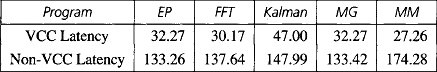
9.13 Performance of Fault-Tolerant Algorithms
In this section, we present evaluation results for several fault-tolerant routing protocols. This evaluation study analyzes the performance of the network in the presence of faults using synthetic workloads. Also, the probability of completion for some parallel kernels in the presence of faults is studied. A wide range of solutions to increase fault tolerance has been considered, covering a spectrum from software-based fault-tolerant routing protocols to very resilient protocols based on PCS. Although some of these results have been published recently [79, 126, 333], other results are entirely new.
9.13.1 Software-Based Fault-Tolerant Routing
In this section we evaluate the performance of the software-based fault-tolerant routing protocols presented in Section 6.5.2. These techniques can be used on top of any deadlock-free routing algorithm, including oblivious e-cube routing and fully adaptive Duato’s protocol (DP). The resulting fault-tolerant routing protocols are referred to as e-sft and DP-sft, respectively.
The performance of e-sft and DP-sft was evaluated with flit-level simulation studies of message passing in a 16-ary 2-cube with 16-flit messages, a single-flit routing header, and eight virtual channels per physical channel. Message destination traffic was uniformly distributed. Simulation runs were made repeatedly until the 95% confidence intervals for the sample means were acceptable (less than 5% of the mean values). The simulation model was validated using deterministic communication patterns. We use a congestion control mechanism (similar to [36]) by placing a limit on the size of the buffer on the injection channels. If the input buffers are filled, messages cannot be injected into the network until a message in the buffer has been routed. Injection rates are normalized.
Cost of e-sft and DP-sft
The header format for e-sft and DP-sft was presented in Figure 6.29. A 32-bit header enables routing within a 64 × 64 torus. The flags require 6 bits, and the offsets require 6 bits each.
We assume the use of half-duplex channels. With half-duplex channels, 32-bit channels are comparable to the number of data pins devoted to interrouter communication in modern machines (e.g., there are two 16-bit full-duplex channels in the Intel Paragon router). A flit crosses a channel in a single cycle and traverses a router from input to output in a single cycle. Use of 16-bit full-duplex channels would double the number of cycles to transmit the routing header. Routing decisions are assumed to take a single cycle with the network operating with a 50 MHz clock and 20 ns cycle time. The software cost for absorbing and reinjecting a message is derived from measured times on an Intel Paragon and reported work with Active Message implementations [105]. Based on these studies, we assess this cost nominally at 25 μs per absorption/injection or 50 μs each time a message must be processed by the messaging software at an intermediate node. If the message encounters busy injection buffers when it is being reinjected, it is requeued for reinjection at a later time. Absorbed messages have priority over new messages to prevent starvation.
The router hardware can retain the same basic architecture as the canonical form for dimension-order routers or adaptive routers presented in Section 7.2.1, which captures the basic organization of several commercial and research designs. The only additional functionality required is of the routing and arbitration unit. When a message is routed to a faulty output channel, the F bit must be set and the X-Dest and Y-Dest fields reset to 0 to cause the message to be absorbed. One side effect of the increased header size is a possible increase in virtual channel buffer size and the width of the internal data paths, although 32-bit data paths appear to be reasonable for the next generation of routers. Finally, as with any approach for fault-tolerant routing, support for testing of channels and nodes must be available. The remaining required functionality of e-sft and DP-sft is implemented in the messaging layer software.
Simulation Results
In a fault-free network the behavior of e-cube and e-sft is identical, with slightly lower performance for e-sft due to the larger header size. Simulation experiments placed a single fault region within the network. The performances of e-sft and DP-sft are shown in Figure 9.54 for a 9-node convex fault region and for an 11-node concave fault region. Due to the greater difficulty in entering and exiting a concave fault region, the average message latency is substantially greater in the presence of concave fault regions than for equivalent-sized convex fault regions. The message latency for DP-sft is significantly lower than the message latency for e-sft. The reason is that when a fault is encountered, DP-sft is able to find an alternative fault-free path in most cases. However, the only choice for e-sft is absorbing the message. The curves also indicate that for each of the fault configurations the latency remains relatively constant as the accepted traffic increases. As network load increases, the number of messages each node injects and receives increases, but the percentage of messages that encounter the fault region remains relatively constant. Therefore, the latency remains relatively flat. Another factor is that the high latencies of rerouted messages mask some of the growth in the latency of messages that do not encounter faults, although a close inspection of the graphs reveals a small but steady growth in average latency. For the concave fault region and DP-sft, this growth rate is larger because, with adaptive routing, the number of messages that encounter a fault increases with load. The high latencies of these messages contribute to the faster growth in average message latency.
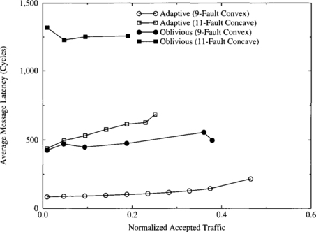
Figure 9.54 Average message latency versus normalized accepted traffic for e-sft and DP-sft with a 9-node convex fault block and an 11-node concave fault block.
Figure 9.55 shows the performances of e-sft and DP-sft in the presence of a single convex fault region ranging in size from 1 to 21 failed nodes. For each plot the message injection rate (normalized applied load) is indicated in parentheses. The latency plots indicate that when the network is below saturation traffic the increase in the size of the fault block causes significant increases in the average message latency for e-sft. This is due to the increase in the number of messages encountering fault regions (a 1-node fault region represents 0.4% of the total number of nodes in the network, while a 21-node fault region represents 8.2% of the total number of nodes). But in DP-sft the average message latencies remain relatively constant since at low loads a larger percentage of messages (relative to e-sft) can be routed around the fault regions and can avoid being absorbed. The latency and accepted traffic curves for a high injection rate (0.576) represent an interesting case. Latency and accepted traffic for e-sft appear to remain relatively constant. At high injection rates and larger fault regions, more messages become absorbed and rerouted. However, the limited buffer size provides a natural throttling mechanism for new messages as well as absorbed messages waiting to be reinjected. As a result, active faulted messages in the network form a smaller percentage of the traffic, and both the latency and accepted traffic characteristics are dominated by the steady-state values of traffic unaffected by faults. The initial drop in accepted traffic for a small number of faults is due to the fact that initially a higher percentage of faulted messages is delivered, reducing accepted traffic. These results suggest that sufficient buffering of faulted messages and priorities in reinjecting them have a significant impact on the performance of faulted messages. However, for a high injection rate (0.576) and DP-sft, the average message latency increases and the accepted traffic decreases as the number of faults is increased. At high injection rates congestion increases. Messages encountering a fault may also find that all the alternative paths offered by DP-sft are busy. Because messages are not allowed to block if the channel used to escape from deadlock is faulty, those messages are absorbed. Thus, the percentage of messages that are absorbed after encountering a fault increases with applied load, therefore increasing latency and reducing accepted traffic. At low injection rates, the accepted traffic remains relatively constant independent of the size of the fault blocks since fault blocks only increase the latency of the messages. Note that for lower injection rates the accepted traffic curves for e-sft and DP-sft are identical. Since messages are guaranteed delivery when operating well below saturation, the network quickly reaches the steady state for accepted traffic.
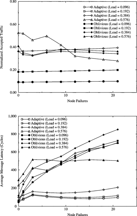
Figure 9.55 Normalized accepted traffic and average message latency as a function of node failures (convex regions).
The plots in Figure 9.56 show the number of messages queued by message-absorbing nodes for message injection rates (normalized applied load) of 0.096, 0.192, 0.384, and 0.576, in the presence of a single convex fault region ranging in size from 1 to 21 failed nodes. This is simply a count of the number of messages absorbed due to faults. A given message contributes more than once to this count if it is absorbed multiple times. As expected, the number of messages queued increases as the number of node faults increases. Also, the number of messages queued is much higher for e-sft than for DP-sft. At lower injection rates the number of messages absorbed increases rather slowly, remaining relatively constant for DP-sft while approximately doubling for e-sft. This number increases rapidly for higher injection rates. At an injection rate of 0.576, the rate of increase decreases as the number of faults increases for e-sft. Note that DP-sft displays contrasting behavior. Eventually, the number of absorbed messages is limited by the buffering capacity for faulted messages. This limit is reached by e-sft much earlier than by DP-sft. Figure 9.57 shows similar behavior in the presence of convex and concave regions; that is, on the average, concave regions cause more messages to be absorbed.

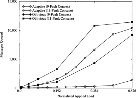
In general, the number of times a message is rerouted is relatively small. In practice, the probability of multiple router failures before repair is very low in most systems. In these systems, the large majority of faulted messages will not have to pass through more than one node. This makes these techniques attractive for next-generation wormhole-routed networks. In summary, it can be observed that the performance of rerouted messages is significantly affected by techniques for buffering and reinjection. At low to moderate loads, the performance of adaptive routing protocols provides substantial performance improvements over oblivious protocols. At high fault rates and loads beyond saturation, increased adaptivity can cause severe performance degradation due to increased congestion. At high loads and high fault rates, oblivious protocols are limited by buffering capacity while adaptive protocols are limited by congestion.
9.13.2 Routing Algorithms for PCS
This section evaluates the performance of two backtracking protocols using pipelined circuit switching (PCS) and compares them with three routing protocols using wormhole switching. Performance is analyzed both in fault-free networks and in the presence of static faults. The backtracking protocols analyzed in this section are exhaustive profitable backtracking (EPB) and misrouting backtracking with m misroutes (MB-m). These protocols were described in Section 4.7. The wormhole protocols analyzed here are Duato’s protocol (DP), dimension reversal routing (DR), and negative-first (NF). These protocols were described in Sections 4.4.4 and 4.3.2.
Given a source/destination pair (s, d), let si, di be the ith dimension coordinates for s and d, respectively. Let |si − di|k denote the torus dimension distance from si to di defined by
We performed simulation studies on 16-ary 2-cubes to evaluate the performance of each protocol. Experiments were conducted with and without static physical link faults under a variety of network loads and message sizes. For all routing protocols except NF, a processor s was allowed to communicate to other processors in the subcube defined by {d : |si − di|k ≤ 4, i = 1, …, n}. This corresponds to a neighborhood of about one-half the network diameter. Destinations were picked uniformly through this neighborhood. Since NF is not allowed to use end-around connections, the communication neighborhood was defined by {d : |si − di| ≤ 4, i − 1, …, n}. Thus, the diameter of the communication patterns was comparable for all routing protocols. A simulator cycle was normalized to the time to transmit one flit across a physical link. Each simulation was run for 30,000 global clock cycles, discarding information occurring during a 10,000-clock-cycle warm-up period. The transient start-up period was determined by monitoring variations in the values of performance parameters. We noted that after a duration of 10,000 network cycles, the computed parameter values did not deviate more than 2%. The recorded values in the start-up interval were discarded. In a moderately loaded network, in the 20,000 clock cycles over which statistics were gathered, over 800,000 flits were moved through the network. Each simulation was run repeatedly to obtain a sample mean and a sample variance for each measured value. Runs were repeated until the confidence intervals for the sample means were acceptable. The simulation model was validated using deterministic communication patterns. Simulations on single messages in traffic-free networks gave the theoretical latencies and setup times for wormhole and PCS messages. In addition, tests were performed on individual links to ensure that the simulated mechanisms for link arbitration in the presence of multiple virtual circuits over the link functioned correctly.
Fault-Free Performance
In this study we performed experiments on fault-free 16-ary 2-cubes. Each physical link multiplexed 16 virtual channels in each direction. We ran the simulations for message sizes of 16 and 256 flits. The primary purpose of this study was to show the relative performance of PCS and wormhole switching under fault-free conditions. Figure 9.58 shows average latency versus normalized accepted traffic for the protocols under study. Latency is measured in clock cycles. If we assume normal distributions, the 95% confidence intervals for the normalized accepted traffic and latency data points were all within 5% of their values.
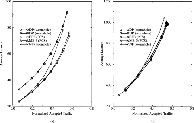
We see from the graphs that the added overhead of PCS causes a significant performance penalty over wormhole switching at lower message sizes. This penalty grows with the average number of links in the communication path. It is also interesting to note that the penalty appears to be relatively flat across the range of network loads. The relative network throughput capacity is not significantly reduced by the use of PCS. And, as message sizes get large, PCS’s performance approaches that of wormhole switching since the overhead is a much smaller fraction of the total communication latency. A similar set of experiments was performed using uniformly distributed destination addresses. The overall trends were identical to those found in Figure 9.58. Since the average path length is larger in the uniformly distributed message pattern, the performance penalty for PCS was proportionately larger.
Fault-Tolerant Performance
In this study we performed experiments on 16-ary 2-cubes with faulty physical links. We use physical link faults to address the performance of the protocols under changes in network topology. We are primarily concerned with overall network throughput (measured by accepted traffic) rather than delivery of individual messages and therefore focus on the effect of failures causing a change in network topology. Figures 9.59 and 9.60 show the normalized accepted traffic of each protocol as physical link faults in the system increase for a moderate network load. The network load is defined by establishing a desired normalized injection rate λi. We chose λi ≈ 0.26 since that is close to half of the normalized network throughput capacity (from Figure 9.58 we see that normalized network throughput appears to lie between 0.5 and 0.6). The four graphs correspond to networks with 1, 4, 8, and 16 virtual channels per physical link direction, respectively. Assuming the measured accepted traffic is normally distributed, the 95% confidence intervals for each point on the graph are indicated by the error bars.
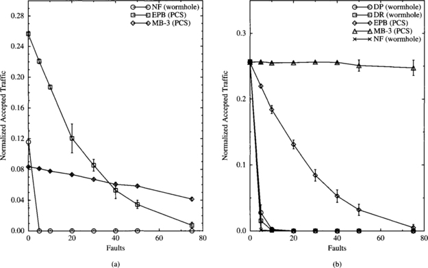
Figure 9.59 Normalized accepted traffic versus network faults: (a) L = 16, v = 1; (b) L = 16, v = 4.
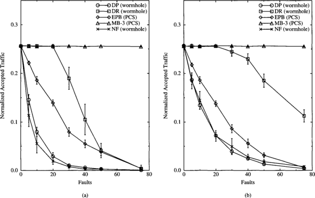
Figure 9.60 Normalized accepted traffic versus network faults: (a) L = 16, v = 8; (b) L = 16, v = 16.
In networks with only one virtual channel per physical link direction, only NF, EPB, and MB-3 were studied since DP and DR require multiple virtual channels per physical link. In the graph with v = 1, we see that the cost of misrouting in networks without multiple virtual channels is very high. The realizable network throughput for NF was less than half of the desired injection rate. For MB-3 it was only a third of λi. Despite its poor throughput, MB-3 displays good relative performance as the number of faulty links in the network increases. The sustainable throughput for NF with v = 1 is 0 for five or more physical link faults in the network. The realizable network throughput for EPB declines steadily as faults are introduced into the network.
For v = 4, the picture changes considerably. Using multiple virtual channels significantly reduces the cost and likelihood of misrouting. The misrouting protocols NF, MB-3, and DR can all sustain the desired injection rate in networks with no faulty links. With five faulty physical links, however, all of the progressive (wormhole) protocols display extremely reduced throughput. With 10 or more faulty physical links, the wormhole protocols are frequently deadlocked. MB-3 demonstrates a very flat normalized accepted traffic for up to 75 failed physical links (14.65% of the physical links).
As the number of virtual channels grows even higher, we see that the wormhole protocols develop more resilience to faults. With v = 8, DR is able to sustain the desired network throughput for up to 20 link failures. NF and DP show marginal improvement. DP suffers due to the fact that it is unable to misroute. Thus, any failed link will disconnect some portion of the network. Eventually, a message will stall on a faulty link and cause deadlock. Similarly NF suffers from the fact that misrouting is disabled after the first positive-going link is used. With v = 16, DR, NF, and DP show further marginal improvement. Recent studies have shown that the implementation and performance costs of using virtual channels can be significant [57]. Such results favor the use of protocols that work well with smaller numbers of virtual channels.
Overall, we can make the following observations:
1. As a rule, protocols that have great freedom in misrouting (DR, MB-3) tolerate faults better than those with limited or no misrouting (NF, DP, EPB).
2. MB-3 provides the best overall fault-tolerant performance.
3. The progressive protocols for wormhole switching benefit from increased numbers of virtual channels, while the fault-tolerant performance of backtracking PCS protocols is relatively insensitive to the number of virtual channels.
4. DR needs many virtual channels to provide higher levels of fault-tolerant behavior.
5. For fine-grained message passing, the performance of PCS protocols relative to wormhole switching drops off rapidly, and the primary benefit is better fault tolerance properties. For larger ratios of message sizes to message distance, performance approaches that of wormhole switching.
9.13.3 Routing Algorithms for Scouting
In this section we evaluate the performance of the two-phase (TP) routing protocol described in Section 6.6. When no faults are present in the network, TP routing uses K = 0 and the same routing restrictions as DP. This results in performance that is identical to that of DP. To measure the fault tolerance of TP, it is compared with misrouting backtracking with m misroutes (MB-m).
Fault-Tolerant Performance
The performance of the fault-tolerant protocols was evaluated with simulation studies of message passing in a 16-ary 2-cube with 32-flit messages. The routing header was one flit long. The message destination traffic was uniformly distributed. Simulation runs were made repeatedly until the 95% confidence intervals for the sample means were acceptable (less than 5% of the mean values). The simulation model was validated using deterministic communication patterns. We use a congestion control mechanism (similar to [36]) by placing a limit on the size of the buffer (eight buffers per injection channel) on the injection channels. If the input buffers are filled, messages cannot be injected into the network until a message in the buffer has been routed. A flit crosses a link in one cycle. The metrics used to measure the performance of TP are average message latency and accepted traffic.
The fault performance of TP is evaluated with a configuration of TP that uses K = 0 in fault-free segments. It also uses K = 0 in the faulty regions, that is, it does not use unsafe channels, and then it uses misrouting backtracking search to construct detours when the header cannot advance.
Figure 9.61 is a plot of the latency-traffic curves of TP and MB-m with 1, 10, and 20 failed nodes randomly placed throughout the network. The performance of both routing protocols drops as the number of failed nodes increases, since the number of undeliverable messages increases as the number of faults increases. MB-m degrades gracefully with steady but small drops in the network throughput as the number of faults increases. However, the latency of TP-routed messages for a given network load remains 30–40% lower than that of MB-m routed messages.
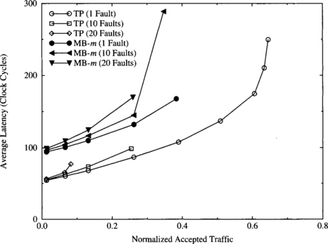
Figure 9.62 shows the normalized accepted traffic and average latency of TP and MB-m as a function of node failures under varying applied loads. This figure shows that the latency of messages successfully routed via MB-m remains relatively flat regardless of the number of faults in the system. The number in parentheses indicates the normalized applied load. However, with the normalized applied load at 0.384, the latency increased considerably as the number of faults increased. This is because with a low number of faults in the system, an applied load of 0.384 is at the saturation point of the network. With the congestion control mechanism provided in the simulator, any additional applied load is not accepted. However, at the saturation point, any increase in the number of faults will cause the aggregate bandwidth of the network to increase beyond saturation and therefore cause the message latency to increase and the network throughput to drop. When the applied load was at 0.64, the network was already beyond saturation so the increase in the number of faults had a lesser effect.
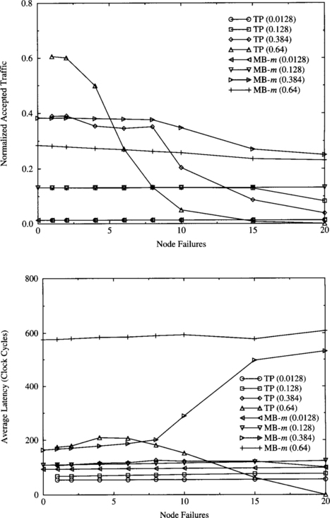
Figure 9.62 Normalized accepted traffic and average message latency of TP and MB-m as a function of node faults.
At low to moderate loads, and even at high loads with a low number of faults, the latency and accepted traffic characteristics of TP are significantly superior to that of MB-m. The majority of the benefit is derived from messages in fault-free segments of the network transmitting with K = 0 (i.e., wormhole switching). TP, however, performed poorly at high loads as the number of faults increased. While saturation traffic with 1 failed node was 0.64, it dropped to slightly over 0 with 20 failed nodes. It should be noted that in the simulated system (a 16-ary 2-cube), 20 failed nodes surpass the limit for which TP was designed. Anyway, the performance of TP with a high number of faults is very good as long as the applied load is low to moderate. At higher loads and an increased number of faults, the effect of the positive acknowledgments due to the detour construction becomes magnified and performance begins to drop. This is due to the increased number of searches that the routing header has to perform before a path is successfully established and the corresponding increase in the distance from the source node to the destination. The trade-off in this version of TP is the increased number of detours constructed versus the performance of messages in fault-free sections of the network. With larger numbers of faults, the former eventually dominates. In this region, purely conservative protocols like MB-m appear to work better.
In summary, at low fault rates and below network saturation loads, TP performs better than MB-m. We also note that the TP protocol used in the experiments was designed for three faults (2n − 1 in a 2-D network). A relatively more conservative version could have been configured. Figure 9.63 compares the performance of TP with K = 0 and K = 3. With only one fault in the network and low network traffic, both versions realize similar performance. However, with high network traffic and a larger number of faults, the aggressive TP performs considerably better. This is due to the fact that with K > 0, substantial acknowledgment flit traffic can be introduced into the network, dominating the effect of an increased number of detours.
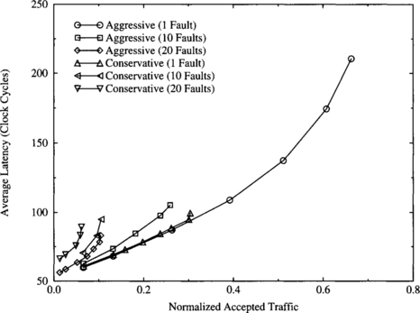
Cost of Supporting Dynamic Faults
When dynamic faults occur, messages may become interrupted. In Section 6.7 a special type of control flit, called a release flit, was introduced to permit distributed recovery in the presence of dynamic faults.
These control flits release any reserved buffers, notify the source that the message was not delivered, and notify the destination to ignore the message currently being received. If we are also interested in guaranteeing message delivery in the presence of dynamic faults, the complete path must be held until the last flit is delivered to the destination. A message acknowledgment sent from the destination removes the path and flushes the copy of the message at the source. Here we are only interested in the impact on the performance of TP. Figure 9.64 illustrates the overhead of this recovery and reliable message delivery mechanism.
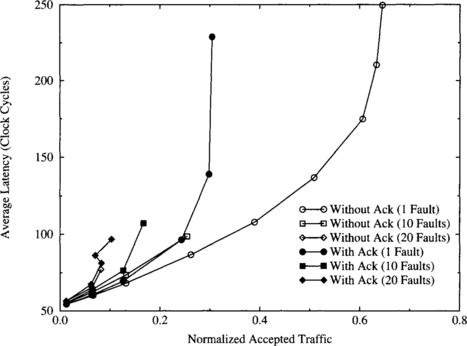
The additional message acknowledgment introduces additional control flit traffic into the system. Message acknowledgments tend to have a throttling effect on the injection of new messages. As a result, TP routing using the mechanism saturates at lower network loads, and delivered messages have higher latencies. From the simulation results shown in Figure 9.64, we see that at low loads the performance impact of support for dynamic fault recovery is not very significant. However, as applied load increases, the additional traffic generated by the recovery mechanism and the use of message acknowledgments begins to produce a substantial impact on performance. The point of interest here is that dynamic fault recovery has a useful range of feasible operating loads for TP protocols. In fact, this range extends almost to saturation traffic.
Trace-Driven Simulation
The true measure of the performance of an interconnection network is how well it performs under real communication patterns generated by actual applications. The network is considered to have failed if the program is prevented from completing due to undeliverable messages. Communication traces were derived from two different application programs: EP (Gaussian Deviates) and MMP (Matrix Multiply). These program traces were generated using the SPASM execution-driven simulator [323].
Communication-trace-driven simulations were performed allowing only physical link failures. Node failures would require the remapping of the processes, with the resulting remapping affecting performance. No recovery mechanisms were used for recovery of undeliverable messages. The traces were generated from applications executing on a 16-ary 2-cube. The simulated network was a 16-ary 2-cube with 8 and 16 virtual channels per physical link. The aggressive version of TP was used; that is, no unsafe channels were used. Figure 9.65 shows plots of the probability of completion for the two different program traces with differing values of misrouting (m). A trace is said to have completed when all trace messages have been delivered. If even one message cannot be delivered, program execution cannot complete. The results show the effect of not having recovery mechanisms. These simulations were implemented with no retries attempted when a message backtracks to the source or the node containing the first data flit. This is responsible for probabilities of completion below 1.0 for even a small number of faults. The performance effects of the recovery mechanism were illustrated in Figure 9.64. We expect that two or three retries will be sufficient in practice to maintain completion probabilities of 1.0 for a larger number of faults.
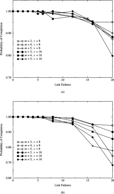
Figure 9.65 Probability of completion for various program traces and numbers of allowed misroutes: (a) EP and (b) MMP.
In some instances, an increased number of misroutes resulted in poorer completion rates. We believe that this is primarily due to the lack of recovery mechanisms and retries. Increased misrouting causes more network resources to be reserved by a message. This may in turn increase the probability that other messages will be forced to backtrack due to busy resources. Without retries, completion rates suffer. Again we see the importance of implementing relatively simple heuristics such as a small number of retries. Finally, the larger number of virtual channels offered better performance since it provided an increase of network resources and hence reduced the amount of searching required by routing headers.
Specifically, the performance evaluation provided the following insights:
1. The cost of positive acknowledgments in TP dominates the cost of detour construction, suggesting the use of low values of K, preferably K = 0.
2. Configurable flow control enables substantial performance improvement over PCS for a low to modest number of faults since the majority of traffic is in the fault-free portions, realizing performance close to that of wormhole switching.
3. For a low to modest number of faults, the performance cost of recovery mechanisms is relatively low.
4. At very high fault rates, we still must use more conservative protocols like MB-m to ensure reliable message delivery and application program completion.
9.14 Conclusions
When designing an interconnection network for a parallel computer, the designer has to face several trade-offs. In this section we present some considerations about the impact of different design parameters on the performance and reliability of an interconnection network. These parameters have been arranged by decreasing order of impact on performance. However, this ordering is not strict. Whenever possible, we will give recommendations for different design parameters.
From the performance point of view, the evaluation presented in this chapter provided the following insights:
![]() Software messaging layer. A high percentage of the communication latency in multicomputers is produced by the overhead in the software messaging layer. Reducing or hiding this overhead is likely to have a higher impact on performance than the remaining design parameters, especially when messages are relatively short. The use of VCC can eliminate or hide most of the software overhead by overlapping path setup with computation, and caching and retaining virtual circuits for use by multiple messages. VCC complements the use of techniques to reduce the software overhead, like Active Messages. It should be noted that software overhead is so high in some multicomputers that it makes no sense improving other design parameters. However, once this overhead has been removed or hidden, the remaining design parameters become much more important.
Software messaging layer. A high percentage of the communication latency in multicomputers is produced by the overhead in the software messaging layer. Reducing or hiding this overhead is likely to have a higher impact on performance than the remaining design parameters, especially when messages are relatively short. The use of VCC can eliminate or hide most of the software overhead by overlapping path setup with computation, and caching and retaining virtual circuits for use by multiple messages. VCC complements the use of techniques to reduce the software overhead, like Active Messages. It should be noted that software overhead is so high in some multicomputers that it makes no sense improving other design parameters. However, once this overhead has been removed or hidden, the remaining design parameters become much more important.
![]() Software support for collective communication. Collective communication operations benefit considerably from using specific algorithms. Using separate addressing, latency increases linearly with the number of participating nodes. However, when algorithms for collective communication are implemented in software, latency is considerably reduced, increasing logarithmically with the number of participating nodes. This improvement is achieved with no additional hardware cost and no overhead for unicast messages.
Software support for collective communication. Collective communication operations benefit considerably from using specific algorithms. Using separate addressing, latency increases linearly with the number of participating nodes. However, when algorithms for collective communication are implemented in software, latency is considerably reduced, increasing logarithmically with the number of participating nodes. This improvement is achieved with no additional hardware cost and no overhead for unicast messages.
![]() Number of ports. If the software overhead has been removed or hidden, the number of ports has a considerable influence on performance, especially when messages are sent locally. If the number of ports is too small, the network interface is likely to be a bottleneck for the network. The optimal number of ports heavily depends on the spatial locality of traffic patterns.
Number of ports. If the software overhead has been removed or hidden, the number of ports has a considerable influence on performance, especially when messages are sent locally. If the number of ports is too small, the network interface is likely to be a bottleneck for the network. The optimal number of ports heavily depends on the spatial locality of traffic patterns.
![]() Switching technique. Nowadays, most commercial and experimental parallel computers implement wormhole switching. Although VCT switching achieves a higher throughput, the performance improvement is small when virtual channels are used in wormhole switching. Additionally, VCT switching requires splitting messages into packets not exceeding buffer capacity. If messages are longer than buffer size, wormhole switching should be preferred. However, when messages are shorter than or equal to buffer size, VCT switching performs slightly better than wormhole switching, also simplifying deadlock avoidance. This is the case for distributed, shared-memory multiprocessors. VCT switching is also preferable when it is not easy to avoid deadlock in wormhole switching (multicast routing in multistage networks) or in some applications requiring real-time communication [294]. Finally, a combination of wormhole switching and circuit switching with wave-pipelined switches and channels has the potential to increase performance, especially when messages are very long [101].
Switching technique. Nowadays, most commercial and experimental parallel computers implement wormhole switching. Although VCT switching achieves a higher throughput, the performance improvement is small when virtual channels are used in wormhole switching. Additionally, VCT switching requires splitting messages into packets not exceeding buffer capacity. If messages are longer than buffer size, wormhole switching should be preferred. However, when messages are shorter than or equal to buffer size, VCT switching performs slightly better than wormhole switching, also simplifying deadlock avoidance. This is the case for distributed, shared-memory multiprocessors. VCT switching is also preferable when it is not easy to avoid deadlock in wormhole switching (multicast routing in multistage networks) or in some applications requiring real-time communication [294]. Finally, a combination of wormhole switching and circuit switching with wave-pipelined switches and channels has the potential to increase performance, especially when messages are very long [101].
![]() Packet size. For pipelined switching techniques, filling the pipeline produces some overhead. Also, routing a header usually takes longer than transmitting a data flit across a switch. Finally, splitting messages into packets and reassembling them at the destination node also produces some overhead. These overheads can be amortized if packets are long enough. However, once packets are long enough to amortize the overhead, it is not convenient to increase packet size even more because blocking time for some packets will be high. On the other hand, switching techniques like VCT may limit packet size, especially when packet buffers are implemented in hardware. Finally, it should be noted that this parameter only makes sense when messages are long. If they are shorter than the optimal packet size, messages should not be split into packets. This is the case for DSMs.
Packet size. For pipelined switching techniques, filling the pipeline produces some overhead. Also, routing a header usually takes longer than transmitting a data flit across a switch. Finally, splitting messages into packets and reassembling them at the destination node also produces some overhead. These overheads can be amortized if packets are long enough. However, once packets are long enough to amortize the overhead, it is not convenient to increase packet size even more because blocking time for some packets will be high. On the other hand, switching techniques like VCT may limit packet size, especially when packet buffers are implemented in hardware. Finally, it should be noted that this parameter only makes sense when messages are long. If they are shorter than the optimal packet size, messages should not be split into packets. This is the case for DSMs.
![]() Deadlock-handling technique. Current deadlock avoidance techniques allow fully adaptive routing across physical channels. However, some buffer resources (usually some virtual channels) must be dedicated to avoid deadlock by providing escape paths to messages blocking cyclically. On the other hand, progressive deadlock recovery techniques require a minimum amount of dedicated hardware to deliver deadlocked packets. Deadlock recovery techniques do not restrict routing at all and therefore allow the use of all the virtual channels to increase routing freedom, achieving the highest performance when packets are short. However, when packets are long or have very different lengths and the network approaches the saturation point, the small bandwidth offered by the recovery hardware may saturate. In this case, some deadlocked packets may have to wait for a long time, thus degrading performance and making latency less predictable. Also, recovery techniques require efficient deadlock detection mechanisms. Currently available detection techniques only work efficiently when all the packets are short and have a similar length. Otherwise, many false deadlocks are detected, quickly saturating the bandwidth of the recovery hardware. The poor behavior of current deadlock detection mechanisms considerably limits the practical applicability of deadlock recovery techniques unless all the packets are short. This may change when more accurate distributed deadlock detection mechanisms are developed.
Deadlock-handling technique. Current deadlock avoidance techniques allow fully adaptive routing across physical channels. However, some buffer resources (usually some virtual channels) must be dedicated to avoid deadlock by providing escape paths to messages blocking cyclically. On the other hand, progressive deadlock recovery techniques require a minimum amount of dedicated hardware to deliver deadlocked packets. Deadlock recovery techniques do not restrict routing at all and therefore allow the use of all the virtual channels to increase routing freedom, achieving the highest performance when packets are short. However, when packets are long or have very different lengths and the network approaches the saturation point, the small bandwidth offered by the recovery hardware may saturate. In this case, some deadlocked packets may have to wait for a long time, thus degrading performance and making latency less predictable. Also, recovery techniques require efficient deadlock detection mechanisms. Currently available detection techniques only work efficiently when all the packets are short and have a similar length. Otherwise, many false deadlocks are detected, quickly saturating the bandwidth of the recovery hardware. The poor behavior of current deadlock detection mechanisms considerably limits the practical applicability of deadlock recovery techniques unless all the packets are short. This may change when more accurate distributed deadlock detection mechanisms are developed.
![]() Routing algorithm. For regular topologies and uniform traffic, the difference between deterministic and fully adaptive routing algorithms is small. However, for switch-based networks with irregular topology and uniform traffic, adaptive routing algorithms considerably improve performance over deterministic or partially adaptive ones because the latter usually route many messages across nonminimal paths. Moreover, for nonuniform traffic patterns, adaptive routing considerably increases throughput over deterministic routing algorithms, regardless of network topology. On the other hand, adaptive routing does not reduce latency when traffic is low to moderate because contention is small and base latency is the same for deterministic and fully adaptive routing, provided that both algorithms only use minimal paths. So, for real applications, the best choice depends on the application requirements. If most applications exhibit a high degree of communication locality, fully adaptive routing does not help. If the traffic produced by the applications does not saturate the network (regardless of the routing algorithm) and latency is critical, then adaptive routing will not increase performance. However, when multiprocessors implement latency-hiding mechanisms and application performance mainly depends on the throughput achievable by the interconnection network, then adaptive routing is expected to achieve higher performance than deterministic routing. In the case of using adaptive routing, the additional cost of implementing fully adaptive routing should be kept small. Therefore, routing algorithms that require few resources to avoid deadlock or to recover from it, like the ones evaluated in this chapter, should be preferred. For these routing algorithms, the additional complexity of fully adaptive routing usually produces a small reduction in clock frequency.
Routing algorithm. For regular topologies and uniform traffic, the difference between deterministic and fully adaptive routing algorithms is small. However, for switch-based networks with irregular topology and uniform traffic, adaptive routing algorithms considerably improve performance over deterministic or partially adaptive ones because the latter usually route many messages across nonminimal paths. Moreover, for nonuniform traffic patterns, adaptive routing considerably increases throughput over deterministic routing algorithms, regardless of network topology. On the other hand, adaptive routing does not reduce latency when traffic is low to moderate because contention is small and base latency is the same for deterministic and fully adaptive routing, provided that both algorithms only use minimal paths. So, for real applications, the best choice depends on the application requirements. If most applications exhibit a high degree of communication locality, fully adaptive routing does not help. If the traffic produced by the applications does not saturate the network (regardless of the routing algorithm) and latency is critical, then adaptive routing will not increase performance. However, when multiprocessors implement latency-hiding mechanisms and application performance mainly depends on the throughput achievable by the interconnection network, then adaptive routing is expected to achieve higher performance than deterministic routing. In the case of using adaptive routing, the additional cost of implementing fully adaptive routing should be kept small. Therefore, routing algorithms that require few resources to avoid deadlock or to recover from it, like the ones evaluated in this chapter, should be preferred. For these routing algorithms, the additional complexity of fully adaptive routing usually produces a small reduction in clock frequency.
![]() Number of virtual channels. In wormhole switching, when no virtual channels are used, blocked messages do not allow other messages to use the bandwidth of the physical channels they are occupying. Adding the first additional virtual channel usually increases throughput considerably at the expense of a small increase in latency. On the other hand, adding more virtual channels produces a much smaller increment in throughput while increasing hardware delays considerably. For deterministic routing in meshes, two virtual channels provide a good trade-off. For tori, the partially adaptive algorithm evaluated in this chapter with two virtual channels also provides a good trade-off, achieving the advantages of channel multiplexing without increasing the number of virtual channels with respect to the deterministic algorithm. If fully adaptive routing is preferred, the minimum number of virtual channels should be used. Fully adaptive routing requires a minimum of two (three) virtual channels to avoid deadlock in meshes (tori). Again, for applications that require low latency and produce a relatively small amount of traffic, adding virtual channels does not help. Virtual channels only increase performance when applications benefit from a higher network throughput.
Number of virtual channels. In wormhole switching, when no virtual channels are used, blocked messages do not allow other messages to use the bandwidth of the physical channels they are occupying. Adding the first additional virtual channel usually increases throughput considerably at the expense of a small increase in latency. On the other hand, adding more virtual channels produces a much smaller increment in throughput while increasing hardware delays considerably. For deterministic routing in meshes, two virtual channels provide a good trade-off. For tori, the partially adaptive algorithm evaluated in this chapter with two virtual channels also provides a good trade-off, achieving the advantages of channel multiplexing without increasing the number of virtual channels with respect to the deterministic algorithm. If fully adaptive routing is preferred, the minimum number of virtual channels should be used. Fully adaptive routing requires a minimum of two (three) virtual channels to avoid deadlock in meshes (tori). Again, for applications that require low latency and produce a relatively small amount of traffic, adding virtual channels does not help. Virtual channels only increase performance when applications benefit from a higher network throughput.
![]() Hardware support for collective communication. Adding hardware support for multidestination message passing usually reduces the latency of collective communication operations with respect to software algorithms. However, this reduction is very small (if any) when the number of participating nodes is small. When many nodes participate and traffic is only composed of multidestination messages, latency reduction ranges from 2 to 7, depending on several parameters. In real applications, traffic for collective communication operations usually represents a much smaller fraction of network traffic. Also, the number of participating nodes may vary considerably from one application to another. In general, this number is small except for broadcast and barrier synchronization. In summary, whether adding hardware support for collective communication is worth its cost depends on the application requirements.
Hardware support for collective communication. Adding hardware support for multidestination message passing usually reduces the latency of collective communication operations with respect to software algorithms. However, this reduction is very small (if any) when the number of participating nodes is small. When many nodes participate and traffic is only composed of multidestination messages, latency reduction ranges from 2 to 7, depending on several parameters. In real applications, traffic for collective communication operations usually represents a much smaller fraction of network traffic. Also, the number of participating nodes may vary considerably from one application to another. In general, this number is small except for broadcast and barrier synchronization. In summary, whether adding hardware support for collective communication is worth its cost depends on the application requirements.
![]() Injection limitation mechanism. When fully adaptive routing is used, network interfaces should include some mechanism to limit the injection of new messages when the network is heavily loaded. Otherwise, increasing applied load above the saturation point may degrade performance severely. In some cases, the start-up latency is so high that it effectively limits the injection rate. When the start-up latency does not prevent network saturation, simple mechanisms like restricting injected messages to use some predetermined virtual channel(s) or waiting until the number of free output virtual channels at a node is higher than a threshold are enough. Injection limitation mechanisms are especially recommended when using routing algorithms that allow cyclic dependencies between channels, and to limit the frequency of deadlock when using deadlock recovery mechanisms.
Injection limitation mechanism. When fully adaptive routing is used, network interfaces should include some mechanism to limit the injection of new messages when the network is heavily loaded. Otherwise, increasing applied load above the saturation point may degrade performance severely. In some cases, the start-up latency is so high that it effectively limits the injection rate. When the start-up latency does not prevent network saturation, simple mechanisms like restricting injected messages to use some predetermined virtual channel(s) or waiting until the number of free output virtual channels at a node is higher than a threshold are enough. Injection limitation mechanisms are especially recommended when using routing algorithms that allow cyclic dependencies between channels, and to limit the frequency of deadlock when using deadlock recovery mechanisms.
![]() Buffer size. For wormhole switching and short messages, increasing buffer size above a certain threshold does not improve performance significantly. For long messages (or packets), increasing buffer size increases performance because blocked messages occupy fewer channels. However, when messages are very long, increasing buffer size only helps if buffers are deep enough to allow blocked messages to leave the source node and release some channels. It should be noted that communication locality may prevent most messages from leaving the source node before reaching their destination even when using deep buffers. Therefore, in most cases small buffers are enough to achieve good performance. However, this analysis assumes that flits are individually acknowledged. Indeed, buffer size in wormhole switching is mainly determined by the requirements of the flow control mechanism. Optimizations like block acknowledgments require a certain buffer capacity to perform efficiently. Moreover, when channels are pipelined, buffers must be deep enough to store all the flits in transit across the physical link plus the flits injected into the link during the propagation of the flow control signals. Some additional capacity is required for the flow control mechanism to operate without introducing bubbles in the message pipeline. Thus, when channels are pipelined, buffer size mainly depends on the degree of channel pipelining. For VCT switching, throughput increases considerably when moving from one to two packet buffers. Adding more buffers yields diminishing returns.
Buffer size. For wormhole switching and short messages, increasing buffer size above a certain threshold does not improve performance significantly. For long messages (or packets), increasing buffer size increases performance because blocked messages occupy fewer channels. However, when messages are very long, increasing buffer size only helps if buffers are deep enough to allow blocked messages to leave the source node and release some channels. It should be noted that communication locality may prevent most messages from leaving the source node before reaching their destination even when using deep buffers. Therefore, in most cases small buffers are enough to achieve good performance. However, this analysis assumes that flits are individually acknowledged. Indeed, buffer size in wormhole switching is mainly determined by the requirements of the flow control mechanism. Optimizations like block acknowledgments require a certain buffer capacity to perform efficiently. Moreover, when channels are pipelined, buffers must be deep enough to store all the flits in transit across the physical link plus the flits injected into the link during the propagation of the flow control signals. Some additional capacity is required for the flow control mechanism to operate without introducing bubbles in the message pipeline. Thus, when channels are pipelined, buffer size mainly depends on the degree of channel pipelining. For VCT switching, throughput increases considerably when moving from one to two packet buffers. Adding more buffers yields diminishing returns.
From the reliability point of view, the evaluation presented in this chapter provided the following insights:
![]() Reliability/performance trade-offs. An interconnection network should be reliable. Depending on the intended applications and the relative value of MTBF and MTTR, different trade-offs are possible. When MTTR << MTBF, the probability of the second or the third fault occurring before the first fault is repaired is very low. In such environments, software-based rerouting is a cost-effective and viable alternative. This technique supports many fault patterns and requires minimum hardware support. However, performance degrades significantly when faults occur, increasing latency for messages that meet faults by a factor of 2–4. When faults are more frequent or performance degradation is not acceptable, a more complex hardware support is required. The fault tolerance properties of the routing algorithm are constrained by the underlying switching technique, as indicated in the next item.
Reliability/performance trade-offs. An interconnection network should be reliable. Depending on the intended applications and the relative value of MTBF and MTTR, different trade-offs are possible. When MTTR << MTBF, the probability of the second or the third fault occurring before the first fault is repaired is very low. In such environments, software-based rerouting is a cost-effective and viable alternative. This technique supports many fault patterns and requires minimum hardware support. However, performance degrades significantly when faults occur, increasing latency for messages that meet faults by a factor of 2–4. When faults are more frequent or performance degradation is not acceptable, a more complex hardware support is required. The fault tolerance properties of the routing algorithm are constrained by the underlying switching technique, as indicated in the next item.
![]() Switching technique. If performance is more important than reliability, fault tolerance should be achieved without modifying the switching technique. In this case, additional resources (usually virtual channels) are required to implement limited misrouting and route messages in the presence of faults. If reliability is more important than performance, PCS has the potential to increase fault tolerance considerably at the cost of some overhead in path setup. PCS can be combined with misrouting backtracking protocols, achieving an excellent level of tolerance to static faults. Finally, dynamically configurable flow control techniques, like scouting, offer an excellent performance/reliability trade-off at the expense of a more complex hardware support. This switching technique achieves performance similar to that of wormhole switching in the absence of faults, and reliability halfway between wormhole switching and PCS.
Switching technique. If performance is more important than reliability, fault tolerance should be achieved without modifying the switching technique. In this case, additional resources (usually virtual channels) are required to implement limited misrouting and route messages in the presence of faults. If reliability is more important than performance, PCS has the potential to increase fault tolerance considerably at the cost of some overhead in path setup. PCS can be combined with misrouting backtracking protocols, achieving an excellent level of tolerance to static faults. Finally, dynamically configurable flow control techniques, like scouting, offer an excellent performance/reliability trade-off at the expense of a more complex hardware support. This switching technique achieves performance similar to that of wormhole switching in the absence of faults, and reliability halfway between wormhole switching and PCS.
![]() Support for dynamic faults. Faults may occur at any time. When a fault interrupts a message in transit, the message cannot be delivered, and a fragment of the message may remain in the network forever, therefore producing deadlock. So, hardware support for dynamic faults has to perform two different actions: removing fragments of interrupted messages and notifying the source node so that the message is transmitted again. Adding support to remove fragments of interrupted messages is very convenient because it does not slow down normal operation significantly, and deadlocks produced by interrupted messages are avoided. However, notifying the source node produces an extra use of resources for every transmitted message, therefore degrading performance significantly even in the absence of faults. So, this additional support for reliable transmission should only be included when reliability is more important than performance.
Support for dynamic faults. Faults may occur at any time. When a fault interrupts a message in transit, the message cannot be delivered, and a fragment of the message may remain in the network forever, therefore producing deadlock. So, hardware support for dynamic faults has to perform two different actions: removing fragments of interrupted messages and notifying the source node so that the message is transmitted again. Adding support to remove fragments of interrupted messages is very convenient because it does not slow down normal operation significantly, and deadlocks produced by interrupted messages are avoided. However, notifying the source node produces an extra use of resources for every transmitted message, therefore degrading performance significantly even in the absence of faults. So, this additional support for reliable transmission should only be included when reliability is more important than performance.
9.15 Commented References
Many researchers evaluated the performance of interconnection networks with different combinations of design parameters. In this section, we briefly comment on some of those results. These references may be useful as pointers for further reading.
Several evaluation studies compared the relative performance of different routing algorithms or analyzed the performance of some proposed routing algorithm. Most recent studies focused on wormhole switching [24, 36, 73, 91, 175, 344], but results also exist for packet switching [278], VCT switching [33, 189, 249, 251], hybrid switching [317], PCS [125, 126], scouting [79, 99], and wave pipelining [101]. Although most results were obtained for direct networks, multistage networks [254] and switch-based interconnects with irregular topologies [30, 285, 319, 320] were also considered.
Some studies analyzed the impact of the network topology on performance, considering implementation constraints [1, 3, 70, 102, 250, 311]. Hierarchical topologies were also studied [18, 160]. Also, some researchers compared the performance of different switching techniques [125, 293, 294].
Some performance evaluations analyzed the impact of using virtual channels [72, 88, 312]. Several selection functions were compared in [73]. The effect of the number of delivery ports was studied in [17, 189]. Injection limitation techniques to prevent performance degradation with loads above the saturation point were evaluated in [73, 220, 221].
Deadlock avoidance techniques were evaluated in [91, 136]. Deadlock recovery techniques were analyzed in [9, 179, 226, 289]. Detailed cost and speed models for routers and links were proposed in [11, 57]. Some evaluation studies considered this model in order to perform a more realistic evaluation [100].
Some performance studies analyzed the impact of message length and hybrid traffic [176, 185], packetization [177], and channel allocation policies [185]. The behavior of networks supporting real-time communication was studied in [292].
The performance of different supports for collective communication operations was reported in [109, 173, 208, 224, 234, 265, 268]. The overhead of the software messaging layer was studied in [170, 171, 214]. In [238], it is shown that doubling network bandwidth may not improve the performance of parallel computers if software overhead is too high.
Also, the fault tolerance performance of several combinations of switching techniques and routing algorithms was evaluated in [37, 73, 79, 99, 126]. Hardware support for dynamic faults was evaluated in [123].
Several analytical models of the behavior of interconnection networks were proposed [2, 3, 70, 127, 178, 311], analyzing the effect of several topological parameters. Several distributions for message destinations were proposed in [288]. Detailed performance measurements and trace-driven simulations were reported in [159, 214]. Finally, several network simulators have been developed. Some descriptions of network simulation tools can be found in [21, 84, 169, 230, 262, 291, 293]. Also, a technique to reduce the number of simulations required for a performance study was presented in [219].