Review of Clip Culling

Culling is the process of making quick decisions about some geometric problem by first doing tests that are simple arithmetically, capable of identifying many commonly occurring situations, but not guaranteed to find a definitive answer. In other words, it can return three answers: yes, no, and maybe. If these simple tests fail, we go through progressively more complex tests to identify more involved but rarer situations.

When applied to the clipping of a geometric shape, culling can quickly place the shape into one of three categories: completely visible, completely invisible, or something more complex. (I’ll use the word visible here to mean, lies within the screen clipping boundaries.”) Ive described this clip-culling process in some detail in Chapter 13, “Line Clipping,” of Jim Blinn”s Corner: A Trip Down the Graphics Pipeline. I’ll give a quick review here.

First of all, we don’t need to test every vertex in the object. Instead, we will pick a (presumably small) set of points such that the object lies completely within their convex hull. The idea is that if all these hull points are within the screen region, then the whole object is, too. And if all the hull points are outside one of the screen boundaries, then the whole object is, too.

Then, for each frame, we transform all the hull points of our object by a homogeneous 4×4 matrix into a coordinate space in which it’s convenient to do clipping. This transform includes the modeling, viewing, and homogeneous perspective transformations to map the viewing frustum to a parallel-sided rectangular brick after homogeneous division of all points by their w values (though it won’t do the homogeneous division unless it’s absolutely necessary). It is common to define this brick-shaped clipping space as extending from — 1 to 1 in both x/w and y/w. However, in my column that became Chapter 13, “Line Clipping,” of Jim Blinn’s Corner: A Trip down the Graphics Pipeline, I made the case for including an extra scale and offset to scrunch this to the range 0 to 1. For purposes of this discussion, I’ll generalize and use the symbolic value XL to represent the left clipping boundary and XR to represent the right boundary.

From now on, I’ll only talk about the x coordinates. You can do the calculations for the y and z coordinates in a similar manner.

The next step is, for each hull point, to calculate a value for each clip boundary that tells whether that point is inside or outside the boundary. For the left and right boundaries, these will be

$\begin{array}{l}L=x-XL*w\\ R=-x+XR*w\end{array}$

A point is visible if both L and R are positive. (We can see here why XL = 0, XR = 1 are beneficial.) The signs of L and R give flag bits for “outside to the left,” Lout, and “outside to the right,” Rout. We will combine these sign bits into one flag word sLR. I’ll encapsulate these data and calculations in the following C++ class:

const int Rout=1, Lout=2;

struct ClipPoint{

 float x,y,w;

 float L,R; int sLR;

 ClipPoint(float xx, float yy, float ww)

 : x(xx), y(yy), w(ww) {;}

 CalcCodes() {

 sLR=0;

 L = x − XL*w; if (L<0) sLR | =Lout;

 R= −x + XR*w; if (R<0) sLR| =Rout;}

 };

The whole clip-culling operation then consists of going through an array of hull points, P, calculating their flag words, and forming a cumulative AND and OR of them. Again, more detail and justification is provided in the chapter on line clipping referenced above.

int Ocumulate=0, Acumulate=~0;

for (int i=0; i!=NbrPts; ++i) {

 P[i]. CalcCodes();

 Ocumulate | = P[i]. sLR;

 Acumlate &= P[i]. sLR;}

if(Ocumulate==0)

 {exit} //Trivial Accept, whole object visible

if (Acumulate !=0)

 {exit} //Trivial Reject, whole object not vis.

// Maybe visible.

If the calculation falls out the bottom, the object must be clipped by the full clipping algorithm.

The Screen Extent

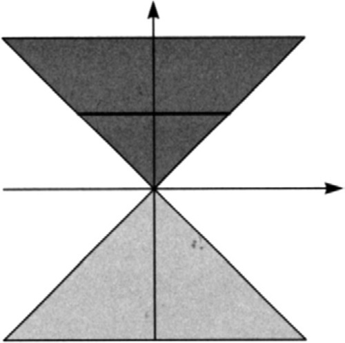
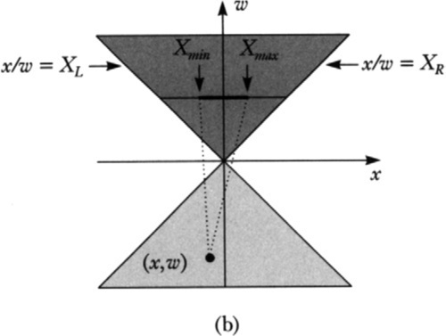
now let’s see how to calculate the screen extent of these hull points. (Actually, we are going to get the clip space extent; a simple scale and offset can turn this into pixel space.) For reference, let’s look at Figure 6.1 to see what’s happening in homogeneous space. For a more intuitive feel, you could also interpret this diagram as representing the situation before the perspective transformation by thinking of the w axis as the z axis (a perspective transformation sets w to the preperspective z value).

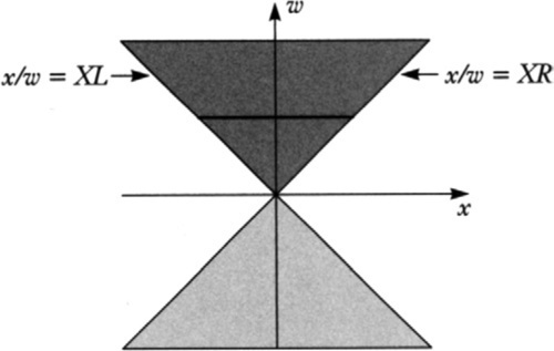
The darker gray region represents those points in front of the eye that project to the visible screen region (the dark line); this is where sLR==0. The lighter gray region represents the points that are behind the eye but would project into the screen region if we simply did the x/w divide. These points are, however, not visible.

We’ll calculate the screen extent by maintaining a running coverage range, Xmin and Xmax, and looping through the hull points, extending this range as necessary.

If sLR==0 for the next hull point, the situation is trivial; just update the range if the new point extends outside it.

if((x/w)<Xmin) Xmin=x/w;

if((x/w)>Xmax) Xmax=x/w;

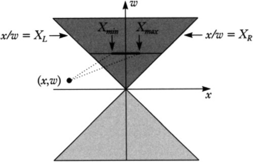
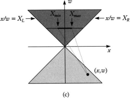
If sLR==Lout, the new point is in the left quadrant of the x, w plane (see Figure 6.2). All possible polygons connecting this new point with the current span will hit the left edge of the screen, so any points in this region should trigger an update of Xmin to push it out to the minimum value of XL. As an aside, note that if the point is in the negative w region of (sLR==Lout), then its projection will map to the right of the screen. This is an illusion of homogeneous perspective. All edges connecting it to the current range will only hit the left edge of the screen, and the update of Xmin=XL is still the correct thing to do.

The situation where sLR==Rout is symmetrical with sLR==Lout. Update Xmax to XR.

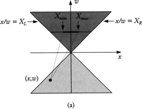
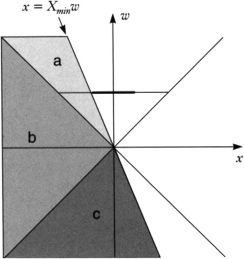
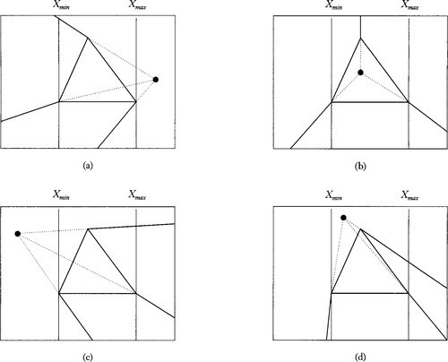
Now for the interesting situation: points in the light gray sLR==(Lout+Rout) region. There are three possible cases, depending on exactly where the new point is in the region.

In the first case, shown in Figure 6.3(a), the new hull point projects to a visible screen coordinate to the right of Xmax, but this is an illusion. In fact, all the visible points on the lines connecting the new point to the existing span will project to points to the left of Xmin. In this case, the appropriate action would be to extend Xmin to the left edge of the clip region, XL.

In the second case, Figure 6.3(b), all visible points connecting the new point to the existing span will project to points covering the whole screen. In this situation, the viewer is (potentially) inside the object. The appropriate action to take is to set Xmin to XL and to set Xmax to XR.

In the third case, Figure 6.3(c), all visible points connecting the new point to the existing span will project to points to the right of Xmax. So here we should set Xmax to XR.

The boundaries between cases 1 and 2 are where the rightmost dotted line passes through the origin, that is, where x/w=Xmax. The boundaries between cases 2 and 3 are where the leftmost dotted line passes through the origin, that is, where x/w=Xmin. Transliterating this into C++, we get

if (Xmax<x/w) Xmin=XL; //case 1

else if (Xmin<x/w<Xmax){Xmin=XL; Xmax=XR;} // case 2

else if (x/w<Xmin) Xmax=XR; // case 3

With a little fiddling, we can collapse this to actual legal C++.

if(Xmin<x/w) Xmin=XL; // case 1 and 2

if(x/w<Xmax) Xmax=XR; // case 2 and 3

Putting It Together

Combining all four cases, we get a first cut at the algorithm. Note that for the sLR==0 case, one or the other of the subsidiary if statements might be true, but not both. For the sLR== (Lout+Rout) case, at least one of the subsidiary if statements will be true and both might be.

if(sLR==0){

 if((x/w)<Xmin) Xmin=x/w;

 if((x/w)>Xmax) Xmax=x/w;}

if(sLR==Lout) Xmin=XL;

if(sLR==Rout) Xmax=XR;

if(sLR==Lout+Rout){

 if((x/w)=Xmin)  Xmin=XL;

 if((x/w)<Xmax)  Xmax=XR;}

Now we can make the following observation: whenever sLR==0, the value of w must be positive, so we can calculate ((x/w)<Xmin) as (x<Xmin*w). But what’s really interesting is that when sLR==Lout+Rout, the value of w must be negative, so we can also calculate ((x/w)>Xmin) as (x<Xmin*w). This gives us our next iteration.

if(SLR== 0){

 if(x<Xmin*w) Xmin=x/w;

 if(x>Xmax*w) Xmax=x/w;}

if(sLR==Lout)

 Xmin=XL;

if(sLR==Rout)

 Xmax=XR;

if(sLR==Lout+Rout){

 if(x<Xmin*w) Xmin=XL;

 if(x>Xmax*w) Xmax=XR;}

Finally, we can boil this down even further by first looking at Xmin and Xmax separately. For Xmin, the calculation is

if(SLR==0)

 if(x<Xmin*w) Xmin=x/w; // case a

if(sLR==Lout) Xmin=XL; // case b

if(sLR==Lout+Rout)

 if(x<Xmin*w) Xmin=XL; // case c

Figure 6.4 shows the three cases where Xmin changes. Notice that this only happens when x<Xmin*w and that in both cases b and c Xmin gets the same value, XL. This means that we can reduce the complexity of the code by reversing the order of the tests:

if(x<Xmin*w){

 if(sLR&Lout==0) Xmin=x/w; // case a

 else Xmin=XL;} // cases b and c

A similar analysis for the Xmax case gives

if(x>Xmax*w){

 if(sLR&Rout==0) Xmax=x/w;

 else Xmax=XR;}

Caveat

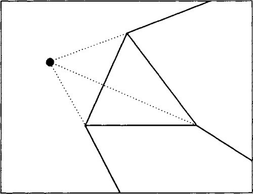
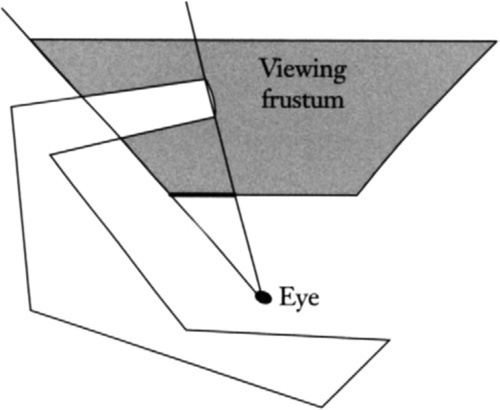
While this algorithm generates a rectangle that encloses the entire screen projection of the object, it sometimes generates a more conservative region than necessary. We must look at both x and y to see why. Suppose we have a tetrahedron whose base is in front of us but whose apex is behind us, say, to the right and downward. We can construct the screen region covered by the whole tetrahedron by projecting the apex through the eye onto the screen (now it’s to the left and upward), and drawing edges away from that point off to infinity, as shown in Figure 6.5.

Now let’s see what happens when we start with the Xmin and Xmax values from the visible base triangle and merge the apex point into the span. The three cases mentioned above are shown in Figures 6.6(a) through 6.6(c). In Figure 6.6(a) we have x/w>Xmin so Xmin is set to XL. This is fine. In Figure 6.6(b) we have x/w>Xmin so Xmin gets XL, and x/w<Xmax so Xmax gets XR. We are inside the tetrahedron. This is also fine. The situation in Figure 6.6(c) is basically symmetrical to that in 6.6(a): x/Xmax so Xmax gets XR. Also OK. The problem case is shown in Figure 6.6(d).

In Figure 6.6(d), since x/w is between Xmin and Xmax, both extents are extended to XL and XR. And, in fact, the polygon does stretch to infinity in the x direction. It is, however, clipped in y before it gets there. So, the region that is generated by the algorithm is more conservative than it needs to be. I’m not sure if this is a common situation though. And even if it is, things might not be so bad. Suppose that a hull point generates an overly conservative estimate using the current algorithm, but that we had a more complicated algorithm that considered the above situation and makes a better estimate. A later point in the hull array could quite possibly come along and expand the Xmin value back out to XL anyway.

Another Caveat

As another example of overconservativeness of the algorithm, recall that it finds the region covering the convex hull of the set of vertices. It is possible that concavities in the actual object might make for a situation where the covering rectangle is again too large. See Figure 6.7, which shows physical x and y in nonperspective space viewing a C-shaped structure. The algorithm would return the entire screen in this situation since the eye is inside the convex hull.

Summary

The algorithm developed here always returns a screen rectangle that is guaranteed to completely enclose the image of the 3D object. Sometimes, however, the rectangle is larger than absolutely necessary. I believe these situations are rare, but I am still doing some experimentation with real objects and viewing positions to really see if this happens often enough to worry about.