Search in book...
Toggle Font Controls
Create new playlist

Name your new playlist

Playlist description (optional)
Sign In

Email address

Password

Forgot Password?

or

Continue with Facebook

Continue with Google
Sign Up

Full Name

Email address

Confirm Email Address

Password

or

Continue with Facebook

Continue with Google

Chapter Fourteen

How Many Different Rational Parametric Cubic Curves Are There? Part I, Inflection Points

July–August 1999

In my never-ending quest to build intuition about the relationship between algebra and geometry, I have recently turned my attention once again to cubic curves. The basic question is this: what sorts of shapes can a given symbolic expression generate? In Chapter 4, “How Many Different Cubic Curves Are There?” and Chapter 6, “Cubic Curve Update,” of Jim Blinn's Corner: Dirty Pixels I asked this question about algebraic cubic curves of the form

$\begin{matrix} A x^{3} + 3 B x^{2} y + 3 C x y^{2} + D y^{3} \\ + 3 E x^{2} w + 6 F x y w + 3 G y^{2} w \\ ? + 3 H x w^{2} + 3 f y w^{2} \\ + K w^{3} = 0 \end{matrix}$

si1_e

I am now going to ask the same question about parametric cubic curves of the form

$[x ? (T) y ? (T) w ? (T)] = [T^{3} T^{2} T 1] ? [\begin{matrix} x_{3} & y_{3} & w_{3} \\ x_{2} & y_{2} & w_{2} \\ x_{1} & y_{1} & w_{1} \\ x_{0} & y_{0} & w_{0} \end{matrix}]$

si2_e

As an auxiliary question, I want to see which curve shapes can be generated both parametrically and algebraically. Many people have played around with this problem¹^,², what follows is my own personal take on the subject. I found out a lot of things that surprised me at first, but when I thought about them, they became pretty obvious. I hope I can make them obvious to you, too.

The parametric formula includes cubic Bezier curves, cubic B-spline curves, and so on, but those curves usually only consider a segment of the curve between the parameter values 0 and 1. In this chapter, I want to think about the whole curve as generated by all possible values of T from minus infinity to plus infinity. This holistic approach is guaranteed to generate points at infinity for some value of T or other. Therefore, in order to really understand what's going on with cubic curves, we must be fluent with infinity, both geometric and parametric. This means that we will generalize concepts that use Euclidean coordinates [X Y] into those that use projective homogeneous coordinates [x y w], and we will generalize the parameter T to the homogeneous parameter [t s].

Our ultimate goal will be to transform an arbitrary parametric cubic curve both geometrically and parametrically to match one of a set of canonical simple algebraic forms. How many such forms are possible? It turns out that there are exactly three. In order to see this, we will need some basic tools. The most important of these is the ability to find and catalog the inflection points of a curve. That will be the primary focus of this chapter.

Inflection Points

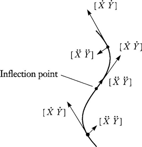
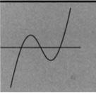
The main thing that a cubic curve can do, that lower-order curves cannot do, is have inflection points. What is an inflection point? Suppose you were driving a car along on the curve. An inflection point would be the place where you switch between “turning right” and “turning left.” Circles do not have inflection points. Sine curves have lots of them. We care about inflection points because they're preserved under perspective transformations. So two curves that differ only by a perspective transformation should have the same number of inflection points.

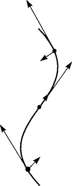
Algebraically, an inflection point occurs when the second derivative of the curve (the acceleration) is not, at time T, changing the direction of the first derivative (the tangent). See Figure 14.1. This occurs when the second derivative temporarily points in the same direction as the first derivative. A nonhomogeneous expression of this fact is

$[\dot{X} \dot{Y}] = α ? [\ddot{X} \ddot{Y}]$

si3_e

We don't really care what alpha is, so it's better to express our test as

$\frac{\dot{X}}{\ddot{X}} = \frac{\dot{Y}}{\ddot{Y}}$

$\dot{X} \ddot{Y} - \ddot{X} \dot{Y} = \det ? [\begin{matrix} \dot{X} & \dot{Y} \\ \ddot{X} & \ddot{Y} \end{matrix}] = 0$

si5_e

This determinant could also be zero, of course, if either the first or second derivative was itself zero. These locations aren't actually inflection points, but they will be useful special points to find, too.

f14-01-9781558608603 — Figure 14.1 Relation between inflection point and derivatives

We want to be able to deal fluidly with all possible points, both finite and infinite, so let's recast this in terms of homogeneous coordinates. For the X coordinate, our old friend the chain rule gives us

$\begin{matrix} X = \frac{x}{w} \\ \dot{X} = \frac{\dot{x} w - x \dot{w}}{w^{2}} \\ \ddot{X} = \frac{(\ddot{x} w - x \ddot{w}) ? w^{2} - (\dot{x} w - x \dot{w}) ? 2 w \dot{w}}{w^{4}} \end{matrix}$

si6_e

with similar expressions for Y. We can now write the 2×2 matrix in terms of homogeneous coordinates. Factoring out a few w's, we get

$\frac{1}{w^{2}} [\begin{matrix} \dot{x} w - x \dot{w} & \dot{y} w - y \dot{w} \\ (\ddot{x} w - x \ddot{w}) - 2 ? (\dot{x} w - x \dot{w}) \frac{\dot{w}}{w} & (\ddot{y} w - y \ddot{w}) - 2 ? (\dot{y} w - y \dot{w}) \frac{\dot{w}}{w} \end{matrix}]$

si7_e

Look at the mess on the second row and imagine what will happen to it as you take the determinant. You can see that the −2 (stuff) terms will cancel out. This leaves us with the much prettier

$\det ? [\begin{matrix} \dot{X} & \dot{Y} \\ \ddot{X} & \ddot{Y} \end{matrix}] = \frac{1}{w^{2}} \det ? [\begin{matrix} \dot{x} w - x \dot{w} & \dot{y} w - y \dot{w} \\ \ddot{x} w - x \ddot{w} & \ddot{y} w - y \ddot{w} \end{matrix}]$

si8_e

If you multiply out all the terms in this determinant and look at the result, you'll see a pattern. Several terms will cancel out and you will be left with six terms. A little thought and imagination, which I'll leave in your capable hands, will show that the inflection point-sensing determinant is equivalent to

$\det ? [\begin{matrix} \dot{x} w - x \dot{w} & \dot{y} w - y \dot{w} \\ \ddot{x} w - x \ddot{w} & \ddot{y} w - y \ddot{w} \end{matrix}] = w ? \det ? [\begin{matrix} x & y & w \\ \dot{x} & \dot{y} & \dot{w} \\ \ddot{x} & \ddot{y} & \ddot{w} \end{matrix}] = 0$

si9_e (14.1)

Second-Order Curves Can't Inflect

I claimed that a circle has no inflection points. More generally, no conic sections have inflection points. Let's see why by applying Equation (14.1) to a canonical second-order curve whose matrix representation looks like

$[x y w] = [T^{2} T 1] ? [\begin{matrix} x_{2} & y_{2} & w_{2} \\ x_{1} & y_{1} & w_{1} \\ x_{0} & y_{0} & w_{0} \end{matrix}]$

si10_e

To get the first and second derivatives of x, y, and w, you only need to differentiate the T row vector and conclude that

$[\begin{matrix} x & y & w \\ \dot{x} & \dot{y} & \dot{w} \\ \ddot{x} & \ddot{y} & \ddot{w} \end{matrix}] = [\begin{matrix} T^{2} & T & 1 \\ 2 T & 1 & 0 \\ 2 & 0 & 0 \end{matrix}] ? [\begin{matrix} x_{2} & y_{2} & w_{2} \\ x_{1} & y_{1} & w_{1} \\ x_{0} & y_{0} & w_{0} \end{matrix}]$

si11_e

Since the determinant of a product equals the product of the determinants, we have

$\begin{matrix} \det ? [\begin{matrix} x & y & w \\ \dot{x} & \dot{y} & \dot{w} \\ \ddot{x} & \ddot{y} & \ddot{w} \end{matrix}] = \det ? [\begin{matrix} T^{2} & T & 1 \\ 2 T & 1 & 0 \\ 2 & 0 & 0 \end{matrix}] \cdot \det ? [\begin{matrix} x_{2} & y_{2} & w_{2} \\ x_{1} & y_{1} & w_{1} \\ x_{0} & y_{0} & w_{0} \end{matrix}] \\ = - 2 \det ? [\begin{matrix} x_{2} & y_{2} & w_{2} \\ x_{1} & y_{1} & w_{1} \\ x_{0} & y_{0} & w_{0} \end{matrix}] \end{matrix}$

si12_e

All the T's canceled out. What does this mean? It means that the magic determinant is zero only if the coefficient matrix is singular, independent of T. A singular coefficient matrix means that the curve is degenerate; it's something like a circle squashed flat into a line segment. In this case, the tangent and second derivative point in the same direction along the whole curve. A nonsingular matrix, on the other hand, generates a full-fledged conic section. The magic determinant is never zero and therefore conic sections do not have inflection points.

Third-Order Curves Can

Now let's bump up to third-order curves and see what we can find out. Here we have

$[\begin{matrix} x & y & w \\ \dot{x} & \dot{y} & \dot{w} \\ \ddot{x} & \ddot{y} & \ddot{w} \end{matrix}] = [\begin{matrix} T^{3} & T^{2} & T & 1 \\ 3 T^{2} & 2 T & 1 & 0 \\ 6 T & 2 & 0 & 0 \end{matrix}] ? [\begin{matrix} x_{3} & y_{3} & w_{3} \\ x_{2} & y_{2} & w_{2} \\ x_{1} & y_{1} & w_{1} \\ x_{0} & y_{0} & w_{0} \end{matrix}]$

si13_e

What can we say about the determinant of this quantity? At first, it looks pretty scary. The final 3×3 matrix will have T-cubed terms on the top row, T-squared terms on the second row, and T terms on the bottom row. The determinant of this mess might potentially be sixth order in T. Eeeuw.

What was nice in the second-order discussion was that we could separately evaluate the part containing T and the part containing the polynomial coefficients because the determinant of the product of two matrices equals the product of their determinants. We can't take the determinants of the two matrices here since they aren't square. But we can do something similar. To introduce it, I'll start by dropping down a dimension and examine the product of a 2×3 matrix and a 3×2 matrix.

A Useful Identity

Let's look at the determinant of the simpler quantity

$\det ? ([\begin{matrix} P_{1} & P_{2} & P_{3} \\ Q_{1} & Q_{2} & Q_{3} \end{matrix}] ? ? [\begin{matrix} R_{1} & S_{1} \\ R_{2} & S_{2} \\ R_{3} & S_{3} \end{matrix}])$

si14_e

This notation makes it easy to think of the rows of the first matrix as two 3-vectors, P and Q, and think of the columns of the second matrix as two 3-vectors, R and S. The matrix product is then

$[\begin{matrix} P ? \cdot ? R & P ? \cdot ? S \\ Q ? \cdot ? R & Q ? \cdot ? S \end{matrix}]$

si15_e

and the determinant in question is

$\det ? ? [\begin{matrix} P ? \cdot ? R & P ? \cdot ? S \\ Q ? \cdot ? R & Q ? \cdot ? S \end{matrix}] ? ? = ? ? (P ? \cdot ? R) ? (? Q ? \cdot ? S ?) ? - ? (P ? \cdot ? S) ? (Q ? \cdot ? R)$

si16_e

When I first started playing with this, I multiplied everything out, took the determinant, and stared at the result for a while. A pattern began to emerge. The pattern I saw can be neatly summed up in the vector algebraic identity:

$? (P ? \cdot ? R) ? (? Q ? \cdot ? S ?) ? - ? (P ? \cdot ? S) ? (Q ? \cdot ? R ?) ? = ? (R \times S) ? \cdot ? (P \times Q)$

Upon further thought, I realized that this is just an expression of what is called the epsilon-delta rule. I expounded on this at length in Chapters 9 and 10, “Uppers and Downers” (Parts I and II) of Jim Blinn's Corner: Dirty Pixels. As desired, it allows us to turn the determinant of a matrix product into the product of two (almost) determinants (if you think of a cross product as a close relative of a determinant).

Up a Dimension

Now let's step up to the more heady world of 3×4 and 4×3 matrices. There is a 4D version of the epsilon-delta rule that uses a 4D analog to the cross product. The 4D cross product (which I'll call “crs₄”) takes three 4-vectors and generates a 4-vector that is perpendicular to each of them. You calculate the elements of this result by taking four determinants of three 3×3 matrices as follows:

$c r s_{4} ? ([\begin{matrix} x_{3} \\ x_{2} \\ x_{1} \\ x_{0} \end{matrix}]) ?, ? [\begin{matrix} y_{3} \\ y_{2} \\ y_{1} \\ y_{0} \end{matrix}] ?, ? [\begin{matrix} w_{3} \\ w_{2} \\ w_{1} \\ w_{0} \end{matrix}] ? = ? [\begin{matrix} D_{3} & D_{2} & D_{1} & D_{0} \end{matrix}]$

si18_e (14.2)

where

$\begin{array}{l} D_{3} ? = ? \det ? [\begin{matrix} x_{2} & y_{2} & w_{2} \\ x_{1} & y_{1} & w_{1} \\ x_{0} & y_{0} & w_{0} \end{matrix}] ?, ? D_{2} ? = ? - ? \det ? [\begin{matrix} x_{3} & y_{3} & w_{3} \\ x_{1} & y_{1} & w_{1} \\ x_{0} & y_{0} & w_{0} \end{matrix}] ?, \\ D_{1} ? = ? \det ? [\begin{matrix} x_{3} & y_{3} & w_{3} \\ x_{2} & y_{2} & w_{2} \\ x_{0} & y_{0} & w_{0} \end{matrix}] ?, ? D_{0} ? = ? - ? \det ? [\begin{matrix} x_{3} & y_{3} & w_{3} \\ x_{2} & y_{2} & w_{2} \\ x_{1} & y_{1} & w_{1} \end{matrix}] ?, \end{array}$

si19_e

In 3D, the cross product is perpendicular (has zero dot product) with the two input vectors. Similarly, the 4D cross product satisfies

$[\begin{matrix} D_{3} & D_{2} & D_{1} & D_{0} \end{matrix}] ? ? [\begin{matrix} x_{3} & y_{3} & w_{3} \\ x_{2} & y_{2} & w_{2} \\ x_{1} & y_{1} & w_{1} \\ x_{0} & y_{0} & w_{0} \end{matrix}] ? = ? [\begin{matrix} 0 & 0 & 0 \end{matrix}]$

si20_e

Note that the crs₄ of three column vectors is a row vector. Similarly, the crs₄ of three row vectors will be a column vector.

Let's give names to each row of the 3×4 matrix and to each column of the 4×3 matrix. The 4D epsilon-delta rule can be written in this form as

$\det ? ([\begin{matrix} \dots A \dots \\ \dots B \dots \\ \dots C \dots \end{matrix}] ? ? [\begin{matrix} ⋮ & ⋮ & ⋮ \\ X & Y & W \\ ⋮ & ⋮ & ⋮ \end{matrix}]) ? = ? {crs}_{4} ? ? (X, ? Y, ? W) ? \cdot ? {crs}_{4} ? ? (A, ? B, ? C)$

si21_e

In other words, the determinant of the matrix product is the dot product of the two 4D cross products. Again, I discussed this identity more fully in “Uppers and Downers.”

Application

Let's see what this tells us about the inflection points on the curve represented by the coefficient matrix. Our inflection point–finding determinant is

$\det ? [\begin{matrix} x & y & w \\ \dot{x} & \dot{y} & \dot{w} \\ \ddot{x} & \ddot{y} & \ddot{w} \end{matrix}] ? ? = ? ? \det ? ([\begin{matrix} T^{3} & T^{2} & T & 1 \\ 3 T^{2} & 2 T & 1 & 0 \\ 6 T & 2 & 0 & 0 \end{matrix}] ? ? [\begin{matrix} x_{3} & y_{3} & w_{3} \\ x_{2} & y_{2} & w_{2} \\ x_{1} & y_{1} & w_{1} \\ x_{0} & y_{0} & w_{0} \end{matrix}])$

si22_e

We can now separately evaluate the crs₄ of the T matrix to get

${crs}_{4} ? ? [\begin{matrix} T^{3} & T^{2} & T & 1 \\ 3 T^{2} & 2 T & 1 & 0 \\ 6 T & 2 & 0 & 0 \end{matrix}] ? ? = ? ? [\begin{matrix} - 2 \\ 6 T \\ - 6 T^{2} \\ 2 T^{3} \end{matrix}]$

si23_e

(I'll throw out the homogeneous factor of 2 from here on.) Next, the crs₄ of the coefficient matrix will be just the 4-element row of numbers $[\begin{matrix} D_{3} & D_{2} & D_{1} & D_{0} \end{matrix}]$ from Equation (14.2). We really can't say more about their values than that—they depend on what we were given for the coefficient matrix. The net result, then, is that an inflection point exists for each value of T that satisfies

$[\begin{matrix} D_{3} & D_{2} & D_{1} & D_{0} \end{matrix}] ? ? ? [\begin{matrix} - 1 \\ 3 T \\ - 3 T^{2} \\ T^{3} \end{matrix}] ? ? = ? ? D_{0} T^{3} - 3 D_{1} T^{2} + 3 D_{2} T - D_{3} = 0$

si25_e (14.3)

This is only third order in T rather than sixth order, as we originally feared. All the higher-order terms have conveniently canceled out.

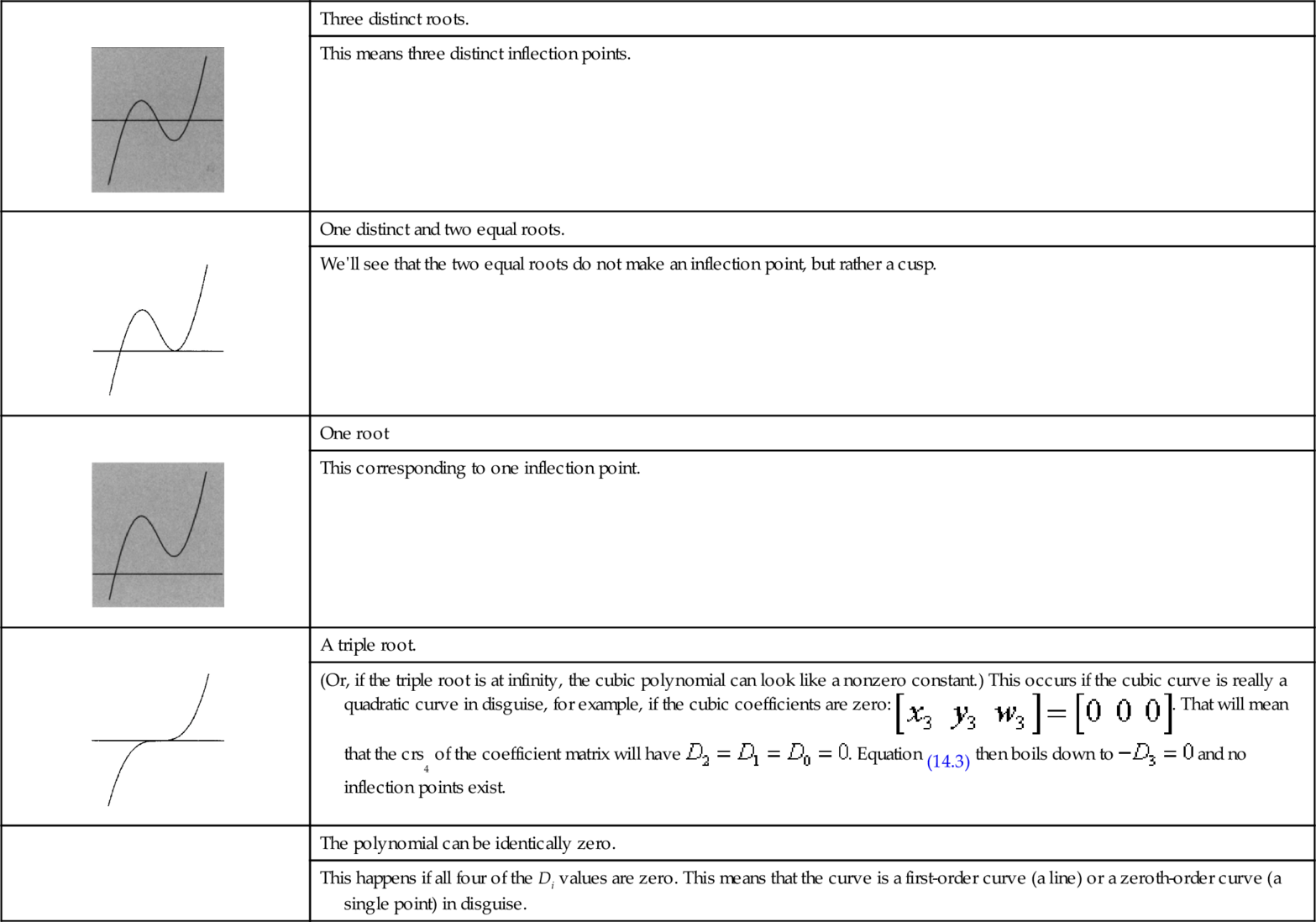
What does this mean? Since an inflection point lies at the solution of a cubic polynomial, the inflection point count does all the things that roots of cubic equations can do. The five possibilities appear in Table 14.1.

Table 14.1

Five different root structures of cubic equations

	Three distinct roots.
	This means three distinct inflection points.
	One distinct and two equal roots.
	We'll see that the two equal roots do not make an inflection point, but rather a cusp.
	One root
	This corresponding to one inflection point.
	A triple root.
	(Or, if the triple root is at infinity, the cubic polynomial can look like a nonzero constant.) This occurs if the cubic curve is really a quadratic curve in disguise, for example, if the cubic coefficients are zero: $[x_{3} y_{3} w_{3}] = [0 0 0]$ . That will mean that the crs₄ of the coefficient matrix will have $D_{2} = D_{1} = D_{0} = 0$ . Equation (14.3) then boils down to $- D_{3} = 0$ and no inflection points exist.
	The polynomial can be identically zero.
	This happens if all four of the D_i values are zero. This means that the curve is a first-order curve (a line) or a zeroth-order curve (a single point) in disguise.

t0010

Collinear Inflection Points

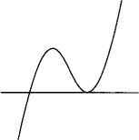
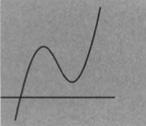
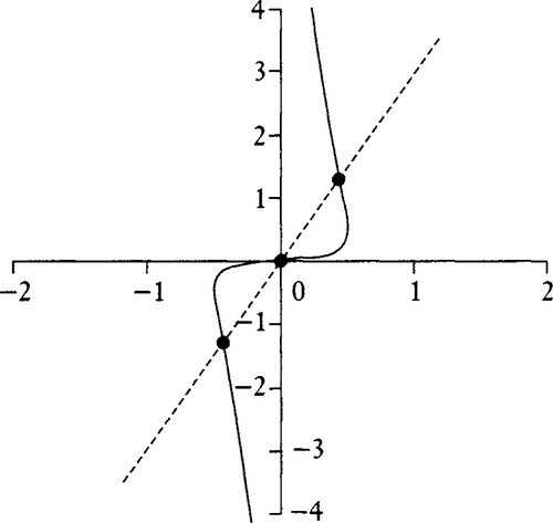
The epsilon-delta trick also gives us a quickie demonstration of the slightly surprising fact that, if three inflection points exist, then they must be collinear, as they are in Figure 14.2.

f14-02-9781558608603 — Figure 14.2 Cubic with three collinear inflection points

Suppose we have three solutions to the inflection point equation, T₀, T₁, T₂. Then the locations of the three inflection points I₀, I₁, I₂, stacked up into a matrix would be

$[\begin{matrix} T_{0}^{3} & T_{0}^{1} & T_{0} & 1 \\ T_{1}^{3} & T_{1}^{2} & T_{1} & 1 \\ T_{1}^{3} & T_{2}^{2} & T_{2} & 1 \end{matrix}] [\begin{matrix} x_{3} & y_{3} & w_{3} \\ x_{2} & y_{2} & w_{2} \\ x_{1} & y_{1} & w_{1} \\ x_{0} & y_{0} & w_{0} \end{matrix}] = [\begin{matrix} \dots I_{0} \dots \\ \dots I_{1} \dots \\ \dots I_{2} \dots \end{matrix}]$

si26_e

The condition that the three inflection points are collinear is that the determinant of the I matrix is zero. Look familiar? It's just the same situation as before. The determinant of the I matrix equals the dot product of the crs₄ of the other two. We already know the crs₄ of the coefficient matrix; it's $[\begin{matrix} D_{3} & D_{2} & D_{1} & D_{0} \end{matrix}]$ . What is the crs₄ of the matrix of T's? We could start taking 3×3 determinants and end up with a big mess of T₀'s, T₁'s, and T₂'s to various powers, but it turns out we already know the answer. The crs₄ is just a vector that is perpendicular to each row of the T matrix. Since the T_i's are solutions to Equation (14.3), we know that

$[\begin{matrix} T_{0}^{3} & T_{0}^{1} & T_{0} & 1 \\ T_{1}^{3} & T_{1}^{2} & T_{1} & 1 \\ T_{1}^{3} & T_{2}^{2} & T_{2} & 1 \end{matrix}] ? [\begin{matrix} D_{0} \\ - 3 D_{1} \\ 3 D_{2} \\ - D_{3} \end{matrix}] = [\begin{matrix} 0 \\ 0 \\ 0 \end{matrix}]$

si28_e

So we can evaluate the I determinant as a 4-vector dot product and find that it is identically zero:

$\det [\begin{matrix} \dots I_{0} \dots \\ \dots I_{1} \dots \\ \dots I_{2} \dots \end{matrix}] = [\begin{matrix} D_{3} & D_{2} & D_{1} & D_{0} \end{matrix}] ? [\begin{matrix} D_{0} \\ - 3 D_{1} \\ 3 D_{2} \\ - D_{3} \end{matrix}] = 0$

si29_e

So the three inflection points are indeed collinear.

The Case of the Missing Inflection Point

There is one more thing we need to do. Consider the following curve equation, which happens to be the one that generated Figure 14.2:

$[x y w] = [\begin{matrix} T^{3} & T^{2} & T & 1 \end{matrix}] ? [\begin{matrix} 0 & 0 & 1 \\ 1 & 0 & 0 \\ 0 & 0 & 1 \\ 0 & 1 & 0 \end{matrix}]$

si30_e

Now take the crs₄ of the coefficient matrix and plug it into Equation (14.3) and you get

$[1 0 - 1 0] ? [\begin{matrix} - 1 \\ 3 T \\ - 3 T^{2} \\ T^{3} \end{matrix}] = - 1 + 3 T^{2} = 0$

si31_e (14.4)

Fine. Two roots. What happened to the third inflection point? We can see three inflection points staring at us in Figure 14.2. Well … one of them is hidden at the parameter value T = ∞. This will happen for any curves that have D₀ = 0. How can we avoid missing such points? We handle infinite parameter values the same way we handle infinite geometric values, with homogeneous coordinates. Write the parameter T as a 1D homogeneous coordinate $t / s = T$ so that

$\begin{matrix} [\begin{matrix} T^{3} & T^{2} & T & 1 \end{matrix}] & = [\begin{matrix} \frac{t^{3}}{s^{3}} & \frac{t^{2}}{s^{2}} & \frac{t}{s} & 1 \end{matrix}] \\ = \frac{1}{s^{2}} ? [\begin{matrix} t^{3} & s t^{2} & s^{2} t & s^{3} \end{matrix}] \end{matrix}$

si33_e

Toss out the common homogeneous factor of ${1 / s}^{3}$ , and our homogeneous parametric curve definition is

$[x y w] = [t^{3} s t^{2} s^{2} t s^{3}] ? [\begin{matrix} x_{3} & y_{3} & w_{3} \\ x_{2} & y_{2} & w_{2} \\ x_{1} & y_{1} & w_{1} \\ x_{0} & y_{0} & w_{0} \end{matrix}]$

si35_e

How does this affect our location of inflection points? It just turns Equation (14.3) into

$[\begin{matrix} D_{3} & D_{2} & D_{1} & D_{0} \end{matrix}] ? [\begin{matrix} - s^{3} \\ 3 s^{2} t \\ - 3 s t^{2} \\ t^{3} \end{matrix}] = D_{0} t^{3} - 3 D_{1} s t^{2} + 3 D_{2} s^{2} t - D_{3} s^{3} = 0$

si36_e

In our problem case, Equation (14.4) becomes

$\begin{matrix} [1 0 - 1 0] ? [\begin{matrix} - s^{3} \\ 3 s^{2} t \\ - 3 s t^{2} \\ t^{3} \end{matrix}] & = - s^{3} + 3 s t^{2} \\ = s (\sqrt{3 t} + s) ? (\sqrt{3 t} - s) = 0 \end{matrix}$

si37_e

The three inflection points are, then, at the homogeneous parameters

$[t, ? s] = [1, 0], [1, - \sqrt{3}], [1, \sqrt{3}]$

The solution with s = 0 represents the inflection point at $T = t / s = \infty$ .

Next Time

The epsilon-delta rule lets us separate the algebra of the various derivatives of the parameters (which doesn't change from one curve to another) from the algebra on the polynomial coefficients (which does change). In the next chapter, armed with these tools, we'll tackle the problem of transforming an arbitrary parametric cubic to make its coefficient matrix have as many zeros as possible. We'll then look at how many patterns of nonzero elements remain and see what sorts of basic curve shapes are possible.

..................Content has been hidden....................

You can't read the all page of ebook, please click here login for view all page.

Table of Contents for Chapter Fourteen: How Many Different Rational Parametric Cubic Curves Are There? Part I, Inflection Points: July–August 1999

Create new playlist

Sign In

Sign Up