
Inferring Transforms
May-June 1999
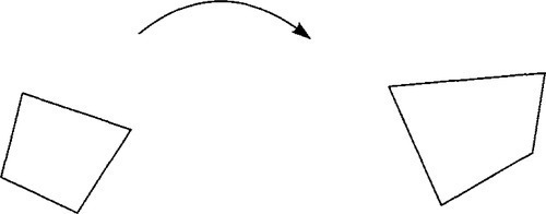
In simple 2D texture mapping, you take a 2D image and render it on the screen after some transformation or distortion. To accomplish this, you will need to take each [X, Y] location on the screen and calculate a [U, V] texture coordinate to place there. A particularly common transformation is
U=aX+bY+cgX+hY+j,V=dX+eY+fgX+hY+j
By picking the proper values for the coefficients a … j, we can fly the 2D texture around to an arbitrary position, orientation, and perspective projection on the screen. One can, in fact, generate the coefficients by a concatenation of 3D rotation, translation, scale, and perspective matrices, so we, of course, prefer the homogeneous matrix formulation of this transformation:
[XY1][adgbehcfj]=[uvw][UV]=[uwvw]
In this chapter, though, I'm going to talk about a more direct approach to finding a … j. It turns out that the 2D-to-2D mapping is completely specified if you give four arbitrary points in screen space and the four arbitrary points in texture space they must map to. The only restriction is that no three of the input or output points may be collinear. This method of transformation specification is useful, for example, in taking flat objects digitized in perspective and processing them into orthographic views.
Our Goal
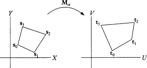
Let's make the problem explicit by giving names to some quantities. We are given four 2D screen coordinates si=[XiYi1]![]() and four 2D texture coordinates ti=[UiVi1]
and four 2D texture coordinates ti=[UiVi1]![]() , and we want to find the 3 × 3 homogeneous transformation Mst that maps one to the other so that
, and we want to find the 3 × 3 homogeneous transformation Mst that maps one to the other so that
siMst=witi
See Figure 13.1. Note that we are not given the wi values. Their participation in Equation (13.1) acknowledges the fact that even though the original input and output points are nonhomogeneous (their third component is 1), the output of the matrix multiplication will be homogeneous. We will have to solve for the w values as a side effect of solving for the elements of Mst.
The Conventional Solution
The conventional way to solve this goes as follows. First, using the names a … j for the elements of Mst, we can rewrite Equation (13.1) explicitly as
[XiYi1][adgbehcfj]=wi[UiVi1]
Multiplying out and equating each component gives us three equations:
aXi+bYi+c=wiUidXi+eYi+f=wiVigXi+hYi+j=wi
Plug the last equation for wi into the first two and move everything to the left of the equal sign:
aXi+bYi+c−gXiUi−hYiUi−jUi=0dXi+eYi+f−gXiVi−hYiVi−jVi=0
Write this as yet another matrix equation in terms of what we are solving for, a … j:
[XiYi1000−XiUi−YiUi−Ui000XiYi1−XiV−YiVi−Vi][abcdefghj]=[00]
Each input point gives us two more 9-element rows; four points gives us an 8 × 9 matrix. Since this is a homogeneous system, that's all we need to solve for the nine values a … j (with an arbitrary global scale factor). One way to calculate each of these nine values is to find the determinant of the 8 × 8 matrix formed by deleting the matching column of the 8 × 9 matrix, so … nine determinants of 8 × 8 matrices. This is doa ble but obnoxious. Looking at all those lovely zeros and ones on the left makes us suspect that there is a better way.
Heckbert's Improvement
In his 1989 master's thesis, Paul Heckbert1 made a great leap by splitting the transformation into two separate matrices. He first used one matrix to map the input points to a canonical unit square (with vertices [0, 0], [1, 0], [1, 1], [0, 1]) and then mapped that square into the output points with another matrix. See Figure 13.2.
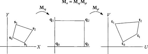
Each of these matrices will be individually easier to calculate than the complete transformation since the arithmetic is so much simpler. In fact, the arithmetic turns out to be simplest for the second of these transformations, so we will solve that one explicitly. Naming points in the unit-square space q, we want to find Mqt in the equation
qMqt=wtt
![]()
Let's explicitly write out all components for all four input/output (q/t) point pairs. I'll recycle the names a … j and w0 … w3 for use in this subcomputation, so be aware that their values are different from those I used in the “conventional” solution:
[001101111011][adgbehcfj]=[w0U0w0V0w0w1U1w1V1w1w2U2w2V2w2w3U3w3V3w3]
This generates 12 equations:
c=w0U0f=w0V0j=w0a+c=w1U1d+f=w1V1g+j=w1a+b+c=w2U2d+e+f=w2V2g+h+j=w2b+c=w3U3e+f=w3V3h+j=w3
Substituting the right column of equations into the left two columns gives us
c=jU0f=jV0a+c=(g+j)U1d+f=(g+j)V1a+b+c=(g+h+j)U2d+e+f=(g+h+j)V2b+c=(h+j)U3e+f=(h+j)V3
Then substituting the equations in rows 1, 2, and 4 into the third row gives the two equations
(g+j)U1+(h+j)U3−jU0=(g+h+j)U2(g+j)V1+(h+j)V3−jV0=(g+h+j)V2
We juggle this into
g(U1−U2)+h(U3−U2)=j(U0−U1+U2−U3)g(V1−V2)+h(V3−V2)=j(V0−V1+V2−V3)

Heckbert's original solution did the “without loss of generality” trick and assumed that j = 1. This works since we can only expect to solve for the matrix elements up to some global scalar multiple, and since j cannot be zero if point 0 is not at infinity. He then solved for g and h and got something that looked like
g=det[stuff0]det[stuff2]h=det[stuff1]det[stuff2]
I don't really like the j = 1 assumption though since it leads to these nasty divisions. And we really don't need it if we think homogeneously. We can instead write Equation (13.3) as
[ghj][U1−U2V1−V2U3−U2V3−V2−U0+U1−U2+U3−V0+V1−V2+V3]=[00]
And just say that the vector [g h j] is the cross product of the two columns of the above matrix. This gives us, after a little simplification
g=(U3−U2)(V1−V0)−(U1−U0)(V3−V2)h=(U3−U0)(V1−V2)−(U1−U2)(V3−V0)j=(U1−U2)(V3−V2)−(U3−U2)(V1−V2)

Once we have these, it's a simple matter to get a through f using Equation (13.2):
c=jU0f=jV0a=(g+j)U1−cd=(g+j)V1−fb=(h+j)U3−ce=(h+j)V3−f
Now that we have Mqt, the same simple arithmetic will give us the mapping from the canonical square to the input points. This will be the matrix that satisfies:
qMqs=wss
![]()
Invert that (or, better, take its adjoint) and multiply to get our desired net matrix:
Mst=[Mqs]∗Mqt
![]()
Olynyk's Improvement
An even better solution recently came from my colleague Kirk Olynyk here at Microsoft Research. His basic idea was to use barycentric coordinates, rather than a unit square, as the intermediate system. Barycentric coordinates represent an arbitrary point in the plane as the weighted sum of three basis points, for example, the first three of our output points. This would represent an arbitrary texture coordinate t as
τ0t0+τ1t1+τ2t2=t
![]()
with the constraint that the barycentric coordinates sum to one: τ0+τ1+τ2=1![]() . Similarly, we can represent an arbitrary input point in barycentric coordinates as
. Similarly, we can represent an arbitrary input point in barycentric coordinates as
σ0s0+σ1s1+σ2s2=s
![]()
Kirk then related the two barycentric coordinate systems by coming up with a mapping from [σ0σ1σ2]![]() to [τ0τ1τ2]
to [τ0τ1τ2]![]() that has the property that the barycentric coordinates of all four input points map to the barycentric coordinates of their respective output points. That is,
that has the property that the barycentric coordinates of all four input points map to the barycentric coordinates of their respective output points. That is,
[100]↦[100][010]↦[010][001]↦[001][˜σ0˜σ1˜σ2]↦[˜τ0˜τ1˜τ2]
(The two points in the fourth mapping above are the barycentric coordinates of the fourth input/output point pair.) To get the desired mapping, simply multiply each σi, componemt of an arbitrary input point by ˜τi/˜σi![]() . Then renormalize to a valid barycentric coordinate by dividing by the sum of the components. You can see that this algorithm leaves the coordinates of the first three points intact while properly changing those of the fourth point.
. Then renormalize to a valid barycentric coordinate by dividing by the sum of the components. You can see that this algorithm leaves the coordinates of the first three points intact while properly changing those of the fourth point.
So how do we get the barycentric coordinates of the fourth input/output pair? Start with the matrix formulation of the barycentric coordinates of an arbitrary point. Here's the one for output points:
[τ0τ1τ2][U0V01U1V11U2V21]=t
Note that if τ0+τ1+τ2=1![]() , this guarantees that the w (homogeneous) component of t will be 1 also. Anyway, plugging in t = t3 and moving the matrix over the equal sign gives us
, this guarantees that the w (homogeneous) component of t will be 1 also. Anyway, plugging in t = t3 and moving the matrix over the equal sign gives us
[˜τ0˜τ1˜τ2]=[U3V31][U0V01U1V11U2V21]−1
This is nice, but it's not ideal. A full-on matrix inversion requires division by the determinant of the matrix. Likewise, the normalization to unit-sum barycentric coordinates requires division by the sum of the coordinates. Kirk dislikes divisions even more than I do, so in his implementation he removed them by homogeneously scaling them out symbolically after the fact. In thinking about this solution, though, I realized that there is a different way of deriving it that better shows its relation to the Heckbert solution.
Another Interpretation
Heckbert used a unit square as an intermediate coordinate system, and Olynyk used barycentric coordinates. Let's look at this problem anew and try to pick an intermediate coordinate system (call it b) that will minimize our arithmetic as much as possible when we solve for Mbt in the equation
bMbt=wt
![]()
We want four points bi in our new coordinate system that have as many zeros as possible as components. The four simplest (homogeneous) points I can imagine are [1 0 0], [0 1 0], [0 0 1], and [1 1 1]. It doesn't matter that two of these are points at infinity. All that matters is that no three of these points are collinear. I show this new two-stage transformation in Figure 13.3, although it might be a bit confusing (and unnecessary) to try to make a closed quadrilateral out of the four b points.
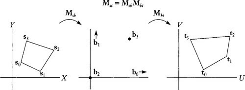
The b coordinate system is like “homogeneous barycentric coordinates” (with the restriction relaxed that the sum of the components equals one) but is further scaled so that the components of the fourth point are equal.
So let's solve for Mbt Being extremely ecological, I will again recycle the names a … j for the matrix elements and w0 … w3 for the (as yet) unknown homogeneous factors. Our four points generate
[100010001111][adgbehcfj]=[w0U0w0V0w0w1U1w1V1w1w2U2w2V2w2w3U3w3V3w3]
We could solve this by doing the same sort of substitutions that we did in the Heckbert solution, but there's an easier way. Looking at the top three rows on each side, we immediately realize that we have Mbt already staring us in the face; it's just the first three rows of Equation (13.5). Let's write it in factored form:
Mbt=[adgbehcfj]=[w0000w1000w2][U0V01U1V11U2V21]
We only need to find w0, w1, and w2, and we are home free. To get these, we take the bottom row of Equation (13.5):
[111]Mbt=[w3U3w3V3w3]
![]()
and combine it with Equation (13.6) and write
[111][w0000w1000w2][U0V01U1V11U2V21]=w3[U3V31]
We can hop the UV matrix over the equal sign by inverting it to get
[w0w1w2]=w3[U3V31][U0V01U1V11U2V21]−1
Comparing Equation (13.7) with Equation (13.4), we can see the relationship
[w0w1w2]=w3[˜τ0˜τ1˜τ2]
In other words, our w0 … w2 values are just a homogeneous scaling of the pure barycentric coordinates of the fourth point. Note also that the right-hand column of Equation (13.5) tells us that
w0+w1+w2=w3
Remember that we can determine the w's only up to a homogeneous scale factor, so let's pick something nice for, say, w3. How about using the determinant of the matrix we are inverting? This can never be zero if the three points t0, t1, and t2 aren't collinear. Letting w3 equal this matrix determinant would pleasantly turn the matrix inverse into a matrix adjoint and we have
[w0w1w2]=[U3V31][U0V01U1V11U2V21]∗
So … that's half of our final answer. Now for the other half, the matrix Msb. We get the inverse of Msb by doing the same calculation using the four input coordinate points. First calculate the three homogeneous scale factors, which I'll call z, by analogy with Equation (13.9):
[z0z1z2]=[X3Y31][X0Y01X1Y11X2Y21]∗
And then, by analogy with Equation (13.6):
Mbs=[z0000z1000z2][X0Y01X1Y11X2Y21]∗
To arrive at our ultimate goal of Mst, we need the adjoint of Mbs. One very nice feature of the factored form of the matrix that I've written here is that it's arithmetically simpler to adjointify than a general matrix. I'll write it out explicitly:
[Mbs]∗=[Y1−Y2Y2−Y0Y0−Y1X2−X1X0−X2X1−X0X1Y2−X2Y1X2Y0−X0Y2X0Y1−X1Y0][z1z2000z0z2000z0z1]
Put 'em all together and we get our gigantic punch line:
Mst=[Mbs]∗Mbt
![]()
Now it's time to name some of the matrices I've been laboriously writing out for so long (actually, I've been cutting and pasting). Up to this point, I've felt that explicitly writing them out has been more informative since it allows comparisons with other parts of the equation. I will name the following matrices:
T≡[U0V01U1V11U2V21]S≡[X0Y01X1Y11X2Y21]
Finally, let's rewrite our final answer slightly to give a nice comparison of this technique with (a homogenized version of) Kirk's original solution:
Mst=S∗[w0z1z2000z0w1z2000z0z1w2]T
The matrix S* takes us from screen space to (homogeneous) barycentric coordinates. The w and z diagonal matrices combine to give one diagonal matrix whose elements are just homogeneous scalings of the ˜τi/˜σi![]() quantities that Kirk used to go from the screen barycentric system to the texture barycentric system. Matrix T then takes us to texture coordinates. This form is almost the simplest we can do arithmetically. But let's not give up yet.
quantities that Kirk used to go from the screen barycentric system to the texture barycentric system. Matrix T then takes us to texture coordinates. This form is almost the simplest we can do arithmetically. But let's not give up yet.
Geometric Interpretations
As Equations (13.9) and (13.10) indicate, we need the adjoints of matrices T and S to calculate the w and z values to plug into Equation (13.12). The adjoint S* also shows up in Equation (13.12), but we only use T* to calculate the w's. Let's look at this w calculation, then, to see if there's some way we can save ourselves some work. While this investigation is initially motivated by performance avarice, it will actually point out some geometric relationships that I think are the most interesting results of this whole problem. In other words, greed is good.
First, let's use the definition in Equation (13.9) to explicitly write out the calculation of w0:
w0=U3(V1−V2)+V3(U2−U1)+(U1V2−U2V1)
What does this mean? Well, each row of matrix T is a point, one of t0, t1 or t2. According to the definition of the adjoint, each column of T* is the cross product of two rows (points) of T. This means that each column of T* is a homogeneous line. For example, column 0 of T*represents the line connecting points t1 and t2. The process of multiplying an arbitrary point t by the matrix T* just takes its dot product with the three lines t1t2, t2t0, and t0t1. In other words, it measures the distance from the point to the three lines. That's the essential meaning of barycentric coordinates. In any event, we can now rewrite Equation (13.13) as
w0=t3⋅t1×t2
![]()
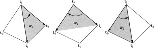
This common algebraic expression has a standard geometric interpretation. Thinking of t1, t2, and t3 as 3D vectors, it's the volume of the parallelepiped they define. Thinking, however, of the three points as homogeneous 2D vectors, there's another interpretation: w0 equals twice the area of the triangle t3t2t1. We can verify this algebraically by comparing the definition of w0 from Equation (13.13) with twice the integral under the three triangle edges:
w0=(U1−U2)(V1+V2)+(U2−U3)(V2+V3)+(U3−U1)(V3+V1)
But there's another way to calculate triangle areas: as (half) the length of a cross product. We can rewrite our expression for w0 so that it looks like a cross product of two vectors along the edges of the triangle. For example, taking the third component of the cross product of the vectors (t1 − t3) and (t1 − t2) gives us
w0=(U1−U3)(V2−V3)−(U2−U3)(V1−V3)
![]()
Now let's calculate w1 (which is half the area of triangle t3t0t2) and w2 (half the area of triangle t3t1t0). We only need one more vector difference: (t0 − t3). This gives the simplest way I've found to calculate all the W's:
w0=(U1−U3)(V2−V3)−(U2−U3)(V1−V3)w1=(U2−U3)(V0−V3)−(U0−U3)(V2−V3)w2=(U0−U3)(V1−V3)−(U1−U3)(V0−V3)
Again, you can verify algebraically that these expressions equal those from Equation (13.9), but the geometric arguments make it seem a bit less magical. Also, you can look at Figure 13.4 for some more geometric inspiration.
One more Thin Little mint
There's one last little bit of juice we can squeeze out of this. This, again, came from Kirk, but he found it purely algebraically. I'm going to motivate it by an even more interesting geometric observation. It turns out that there is a magical relationship between the zi values and the bottom row of S*. So we have to switch gears and start talking, not about U, V,w but about X,Y,z. I'll write the analog to Equation (13.14) and, for good measure, throw in a formula for z3, which is, by analogy with Equation (13.8), the sum of the first three:
z0=(X1−X3)(Y2−Y3)−(X2−X3)(Y1−Y3)z1=(X2−X3)(Y0−Y3)−(X0−X3)(Y2−Y3)z2=(X0−X3)(Y1−Y3)−(X1−X3)(Y0−Y3)z3=(X1−X0)(Y2−Y0)−(X2−X0)(Y1−Y0)
We can now see the missing link: the geometric interpretation of the value z3. It's the area of triangle s0s1s2. To see this, look at Figure 13.5 and note that z0 plus z2 equals the area of the whole quadrilateral. Now look at z1. Since its edge vectors sweep clockwise, that area is negative and subtracts from the quadrilateral to get triangle s0s1s2.
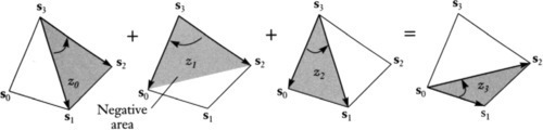
One side note: the area of the whole quadrilateral is
z0+z2=−z1+z3=(X1−X3)(Y2−Y0)−(X2−X0)(Y1−Y3)
![]()
This reminds us that the area of the quadrilateral is (twice) the cross product of its diagonals (with appropriate care in algebraic sign).
Now let's take a look at the bottom row of S* (inside Equation (13.11)). Again, these look like areas of some sort. In fact, they are the areas of the three triangles connecting the three edges of triangle t0t1t2 with the origin. (If this isn't immediately clear, try temporarily imagining point 3 at the origin.) The sum of these areas also equals z3, so we have the following identity, which you can also verify algebraically:
S*20+S*21+S*22=z3
![]()
This means that
S*20+S*21+S*22=z0+z1+z2
![]()
So we can calculate one of the z's in terms of the others. This can, for example, turn the calculation
z0=X3S*00+Y3S*10+S*20
![]()
into
z0=S*20+S*21+S*22−z1−z2
![]()
It turns two multiplications into two additions. This may, or may not, be a particularly big deal with current processors.
Code
// Calculate elements of matrix Mst
// From 4 coordinate pairs
// (Ui Vi), (Xi Yi)
U03 = U0-U3; V03 = V0-V3;
U13 = U1-U3; V13 = V1-V3;
U23 = U2-U3; V23 = V2-V3;
w0 = U13*V23 - U23*V13;
wl = U23*V03 - U03*V23;
w2 = U03*V13 - U13*V03;
Sa00 = Y1-Y2; Sa10 = X2-X1;
Sa01 = Y2-Y0; Sa02 = Y0-Y1;
Sa11 = X0-X2; Sa12 = X1-X0;
Sa20 = X1*Y2 - X2*Y1;
Sa21 = X2*Y0 - X0*Y2;
Sa22 = X0*Y1 - X1*Y0;
z1 = X3*Sa01 + Y3*Sa11 + Sa21;
z2 = X3*Sa02 + Y3*Sa12 + Sa22;
z0 = Sa20+Sa21+Sa22 - z1 - z2;
d0 = w0*zl*z2;
d1 = wl*z2*z0;
d2 = w2*z0*z1;
Sa00*=d0; Sa10*=d0; Sa20*=d0;
Sa01*=d1; Sa11*=d1; Sa21*=d1;
Sa02*=d2; Sa12*=d2; Sa22*=d2;
M00 = Sa00*U0 + Sa01*U1 + Sa02*U2;
M10 = Sa10*U0 + Sa11*U1 + Sa12*U2;
M20 = Sa20*U0 + Sa21*U1 + Sa22*U2;
M01 = Sa01*V0 + Sa01*Vl + Sa02*V2;
M11 = Sa11*V0 + Sa11*V1 + Sa12*V2;
M21 = Sa21*V0 + Sa21*V1 + Sa22*V2;
M02 = Sa00 + Sa01 + Sa02;
M12 = Sa10 + Sa11 + Sa12;
M22 = Sa20 + Sa21 + Sa22;
Down a Dimension
As a mental exercise, let's look at this problem in one dimension. Suppose we want to find a single function relating X and U of the form
U=aX+bcX+d
In matrix notation, this would be
[X1][acbd]=w[U1]
Here, each input/output pair (Xi and Ui) gives us one row in the expression
[Xi1−XiUi−Ui][abcd]=0
Three input/output pairs generate enough rows on the left to make this a fully determined system. Solving for a … d requires the determinants of four 3 × 3 matrices. But applying our 2D trick to the 1D problem, we can get the same result by the calculation
[w0w1]=[(U1−U2)(U2−U0)][z0z1]=[(X1−X2)(X2−X0)][acbd]=[1−1−X1X0][z1w000z0w1][U01U11]
Tediously multiplying this out gives the following:
a=U0X0(U2−U1)+X1U1(U0−U2)+X2U2(U1−U0)b=X0X1U2(U1−U0)+X1X2U0(U2−U1)+X2X0U1(U0−U2)c=X0(U2−U1)+X1(U0−U2)+X2(U1−U0)d=X0X1(U1−U0)+X1X2(U2−U1)+X2X0(U0−U2)
The patterns in these expressions explicitly show something that we expect and implicitly assumed: the transformation will come out the same if we permute the indices of the input/output point pairs.
We will use this 3-point to 3-point transformation to great effect in the next few chapters.
Up a Dimension
Now, close your eyes and stretch your mind in the other direction. Imagine input/output pairs in homogeneous 3D space. Each pair, connected by a 4 × 4-element matrix multiplication, gives four equations. The fourth equation gives an expression for wi Plug it into the other three and rearrange to get three equations that can be written as three rows of stuff times a 16-element column of matrix elements a … p. Since this has a zero on the right side, we need one less than 16 equations to solve the homogeneous system. Hmm, 16 minus 1 gives 15, and we get three per input/ output pair. That means that we can nail down a 3D homogeneous perspective transform with five input/output pairs. The conventional solution requires a truly excruciating 16 determinants of 15 × 15 matrices. Opening your eyes in shock, you discover that this exercise in imagination allowed me to get the idea across without making the typesetter hate me.
But now we know better how to solve this. The answer is a fairly straightforward generalization of Equations (13.6) and (13.9) into 4 × 4 matrices and 4-element vectors like so:
Mbt=[w00000w10000w20000w3][U0V0T01U1V1T11U2V2T21U3V3T31][w0w1w2w3]=[U4V4T41][U0V0T01U1V1T11U2V2T21U3V3T31]∗
The details and arithmetic optimization tricks are left as an exercise for you to do (meaning I haven't gotten around to doing it myself).