The Basic Objects

Since this chapter is mostly about C++, I will review just enough of the algebra to motivate the code. We are interested in algebraic curves defined by F(x, y, w) = 0. The simplest of these is a straight line, represented by the equation

$Ax+By+Cw=0$

A quadratic curve is represented by the equation

$\begin{array}{ccc}\hfill A{x}^2+2By+2Cxw& \hfill & \hfill \\ \hfill +D{y}^2+2Eyw& \hfill & \hfill \\ \hfill +F{w}^2& \hfill =& \hfill 0\end{array}$

A cubic curve is represented by the equation

$\begin{array}{ccc}\hfill A{x}^3+3B{x}^{2}y+3Cx{y}^2+D{y}^3& \hfill & \hfill \\ \hfill +3E{x}^{2}w+6Fxyw+3G{y}^{2}w& \hfill & \hfill \\ \hfill +3Hx{w}^2+3\mathcal{J}y{w}^2& \hfill & \hfill \\ \hfill +K{w}^3& \hfill =& \hfill 0\end{array}$

We want to relate various geometric properties of these curves with algebraic combinations of the coefficients A…K. The first step is to arrange the coefficients in arrays that, in mathematical lingo, are called tensors. For a line, we arrange the coefficients into a column vector:

$\text{L}=\left[\begin{array}{c}A\\ B\\ C\end{array}\right]$

For the quadratic, we define the symmetric matrix

$\text{Q}=\left[\begin{array}{ccc}A& B& C\\ B& D& E\\ C& E& F\end{array}\right]$

For the cubic curve equation, we arrange the coefficients into a 3 × 3 × 3 tensor that we can write (clumsily) as a vector of matrices:

$\text{C}=\left[\left[\begin{array}{ccc}A& B& E\\ B& C& F\\ E& F& H\end{array}\right]\left[\begin{array}{ccc}B& C& F\\ C& D& G\\ F& G& \mathcal{J}\end{array}\right]\left[\begin{array}{ccc}E& F& H\\ F& G& \mathcal{J}\\ H& J& K\end{array}\right]\right]$

When we write an element of one of these tensors, the convention is to label its location in the array with indices written as subscripts. These are called covariant indices and look like

$L_i,Q_{ij},C_{ijk}$

A point, on the other hand, is written as a row vector:

$P=[xyw]$

When we write an element of the point, we label it with an index written as a superscript. (This does not mean exponentiation. It's just a place to put the index.) These indices are called contravariant and look like

$P^i$

Finally, we will have use for a constant 3 × 3 × 3 contravariant tensor called epsilon whose elements are defined to be

$\begin{array}{ccc}\hfill {\epsilon }^{012}={\epsilon }^{120}={\epsilon }^{201}& \hfill =& +1\hfill \\ \hfill {\epsilon }^{210}={\epsilon }^{021}={\epsilon }^{102}& \hfill =& -1\hfill \\ \hfill {\epsilon }^{ijk}& \hfill =& 0\text{otherwise}\hfill \end{array}$

The Basic Operation

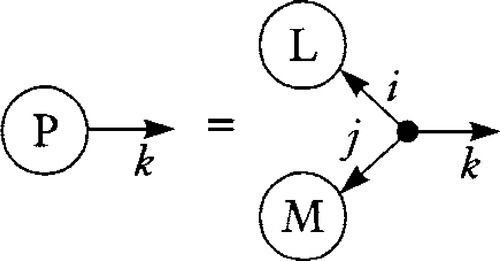
The basic quantity we want to calculate is a “contraction” of two or more tensors. Vector dot products and vector/matrix products are special cases of tensor contractions. More generally, we want to evaluate expressions such as

${\displaystyle \sum _{ijklmn}{\epsilon }^{ijk}{\epsilon }^{lmn}{\text{Q}}_{il}{\text{Q}}_{jm}{\text{Q}}_{kn}}$

And, being lazy, we will abbreviate expressions like Equation (21.1) by leaving out the summation sign. Any index that appears exactly twice in an expression, once as covariant and once as contravariant, will be assumed summed over.

So, I want to come up with a simple symbolic algebra manipulation program that is good at these sorts of expressions and doesn't really need to handle anything more general. We saw in Chapter 20 that Equation (21.1) should evaluate to six times the determinant of Q. So if we translate Equation (21.1) into C++ code, we want the program to print out something like this:

$6ADF+12BCE-6C^{2}D-6A{E}^2-6B^{2}F$

Incidentally, if this polynomial is zero, it tells us that the quadratic is really the product of two linear factors—that is, the equation stands for two straight lines.

The Epsilon Routine

The most obvious first step is to define a routine to calculate epsilon as follows:

int epsilon(int i, int j, int k)

{

 if(i==0 && j==1 && k==2) return 1;

 if(i==1 && j==2 && k==0) return 1;

 if(i==2 && j==0 && k==1) return 1;

 if(i==2 && j==1 && k==0) return −1;

 if(i==0 && j==2 && k==1) return −1;

 if(i==1 && j==0 && k==2) return −1;

 return 0;

}

We are ultimately going to define a class Polynomial to hold the final answer and a subroutine Q (i, j) that returns the symbolic value in element i, j. If we design these properly, we can write code to evaluate Equation (21.1) that simply loops through all values of i, j, k, l, m, n and adds up the terms, like so (note that I am using the STL-like convention for loop bounds).

#define forIndex(I) for(int I=0;I!=3;++I)

Polynomial E;

forIndex (i)

forIndex (j)

forIndex (k)

forIndex (l)

forIndex (m)

foIndex (n)

E += epsilon(i, j, k)*epsilon(l, m, n)*Q(i, l)*Q(j, m)*Q(k,n) ;

cout << E << endl;

This, however, gets out of hand pretty quickly. The epsilon tensor is mostly zeros; in fact, only 6 out of the 27 entries are nonzero (or $\raisebox{1ex}{$2$}\!\left/ \!\raisebox{-1ex}{$9$}\right.$ of them). If you have two epsilons in your expression, then only 6*6 out of the 27*27 possible combinations are nonzero (about 1 in 20). Some of the diagrams we will be ultimately interested in can have eight or more epsilons. This means that only 6⁸ out of the 27⁸ iterations (about 1 in 168,151) actually adds anything to E. And for each epsilon, you have three nested loops. There must be a better way.

There is. We'll turn the loops inside out. Instead of generating all combinations of indices, we will have each loop go through the six nonzero epsilon values and return to us their indices and signs. The new epsilon function looks like

int epsilon (int which, int* pI, int* pJ, int* pK)

{

static int Ix1[6] = {0,1,2,2,0,1};

static int Ix2[6] = {1,2,0,1,2,0};

static int Ix3[6] ={2,0,1,0,1,2};

static int Sgn[6] ={1,1,1,−1,−1,−1};

 *pI=Ix1[which];

 *pJ=Ix2[which];

 *pK=Ix3[which];

 return Sgn[which];

}

And the loop to evaluate Equation (21.1) will look like

#define forEpsilon(e) for (int e=0; e!=6; ++e)

Polynomial P;

forEpsilon(e1)

forEpsilon(e2)

{

 int i, j, k, l, m, n;

 int sign=epsilon(e1,&i,&j,&k)

 *epsilon(e2,&l,&m,&n);

 P += sign*Q(i,l)*Q(j,m)*Q(k,n);

}

cout << P<<endl;

Note that I broke the summation statement into two. This is because the calls to epsilon return the index values and must be executed before the calls to Q. Putting these into the same statement might work, but it's a bit dicey. The above paranoia guarantees correct operation.

The Polynomial Object

Now let's look at what we must do, in C++ terms, to make the following statement make sense:

P += sign*Q(i,l)*Q(j,m)*Q(k,n);

The result we expect from this, Equation (21.2), is a sum of five terms, each of which is some integer coefficient times a monomial consisting of the product of three elements of the Q matrix. So, programwise, a Polynomial is some sort of list of Terms. And each Term consists of an integer, Coefficient, and some sort of list of variable names called Monomial. There are many ways to manage lists in C++, but to see which one is best we must look at how the lists will be used.

What must happen when the above statement executes? The code for the operator+= must search through the existing elements of P to see if there is already one there that has the same Monomial as the Term being added. If there is, it adds sign to the Coefficient field of the Term. If such a Term doesn't exist, we must insert one and initialize the Coefficient field to sign. So, what are the basic operations we will be doing a lot of? We will be searching the Polynomial list for an entry containing a desired Monomial, which implies doing a lot of comparisons between various Monomial lists. My first design decision, then, is to only allow single characters for symbolic variables and to make the Monomial list be a C++ standard string. A simple, built-in, string comparison can then compare two Monomial lists.

Now, what kind of list should we use for the Polynomial object? My first try (as all first tries should be) was to use an STL vector and use all the standard vector operations for searching and inserting into it. Then, after reading a bit further in the STL manual, I found another collection object that is more ideally suited for the Polynomial class—it's called a map. A map is a collection of key/value pairs that are kept sorted on the key value for easy lookup. What we will do is make the key the Monomial string and the value field the Coefficient integer. That is, instead of making Polynomial be an explicit list of Term's, we'll make it a map from Monomial values to Coefficient values. And what's really nice about the STL implementation of the map is that it can be accessed syntactically as though it were an associative array; the subscription operator is overloaded to do a lookup (and insertion if necessary) and return a reference to the appropriate value field. The whole Polynomial class becomes almost trivial.

class Term

{

 int  Coefficient;

 string Monomial;

 friend class Polynomial;

// definition shown below

};

typedef map<const string, int> TermList;

class Polynomial

{

 TermList Terms;

public :

 Polynomial& operator+= (const Term& T)

 {

 Terms[T. Monomial] += T.Coefficient;

 return *this;

 }

};

That's really all there is to it; anything else you need is provided by default by the C++ compiler. For printing purposes, we need an insertion operator that uses the standard STL mechanism for iterating through the map. To do this, just add the following to the definition of Polynomial:

friend ostream&

operator<< (ostream& out, const Polynomial& P)

{

 TermList::const_iterator i;

 for(i = P. Terms.begin();

 i != P. Terms.end();

 ++i)

 out <<showpos<< i->second << i->first;

 return out;

}

The Term Object

Now we need to gen up some arithmetic operators that will allow the C++ expression

sign*Q(i,l)*Q(j,m)*Q(k,n)

to construct the appropriate Term object to pass to Polynomial :: operator+=. Recall that the variable sign is the integer result of multiplying several calls to epsilon. Simply having Q return a single char won't work since C+ + is perfectly happy to add ints and chars as numeric quantities. No, we must have a user-defined class Symbol that wraps the return from Q and allows us to define some multiplication operators within Term that accept ints and Symbols.

class Symbol

{

 char c;

public:

 Symbol(const char ci):c(ci) {}

 char asChar() const {return c;}

};

The conversion constructor from char to Symbol allows us to write the Q routine simply:

Symbol Q(int i, int j)

{

 static char V[]=“ABC”

 “BDE”

 “CEF”;

 return V[i*3+j];

}

Next, we make a Term constructor that will convert the integer sign into a Term with a null Monomial string. Then we make a multiplication operator for Term*Symbol that simply takes the character from Symbol and appends it to the Monomial string. Finally, to make these strings mathematically comparable by doing a string comparison, we will keep Monomial sorted. Fortunately, there is a handy algorithm in STL that makes this easy. The final Term class looks like

class Term

{

 int  Coefficient;

 string Monomial;

public:

 Term(int s) : Coefficient(s), Monomial() {;}

 Term& operator* = (const Symbol& s)

 {

 Monomial += s.asChar();

 sort(Monomial.begin(),Monomial.end());

 return *this;

 }

};

const Term

operator* (const Term& lhs, const Symbol& S)

 {return Term(lhs) *= S;}

It Works

That's all there is to it. We just mash this together with the header files.

#include <string>

#include <iostream>

#include <algorithm>

#include <map>

using namespace std;

And the code prints out the desired result:

+6ADF−6AEE−6BBF+12BCE−6CCD

Examples

Now let's play with this. First, I want to define some more general tensor objects. These should be callable in the same manner as Q above. Each of them will, upon creation, store a single char for each element and will provide a parenthesis operator to return an element of the tensor as a Symbol. Keeping things as simple as possible, the definitions are

class Vector

{

 char V[3];

public :

 Vector(const char v[3])

 {copy(&v[0],&v[3],V);} //STL copy algorithm

 Symbol operator()(int i) const

 {return V[i];}

};

class Matrix

{

 char V[9];

public:

 Matrix(const char v[9])

 {copy(&v[0],&V[9],V);}

 Symbol operator() (int i, int j) const

 {return V[i*3+j];}

};

class Tensor3

{

 char V[27];

public:

 Tensor3(const char v[27])

 {copy(&v[0],&v[27],V);}

 Symbol operator()(int i, int j, int k) const

 {return V[(i*3+j)*3+k];}

};

Cross Product

The original motivation for defining epsilon was as an abbreviation for the cross product. Here we verify that it works by evaluating

$P^k={\epsilon }^{ijk}{L}_i{M}_j$

In the diagram notation of the previous chapter, this looks like

The cross product has one free index (k here), so it necessitates the use of an array of Polynomial objects.

Vector  L(“abc”);

Vector   M(“def”);

Polynomial  P[3];

forEpsilon  (e)

{

 int i,j,k;

 int sign = epsilon(e,&i,&j,&k);

 P[k] += sign*L(i)*M(j);

}

forIndex (k)

 cout <<“P(“<<k<<“)=“<<C[k]<<endl;

This prints

P(+0) = +1bf−1ce

P(+1) = −1af+1cd

P(+2) = +1ae−1bd

Line/Quadratic Tangency

The condition that a line L is tangent to a quadratic curve Q is

${\epsilon }^{ijk}{\epsilon }^{lmn}{Q}_{il}{Q}_{km}{L}_j{L}_n=0$

Or in diagram notation,

Evaluate this by the following code:

Matrix   Q(“ABC”

  “BDE”

  “CEF”);

Vector   L(“abc”);

Polynomial P;

forEpsilon(e1)

forEpsilon(e2)

{

 int i,j,k, l,m,n;

 int s = epsilon(e1,&i,&j,&k)

 * epsilon(e2,&l,&m,&n);

 P += s*Q(i,l)*Q(k,m)*L(j)*L(n);

}

cout << P << endl;

This prints

−2ADcc+4AEbc−2AFbb+2BBcc−4BCbc−4BEac

+4BFab+2CCbb+4CDac−4CEab−2DFaa+2EEaa

In particular, if Q is a unit circle at the origin, we would have

$\text{Q}=\left[\begin{array}{ccc}1& 0& 0\\ 0& 1& 0\\ 0& 0& -1\end{array}\right]$

Manually plugging this into our printed expression, we get −2cc+2bb+2aa

In other words, line L is tangent to the unit circle if its elements satisfy

$a^2+b^2-c^2=0$

An Epsilon Identity

Here is a confirmation of an identity I showed in the previous chapter. We apply three copies of a 3 × 3 transformation matrix to the three indices of epsilon and get a bare epsilon times the scalar detT:

${\epsilon }^{ijk}{T}_i^l{T}_j^m{T}_k^n={\epsilon }^{lmn}(\text{det?}T)$

or in diagram notation

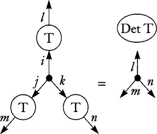
This expression has three free indices, l,m,n, but we can do this one without an array of Polynomials.

Matrix T(“abc”

 “def”

 “ghj”);

forIndex(l)

forIndex(m)

forIndex(n)

{

 Polynomial P;

 forEpsilon(e1)

 {

 int i,j,k;

 int s = epsilon(e1,&i,&j,&k);

 P += s*T(i,l)*T(j,m)*T(k,n);

}

cout <<l<<m<<n<<" "<<P<<endl;

}

This prints the following imposing stuff:

+0+0+0 +0adg

+0+0+1 +0adh+0aeg+0bdg

+0+0+2 +0adj+0afg+0cdg

+0+1+0 +0adh+0aeg+0bdg

+0+1+1 +0aeh+0bdh+0beg

+0+1+2 +1aej−1afh−1bdj+1bfg+1cdh−1ceg

+0+2+0 +0adj+0afg+0cdg

+0+2+1 −1aej+1afh+1bdj−1bfg−1cdh+1ceg

+0+2+2 +0afj+0cdj+0cfg

+1+0+0 +0adh+0aeg+0bdg

+1+0+1 +0aeh+0bdh+0beg

+1+0+2 −1aej+1afh+1bdj−1bfg−1cdh+1ceg

+1+1+0 +0aeh+0bdh+0beg

+1+1+1 +0beh

+1+1+2 +0bej+0bfh+0ceh

+1+2+0 +1aej−1afh−1bdj+1bfg+1cdh−1ceg

+1+2+1 +0bej+0bfh+0ceh

+1+2+2 +0bfj+0cej+0cfh

+2+0+0 +0adj+0afg+0cdg

+2+0+1 +1aej−1afh−1bdj+1bfg+1cdh−1ceg

+2+0+2 +0afj+0cdj+0cfg

+2+1+0 −1aej+1afh+1bdj−1bfg−1cdh+1ceg

+2+1+1 +0bej+0bfh+0ceh

+2+1+2 +Obfj+0cej+0cfh

+2+2+0 +0afj+0cdj+0cfg

+2+2+1 +0bfj+0cej+0cfh

+2+2+2 +0cfj

You can, if you like, make this neater by jiggering the operator < < routine to avoid printing monomials with a coefficient of zero. It's sometimes interesting, though, to see what monomials were added and subtracted (with net coefficient of zero) to an expression.

Some Cubic Identities

The following quantity is identically zero for all values of C:

$Z_l^k={\epsilon }^{ijk}{C}_{ijl}$

In diagram notation,

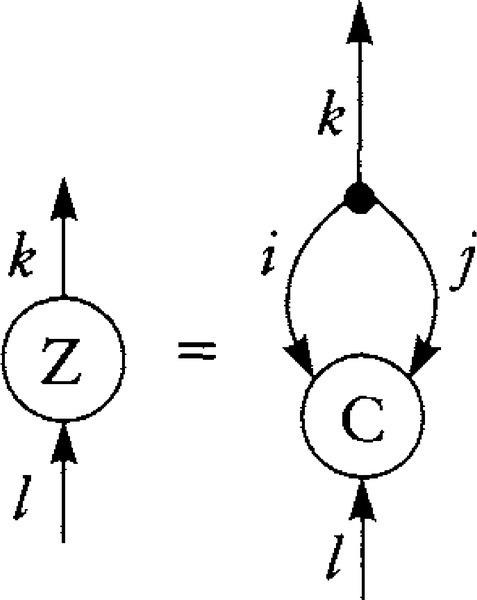
We verify this by

Tensor3 C(“ABE” “BCF” “EFH”

  “BCF” “CDG” “FGJ”

  “EFH” “FGJ” “HJK”);

forIndex(l)

{

 Polynomial Zl[3];

 forEpsilon(e1)

 {

 int i, j, k;

 int s = epsilon(e1,&i,&j,&k);

 Zl[k] += s * C(i,j,l);

 }

 forIndex (k)

 cout <<"Z ("<<l<<k<<") = "<<Zl[k] <<endl;

}

The printout is

Z(+0+0) = + 0F

Z(+0+1) = + 0E

Z(+0+2) = + 0B

Z(+1+0) = + 0G

Z(+1+1) = + 0F

Z(+1+2) = + 0C

Z(+2+0) = + 0J

Z(+2+1) = + 0H

Z(+2+2) = + 0F

This means that if we see such a diagram fragment embedded in a larger diagram, we can immediately say that the whole thing is zero.

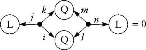
Likewise, the following expression containing a cubic is also identically zero for any tensor C:

${\epsilon }^{ijk}{\epsilon }^{lmn}{\epsilon }^{pqr}{C}_{ilp}{C}_{jmq}{C}_{knr}$

In diagram form,

As code,

Polynomial P;

forEpsilon(e1)

forEpsilon(e2)

forEpsilon(e3)

{

 int i,j,k,   l,m,n,   p,q,r;

 int s = epsilon(e1,&i,&j,&k)

 * epsilon(e2,&l,&m,&n)

 * epsilon(e3,&p,&q,&r);

 P += s*C(i,l,p) *C(j,m,q)*C(k,n,r);

}

cout <<P<<endl;

This prints out

+0ADK+0AGJ+0BCK+0BFJ+0BGH

+0CEJ+0CFH+0DEH+0EFG+0FFF

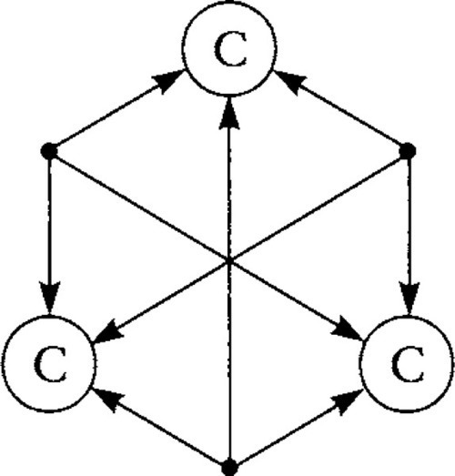
The final example is a bit more complex. We will evaluate the C₄ invariant of a 2DH cubic curve as described in Chapter 20.

${\epsilon }^{ijk}{\epsilon }^{lmn}{\epsilon }^{pqr}{\epsilon }^{tuv}{C}_{nqv}{C}_{jru}{C}_{kmt}{C}_{ilp}$

For fairly obvious reasons, I call it the “cube invariant” because of the diagram

I'm going to do something slightly different this time for the C++ code. All our examples so far have made the code mimic the algebraic expression. This is easy to use, but can be a bit slow. That's because there is a lot of creation, sorting, and destruction of temporary Term variables during execution of the binary multiply operator. I'll write the code for the following example to show an alternative way to generate the Term that uses our existing machinery, but avoids unnecessary creation and deletion.

Polynomial P;

forEpsilon(e1)

forEpsilon(e2)

forEpsilon(e3)

forEpsilon(e4)

{

 int i,j,k, l,m,n, p,q,r, t,u,v;

Term T(epsilon(e1,&i,&j,&k)

  * epsilon(e2, &l, &m, &n)

  * epsilon(e3,&p,&q,&r)

  * epsilon(e4,&t,&u,&v)); // create once

 T *= C(n,q,v);  // modify existing one

 T *= C(j,r,u);

 T *= C(k,m,t);

 T *= C(i,l,p);

 P += T;

}

cout << P << endl;

This generates the following:

+24ACGK−24ACJJ−24ADFK+24ADHJ+24AFGJ

−24AGGH−24BBGK+24BBJJ+24BCFK−24BCHJ

+24BDEK−24BDHH−24BEGJ−48BFFJ+72BFGH

−24CCEK+24CCHH+72CEFJ−24CEGH−48CFFH

−24DEEJ+24DEFH+24EEGG−48EFFG+24FFFF

How Do I Like This?

C++ giveth and C++ taketh away. The internal machinery of the map object keeps its key/value pairs stored in some sort of binary tree thingy so that searching is very fast. This is something I would not have felt like getting into myself. That's good. But the simple mimicking of an algebraic expression by a C++ expression implies a lot of strange jiggery-pokery going on during the creation of a Term. That's not so good. But who cares really. The execution time of the examples shown here is negligible. It's only when you get upwards of eight epsilons that the program takes a noticeable amount of time. Rewriting the expressions as in the final example helps here. For even more complex situations, it would be easy to add an explicit Term constructor that is passed a sign and some fixed number of Symbols. This constructor could resize Monomial once, assign the Symbols to it explicitly, and only need to sort it once. I'll leave that as an exercise for you to do yourselves.

What's next

One can imagine any number of extensions to this code to handle more general expressions. But what we have here is good enough to serve as a check on our theoretical investigations to make sure we don't miss any constant factors or stray minus signs. Now that we can verify some of our computations, we can look for the geometric meaning of transformationally invariant algebraic quantities (invariant because they can be written as tensor diagrams). That will be the topic of future columns.