
The topics in this chapter range from next steps (A* path finding) to topics at the leading edge in game AI (planning, behavior trees). In between is machine learning. All these are of interest to AI programmers and are the subject of articles and even whole sections in the four volumes of the AI Game Programming Wisdom series of books. Besides being the topics of game-industry–focused publications, game AI issues have been picked up by academia as vehicles for research. Game AI is too broad for one book to cover, so we will wrap up with a selection of topics.
This topic might be considered the graduation exercise for the readers of this book. The algorithm is one that all AI programmers need to have mastered. Rather than provide a project with code, just the algorithm is given. Armed with an understanding of how it works and aided by the numerous free resources available on the Internet, you should be able to write your own implementation of A*.
A* (pronounced A-star) is the algorithm of choice for general path finding in most games. Path finding answers the question, “What’s the best way to get from here to there?” If there are only a few places in your game, you can precompute the paths between them and store the paths.
Precomputed paths are cheaper than A* paths, but two major issues crop up quickly. The first issue is that the number of paths explodes as the number of places increases. The number of paths is related to the square of the number of places. The second issue is that precomputed paths require knowing all the places in advance. They cannot be used with dynamically created maps. Precomputed paths fail if elements such as bridges can be rendered unusable during play. When you lack a static map with a small number of places, you need a general path finder, and A* is hard to beat.
A* works with two core concepts. The first is, “I know how much it costs to get from the starting point to here,” for any particular “here” to which the algorithm has progressed. The second concept is, “I can estimate the cost of getting from here to the goal,” again for any particular “here.” In technical terms, A* is a best-first graph search algorithm to determine the lowest cost path between two nodes. We will examine what all these words mean and why they are important.
The best-first part is one of the major reasons why A* is so popular. A* is reasonably fast, and that speed comes from examining the most promising steps first. A character standing in a building would first check if he or she can walk directly toward his or her goal. If the character is standing in an open-air gazebo, this will in fact be the best way to go. If the character is standing in a room with walls and doors, the extremely high cost of going through a wall would force the character to examine less direct paths. If there is a door in the wall blocking the direct path, that door will probably be checked before other doors that lead away from the goal.
“Reasonably fast” is a relative term. A* is a search method, and search as a computational problem is not cheap. The difference between “cheaper than the alternatives” and “cheap” should be kept in mind.
A* is a graph search algorithm. For navigation purposes, most virtual worlds are not really contiguous. Unlike on Earth, in games, the concept of “here” is not a set of coordinates such as latitude and longitude that can always be more finely specified. In games, “here” is some discrete space, perhaps a triangle. Board games often use squares or hexagons for this purpose; they are spaces that cannot be subdivided. Whether in board games or computer games, every “here” has some neighboring places that are directly connected to it. To A*, a graph is a set of points and a set of lines connecting those points to their neighbors. These points represent the “here” for any location in the virtual world; in graph-theory terms, these are called nodes. Every square or hexagon in a board game becomes one node in a graph. The lines connecting the nodes, called edges of the graph, have costs associated with them. A roadmap showing only the distance between cities is a familiar example of this kind of graph; the roads are drawn as simple straight lines, and the cities are drawn as circles. Our discrete computer-game world can be modeled as a graph like this. Outside of navigation, our game may have a very finely detailed and continuous definition, but for navigation purposes there are powerful motivations for minimizing the number of nodes in the graph. A* is going to search for a path through the nodes, and having fewer nodes yields a faster search.
As long as certain givens remain true, A* will produce the lowest-cost path between the two nodes if any legal path exists. So what are the certain givens about A* that need to remain true? The big one is the heuristic upon which A* depends. A* uses a heuristic to make decisions using imperfect data. Perfect data would be expensive to compute, and much of it would be thrown away. The heuristic in A* tells the algorithm that from any point in the graph, the distance to the goal is at least a certain amount. Of the two core concepts in A*, this is the estimate part. For driving on roads, a good heuristic is the direct straight-line overland distance to the goal.
There are two major requirements for a good heuristic. The first is that it needs to be admissible, and the second is that it needs to be as close as possible to the actual distance. An admissible heuristic is one that is never larger than the actual distance.
As an example, imagine that our heuristic was the direct straight-line overland distance. Because driving is restricted to roads, the actual path will generally be longer than the heuristic. But we know that the actual path is rarely shorter (a tunnel through a mountain could be shorter than the direct path over the mountain). If we have no tunnels, the heuristic is admissible; if we have tunnels, the heuristic is inadmissible.
It should be easy to get a heuristic that never overestimates the actual distance between two nodes, but we also want it to be as large as possible without going over. We will see the importance of this when we get to some examples. If the roads are all set on hillsides, none of them will ever be anywhere near as short as a straight line, so we should adjust the heuristic to something larger than the direct distance.
Both parts of a good heuristic have a profound impact on the performance of A*. We can use Figure 10.1 to walk through an example of how A* works.
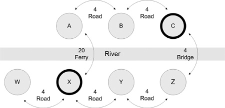
On some major rivers such as the Rhine, there are few bridges and many ferry stops. Let us consider a journey from C to X in Figure 10.1. Presume that all the towns are regularly spaced to make the math simpler. It takes only four minutes to drive on the roads between two neighboring towns, but using the ferry takes 20 minutes. If you could drive it, B and X would be 5.66 minutes apart, taking the diagonal into account.
A* starts at the beginning and evaluates the nodes around it. So if the trip is from C to X, the algorithm starts with C, which has neighbors B and Z. Because we start at node C, the cost to get there is 0. In A* terms, this is g, the known lowest cost to get to a node. This is the first of the core concepts of A*: knowing the actual cost to get someplace. The cost to get to B is 4. Because the bridge and the road are equally fast, the cost g to get to Z is also 4.
Is it faster to take B or Z to get to X? We do not know, but we can use a heuristic to make a guess. In A* terms, the heuristic is h, the estimated cost to the goal. For this example we will use straight-line driving time, which is directly proportional to distance, as our heuristic. Obviously we cannot use the actual driving time; if we do not yet know what the shortest path is, how can we know how long it will take to drive?
The heuristic h tells us that Z is 8 minutes away from X, and using a direct diagonal path, B is 5.66 minutes away from X. Our heuristic is reasonable, but it does mislead us from time to time. No actual cost is lower than our heuristic, a required given if the algorithm is to function optimally. A* uses the sum of the known cost and the estimate of the remaining cost supplied by the heuristic to give f = (g + h), the “fitness” of the node in A* terms. The fitness is used to decide what node to pursue next. This is where the best-first part of the algorithm comes into play; fitness tells us the best node to examine next. Let us examine the values we have so far.
We started with node C, but because it is not the goal and we have added all its neighbors to the list of nodes to examine, we are done with C. After we dealt with node C, we had B and Z to pick from.
Node B: f = g þ h = 4 þ 5.66 = 9.66
Node Z: f = g þ h = 4 þ 8 = 12
At this point, we can offer some commentary on our heuristic. At node B, we estimated 5.66 as the cost to X. The actual value using the ferry is 24. Even if there had been a bridge instead of the ferry, the actual would have been 8. This amount of underestimation is making B look more enticing than it is. We will waste time exploring from B before we decide to abandon it and go through Z.
If we know that our nodes exhibit a regular grid pattern and lack diagonals, we can use the “Manhattan distance” as our heuristic. Instead of using Pythagoras’ theorem to compute the hypotenuse of a right triangle from the lengths of the sides, we simply add the lengths. On the streets of a city with a grid pattern of streets, this is the distance that will be covered to get from one place to another.
In our example, using Manhattan distance makes the estimate for node B equal 8. A larger but admissible estimate makes us more likely to abandon suboptimal nodes earlier, and that is a serious performance gain. In this case, it puts node B and Z on equal footing. Tuning the heuristic to the particulars of the application is an important optimization. Let us return to the algorithm using our original heuristic.
Node B is more promising at this stage, so it will be examined first. We will keep Z around in case B does not work out. Node B is not our destination, so we have to add its neighbors (in this case, just node A) to the list of nodes to examine. We do not add nodes we have already visited, such as node C; driving in circles never makes a path shorter. Getting to node A adds 4 to the known cost to the goal, g, and the estimated cost (h) to get from node A to node X is 4 (because that is the straight-line distance to cross the river).
Node A: f = g þ h = 8 þ 4 = 12
With that, we are done with node B. Nodes A and Z have the same estimated cost, so we could investigate either one next. Since it doesn’t matter which we choose, let’s look at node A next. The only new neighbor to add to our list is node X. Getting from node A to node X costs 20 (since we have to take the ferry), so we add that to 8, the known cost for node A, giving us a g of 28. Since node X is the goal, h is zero.
Node X (via A): f = g þ h = 28 þ 0 = 28
When we compare the 28 to the values we have, we find that we have paths with a potentially lower cost. Node Z is claiming 12 for its estimated total cost. As long as that path can stay under 28, we will continue pursuing it. Going from Z to Y adds 4 to g, the known cost thus far to the goal.
Node Y: f = g þ h = 8 þ 4 = 12
That finishes node Z. The path using node Y is still below our 28, so we continue. Going on to X from Y adds 4 to g, the known cost thus far to the goal. Since X is the goal, we have the following:
Node X (via Y): f = g þ h = 12 þ 0 = 12
There are no paths left that might come in lower, so we have the shortest path. By using best-first, A* can still pursue blind alleys, but it abandons them as soon as their cost rises above alternatives. It does not foresee obstacles, but it will avoid them as they appear.
Implementing A* is harder than understanding how it works. The details in this section will be of particular interest to those readers who will need to implement their own A*. We will go over the lists used to make A* work, and we will comment on how admissibility of the heuristic has a performance impact.
We keep two lists in A*: the open list and the closed list. The open list holds nodes that might need further examination. We need to be able to easily find the node with the best fitness from the open list because that is always the next node to examine. To hold nodes that are no longer on the open list, we have the closed list. Once we have put the neighbors of a node on the open list, we can take that node off the open list and put it on the closed list. The two lists make things easier to juggle.
To start with, we added C to the open list. Each step involves removing the fittest node from the open list and checking its children to see if they get updated and belong on the open list. In the evaluation of node C, we removed C from the open list after we added nodes B and Z to the open list and updated their values. B and Z had not been looked at before, so their values were set, and they went onto the open list. New nodes always go on the open list. Neighboring nodes already on the open list will have their numbers updated only if the new numbers are better. Neighboring nodes on the closed list go back on the open list only if their numbers improve, but this will never happen if the heuristic is good, and the cost always increases with additional steps. Since most applications have the cost increase with each step, the only concern is with the heuristic.
For simplicity, we did not show in the discussion the fact that when we evaluated node B, the algorithm considered going back to node C since node C is a neighbor of node B. Node C was given a 0 value for g when we started. A path that goes from node C to node B back to node C will want to give C a g value of 8, which is worse than what is already there. For path finding related to travel in time or space, the costs always increase, so looping paths will automatically be worse than non-looping paths. C is a neighbor of B, but C will not go back onto the open list unless it can do so with better numbers than it already has. This never happens in our example because cost is monotonic (taking another step can only increase cost) and our heuristic is admissible. Because it never happens, we can safely ignore any neighbor that has made it to the closed list. Real implementations of A* would not have computed the cost of going to node C; instead they would first see if node C was on the closed list, and if it was they would ignore node C.
Being able to ignore nodes on the closed list is a huge performance win! Once again, this optimization is made possible by having an admissible heuristic and monotonically increasing cost. Monotonically increasing cost is usually a given, but admissibility of the heuristic is a design decision.
If the estimate provided by the heuristic is sometimes higher than the actual cost, not only do we no longer have a guarantee that the path we get will be the shortest one, but we may also find that we need to move nodes that are on the closed list back to the open list in pursuit of the shortest path. It is extremely unlikely that any real implementation of A* will ever allow backtracking by reexamining nodes on the closed list.
Let us change our example to see what happens if the heuristic is not always admissible and we still want the shortest path. We will have to take some liberties with the graph to make this happen, yielding the revised graph shown in Figure 10.2. In order to shorten travel times, the cities at node A and node X have commissioned a catapult service to fling travelers across the river extremely quickly. This makes our heuristic inadmissible. The move to catapult service was sparked by heavy rains that forced the cancellation of the ferry service and caused major damage to the road between node B and node C. The roads to and from node X also suffered some minor damage.
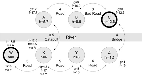
We wish that the code should not need to touch any node that it has already touched, but the combination of an inadmissible heuristic and the desire for the shortest path means we need to handle paths that split and then merge differently than before. If a second path makes it to a merge point—a node we have already touched—with a lower g value than what the merge point already has, then the first path through the merge point is not the optimal path, and the merge point goes back onto the open list with new values for g and f. This is the case in Figure 10.2.
Again, we start at C. Our final goal is node W instead of node X. Node X is the merge point. The numbers for the nodes are shown in the figure. Node C goes on the open list first. Being the only node there, its neighbors, B and Z, which are not on any list, go on the open list, and C goes on the closed list. We examine the open list for the most promising node.
Z at 16 beats B at 16.9, so Z is examined next. Z cannot improve C’s numbers, so C stays on the closed list. Z puts Y on the open list with B because Y is a new node. We are done with Z, so it joins C on the closed list. Again, we examine the open list for the most promising node.
Y at 16 also beats B at 16.9, so we examine Y. Y cannot improve on Z’s numbers, so Z stays on the closed list. X is new, so it goes on the open list. Y is done, so Y joins Z and C on the closed list.
From the open list, B at 16.9 beats X at 17, so we examine B next. B cannot improve C’s numbers, so C stays on the closed list. A is new, so B adds A to the open list with X. B gets put on the closed list with C, Z, and Y.
On the open list, X at 17 beats A at 17.7, so we examine X next. X cannot improve Y’s numbers, so Y stays on the closed list. X cannot improve A’s numbers, so X does not update A on the open list. W is new, so X puts W on the open list. X joins Y, Z, C, and B on the closed list.
On the open list, A at 17.7 beats W at 18, so A is examined next. Here is where we will encounter the effects of an inadmissible heuristic. The catapult method of crossing the river is far faster than the heuristic expects anyone to ever go. This is where the heuristic gives an inadmissible estimate of the cost. Node A cannot improve B’s numbers, so B stays on the closed list. Node A can improve X’s numbers, so X is updated and moved from the closed list back to the open list to join W.
An A* implementation that has the normal optimization of ignoring nodes on the closed list would not have touched X again. Nor would it have taken the effort to see if it could improve the numbers of any node on the closed list as we did in the preceding paragraphs. Node A goes onto the closed list with B, C, Y, and Z.
The open list is again checked. X at 16.5 beats the existing W at 18, so X is given another chance. X cannot improve A or Y, so they remain on the closed list. X can improve W on the open list, so W goes from 18 to 17.5. X goes to the closed list with all the other nodes except W. Since the goal node has the best score on the open list, it is used as it is.
This example shows that the world does not end if the heuristic is sometimes inadmissible. It can have easily happened that with an inadmissible heuristic, A* will not find the shortest path, regardless of whether it reexamines nodes on the closed list or not (see Exercise 2 at the end of this chapter). This is the penalty for using an inadmissible heuristic. But if catapults are rare and roads are the norm, we might stay with our inadmissible heuristic. We do this because it is more aggressive about discarding paths early, and that is a performance win. The effect in our example would be that sometimes, the pathfinder neglects to exploit catapults when they are off the beaten path. In our example, the catapult is 8 times faster than the heuristic. If we tune for catapults instead of roads, we have to expand our searching by a factor of 8 to get to the point where we say, “Even a catapult won’t help you when you are this far away,” and that could be a lot of useless searching.
Since reexamining nodes on the closed list does not guarantee getting the shortest path when the heuristic is inadmissible, and reexamining nodes on the closed list is pointless when the heuristic is admissible, the case for reexamining nodes on the closed list is too weak to justify.
Besides holding the f, g, and h numbers, each node also tracks what node came before it in the path. When our code reached X via A, X would store A. When a node is placed on the open list for the first time or updated with better numbers, the node is also updated with the new predecessor in the path. When our example reached X via Y, it updated the costs and also overwrote the stored A with Y. This way, when A* completes, the nodes have stored the best path.
A* is popular because it usually performs well and gives optimal results. Performing well does not make it free, however; A* can be costly to run. When no path exists, A* exhibits maximum cost as it is forced to explore every node in the graph. If the usual case is that paths usually exist and obstacles are localized, then dealing with the difference in performance between the usual case and the worst case presents a difficult engineering challenge.
A* also depends heavily on the concept of “here” in the graph. The world may be represented at a low level by a mesh of tiny triangles that can be fed to the graphics engine, but that mesh makes for expensive path finding. A room may have a large number of triangles that make up the floor, but for navigation purposes it can be reduced to a single “here” or a small number of “heres.” To help with path finding, many games have a coarse navigation mesh with far fewer nodes than the graphics mesh. The navigation mesh makes the global pathfinder run quickly by greatly reducing the number of nodes. The nodes in the navigation mesh can be forced to have nice properties that make them easier to deal with, such as being convex. Path finding within a node in the navigation mesh is done locally, and simple methods often suffice; if the node is convex, then a straight line is all that is required.
An issue with any pathfinder is that long paths are fragile paths. Bridges get blown up, freeways are subject to being closed by accidents, and fly-over rights can be denied after a flight takes off. Before blindly using A* and expecting all paths to work, you should investigate the methods that are being used to deal with path problems.
Before the novice AI programmer rejoices that path finding is solved, he or she needs to consider the needs of the virtual world. A* will rightly determine that using roads and bridges is better than taking cross-country treks and fording streams. What A* does not do is traffic control. Unexpected traffic jams on popular routes and near choke points are realistic, but so are traffic cops. The game’s AI might be smart enough to prevent gridlock, but the planning code still has a problem. The planning code has to factor in the effects of the very traffic the planning code is dispatching. If the planning code places a farm tractor, a truck carrying troops, and a motorcycle dispatch rider on the same narrow path in that order, the whole convoy is slowed to the speed of the tractor. A* told the planner that the dispatch rider will get to its destination in far less time than will actually happen. A* told the planner that the troops will get there on time as well. Even worse is the case when opposing traffic is dispatched to both sides of a one-lane bridge. A* by itself may not be enough.
Machine learning has been “the next big thing” in game AI for many years. The methods have been described as elegant algorithms searching for a problem to solve. The algorithms have been put to good use in other areas of computer science, but they have gained very little traction in game AI. People have been looking for ways of getting around the limits of machine learning in games for some time now [Kirby04].
Realizing the potential of machine learning is difficult. There are many kinds of machine learning. Two of them are popular discussion topics: neural networks and genetic algorithms. Neural networks appear to be very enticing, particularly to novice game AI programmers. They have been a popular topic for over a decade in the AI roundtables at the Game Developers Conference. The topic is usually raised by those with the least industry experience and quickly put to rest by those with many years of experience. The conventional wisdom is that neural networks are not used in commercial games. By contrast, genetic algorithms have gained a very modest toe-hold into game AI, but not in the manner that you might first expect, as we shall see. A major goal of this section is to give beginning AI programmers sufficient knowledge and willpower to enable them to resist using either method lightly.
Before considering the different machine-learning algorithms, it is worthwhile to consider how they will be used. The first big question to ask of any proposed game feature is, “Does it make the game more fun?” If cool techniques do not translate into improved player experience, they do not belong in the game.
The next big question to answer is, “Will it learn after it leaves the studio?” For most machine learning used in games, the answer is a resounding “No!” Quality-assurance organizations do not want support calls demanding to know why the AI suddenly started cheating or why it suddenly went stupid. In the first case, the AI learned how to defeat the player easily; in the second case, the AI learned something terribly wrong. Most ordinary car drivers are happy with the factory tuning of their real-world automobiles, and most players are fine with carefully tuned AI. That being said, the answer is not always “No”; Black & White is an early example of a game that turned machine learning in the field into a gameplay virtue.
Learning algorithms are susceptible to learning the wrong thing from outlier examples, and people are prone to the same mistake. Black & White learned in the field, and learning supported a core gameplay mechanic. One of the main features of the game was teaching your creature. If teaching is part of the gameplay, then learning is obviously an appropriate algorithm to support the gameplay. How many games can be classified as teaching games? Most games do not employ teaching in their gameplay, and most of those same games have no need of learning algorithms. There may be other gameplay mechanics besides teaching that are a good fit for machine learning in the field, but it will take an innovative game designer backed by a good development team to prove it.
The final question always to ask is, “Is this the right tool for this job?” For neural networks in game AI, the answer is usually an emphatic “No.” In some cases involving genetic algorithms, the answer will be a resounding “Yes.” One of the clarifying questions to ask is, “Is it better to teach this than it is to program it?” Of course, “better” can have many different interpretations: easier to program, produces a better result, can be done faster, etc.
The trick with teaching—or training, as it often is called—is to make sure that the right things are taught. This is not always a given. A system trained to distinguish men from women at first had trouble with long-haired male rock stars. Another image-analysis system learned to distinguish the photographic qualities of the training data instead of differences in the subjects of the photographs. The system is only as good as the training data; it will faithfully reflect any biases in the training data. Lionhead Studios improved the user interface to the learning system in Black & White II to make it explicitly clear to players exactly what feedback they were about to give their creature, solving a major source of frustration with the original game.
The most straightforward way to ensure that learning has taken place is to administer a test with problems that the student has never seen before. This is called an independent test set. A system that is tested using the same data that trained it is subject to memorizing the problems instead of working out the solutions. Just as other software is tested, learning systems need test data that covers a broad range of the typical cases, as well as the borderlines and outliers. The system is proven to work only in the areas that the test set covers. If the system will never encounter a situation outside of the training set, the demand for an independent test set is relaxed.
Hidden in this coverage of training is a fact that needs to be made explicit: We are talking about two different kinds of training. The two methods of training are supervised training and reinforcement training. In supervised training, the learning algorithm is presented with an input situation and the desired outputs. The image-analysis system designed to identify men versus women mentioned earlier was taught this way. The system trained against a set of pictures of people, where each picture was already marked as male or female. Supervised training happens before the system is used and not when the system is in use. If there is a knowledgeable supervisor available at run-time, there is no need for the learning system to begin with. The success of supervised training in learning algorithms outside of the game industry has not been echoed within the game industry. Unless otherwise noted, supervised learning is the default when discussing learning algorithms.
Reinforcement learning, by contrast, emphasizes learning by interacting with the environment. The system starts with some basic knowledge and the need to maximize a reward of some kind. In operation, the system must balance between exploitation and exploration. At any given point in time, the system might pick the action it thinks is best, exploiting the knowledge it already has. Or it can pick a different action to better explore the possibilities. Reinforcement learning uses exploration to improve future decision making by making changes to the basic knowledge the system starts with.
A good introduction to reinforcement learning is given in the first chapter of [Sutton98], which is available in its entirety online. Advanced readers will want to study the method of temporal differences (TD); TD(λ) is of particular interest. Reinforcement learning has produced a few notable success stories; in commercial video games, Black & White used reinforcement learning. TD-Gammon began as a research project at IBM’s Watson Research Center using TD(λ). It plays backgammon at slightly below the skill level of the top human players, and some of its plays have proven superior to the prior conventional wisdom [Tesauro95]. Reinforcement learning creeps into games in small ways as well [Dill10].
Many experienced game AI programmers attribute characteristics of undead vampires to neural networks and genetic algorithms; they are enticing, particularly to the naïve. They keep returning, at least as a topic of conversation, despite heroic efforts to lay them to rest. They cannot be trusted to do what you want them to do, and it takes arcane knowledge and skills to get them to do anything at all. At the end of the project, there is great fear that they will turn to dust should the game ever see the light of day. All kidding aside, what are the real reasons?
There are three basic concerns: control over the AI, lack of past history of achieving a successful AI with these methods in games, and control over the project.
Many game designers demand arbitrary control over what the game AI does. The smarter the AI gets, the more it wants to think for itself. In and of itself, that is not a problem; the problem comes when a designer wants to override the AI, usually for dramatic impact or playability reasons. As we shall see, neural networks effectively are a black box. They might as well carry the standard warning label, “No user-serviceable parts inside.” You can train them (repeatedly if necessary), you can use them, and you can throw them away. For all of the other methods that we have covered in prior chapters, there are places where the AI programmer can intervene. Places where numbers can be altered or scripts can be injected abound in those methods, but not inside these black boxes. They have to be trained to do everything expected of them, and that is often no small task.
Supervised training is notorious for its need of computational resources. In addition, every tweak to the desired outputs is essentially a “do-over” in terms of training. The combination of these two issues is a rather non-agile development cycle. My non-game industry experience with supervised training could be summarized as, “Push the Start Learning button on Monday; come back on Friday to test the results.” When a game designer says, “Make it do this!” the AI programmer starts the entire learning process over from scratch. Worse, there is no guarantee that the system will learn the desired behavior. Nor is there any guarantee that old behaviors will not degrade when the system is taught new ones.
Effectively training a learning system is a black art, and expertise comes mainly through experience. Getting the desired outputs is not always intuitive or obvious. This lack of surety makes the methods a technical risk.
Just as building a learning system is an acquired skill, so is testing one. The learning systems I built were never released for general availability until after they had successfully passed a field trial in the real world. Learning systems in games need their own particular test regimes [Barnes02]. The task is not insurmountable, but it does create project schedule risks—the test team has to learn how to do something new.
The issue of completeness also crops up. A neural network operates as an integrated whole. All of the inputs and desired outputs need to be present to conduct the final training. So the AI cannot be incrementally developed in parallel with everything else. Prior versions may not work in the final game. From a project-management perspective, this is usually unacceptable; it pushes a risky technology out to the end of a project, when there is no time left to develop an alternative if learning does not work out. Good project management calls for mitigating risks as early as possible.
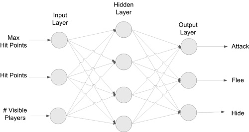
Neural networks loosely mimic the structure of the human brain. As shown in Figure 10.3, a typical network has three layers: the input layer, a hidden layer, and an output layer. The hidden layer helps provide a way to create associations among multiple inputs and multiple outputs. Key to exploiting neural networks is knowing that they are classifiers and that they need the right inputs.
Neural networks are classifiers. They take inputs and render an opinion on what they are. As a learning algorithm, they infer relationships instead of requiring the relationships to be explicitly programmed in. This is critical to understanding the utility of the method. When you know the relationships among the inputs, you can get exactly what you want by directly programming them. When you do not, or when they tend to defy an exact definition, it may be easier and more accurate for the network to infer, or learn the relationship.
At this point, we know enough to ask the final question we should always ask, “Is this the right tool for the job?” If the job of our AI is to classify the situation before it, we might still be okay. However, the job of most game AI is to answer the question, “What should I do?” It is not always obvious that the answer to “What is the situation?” that we get from a classifier will directly yield the answer to “What should I do?” that the AI needs to provide.
The neural network show in Figure 10.3 could be used to determine the best next state in the FSM from Chapter 3, “Finite State Machines (FSMs).” The network classifies the world by indicating the next state that is the best fit to the conditions at hand. Using a neural network for this simple example is total overkill, but recall our discussion of complexity in an FSM. The complexity of the transition rules can be the downfall of an FSM that has a manageable number of states. Using a neural network frees programmers from the task of programming the transition rules, provided they can teach the network instead.
An advantage of using a neural net to classify is that the outputs are not fixed to binary values. In our existing monster FSM AI, when the monster is attacking or fleeing, it has no middle ground in which it is considering both. A neural network can be trained to consider two or more different alternatives. If the training data did not have a sharp cutoff between attacking and fleeing, the neural network will reflect that for those inputs that had more than one different valid output. The training data would indicate that sometimes the monster flees players when hit points are at a given level, and sometimes it continues an attack. The FSM code that disambiguates multiple possible next states can weigh the options presented by the outputs. If the highest output is always used, the behavior will be the same as before. If a weighted random selection is used, the behavior will more closely match the proportions in the training data.
Using a different example, the output of a neural network trained to recognize letters might show strong outputs for Q, G, O, and C when presented with a Q to recognize. If the network did not have a strong preference, the next character might be used to assist in the decision. In English, Q is almost always followed by U or u. Having weighted outputs instead of binary outputs coming from the neural network allows the overall system greater leeway in making decisions. This is true of other methods as well.
Classifiers such as recognition systems are oracles. When asked a question—any question—they give an answer. On the surface this capability seems impressive, but it is also true of the Magic 8-Ball toy. If you feed text that uses the Greek or Cyrillic alphabet to a recognizer trained on the Roman characters present in English, the recognizer will output what it thinks are English characters. It would make the same attempt when fed Hebrew or Hiragana characters or even Kanji symbols and random applications of the spray-paint tool on a bitmap. One of the more important design decisions to make with such a system is what to do when presented with inputs that have no particular correct response. Such inputs are commonly called garbage, but they include ambiguous input as well.
There are two ways to approach this problem. The simplest is to demand, “Give me an answer, even if it’s wrong.” In this case, the system is trained with the broadest array of data available and sent into battle. The alternative is to design a system that has an “I don’t think so” output. In these systems, the training data includes properly marked garbage. Good garbage for training can be hard to find, and tuning systems that have a garbage output can be a black art. The question for the designer is to ponder the difference between an AI that is resolute, if occasionally stupid, compared with one that sometimes does not know what to do. If the designer says, “All the choices are always good, just sometimes some are better than others,” then the resolute system is fine. On the other hand, if there is a good default behavior available to the AI, especially when some of the outputs could be badly inappropriate, then it may be worth the effort to implement a garbage output. Whether it is programmed to recognize garbage or not, a classifier should always be tested with data that has no right answer.
Getting the inputs right can make or break a neural network. The inputs are collectively known as the features presented to the network. We could have pre-processed two of the inputs, hit points and max hit points, and used the ratio as a single input instead. In our particular case, a properly engineered network will infer the relationship, but this is not always a given.
Consider a monster that is in combat with a powerful foe. The monster is losing hit points in large chunks. The monster will go from the attacking state to dead without ever having a chance to flee. Our current set of features is not sufficient. If we add rate of change of hit points as an input feature, our monster can act more intelligently. It can know that it can stay in combat longer against a weak foe, even if the monster is hurting. And it will know to flee early if it is being hammered by a potent foe.
Getting the features right is critical if the network needs to deal with time-varying data. The rate of change in a value (the first derivative, in mathematical terms) can be very useful, as we saw in the monster-hit-points example. The rate of change of a first derivative (the second derivative of the value) can be useful as well. When the steering wheel of a car is turned, the car begins to deviate from a straight course and to rotate. The change rate of the vehicle’s heading (the first derivative) gives a sense of how fast the vehicle is getting around the corner. The second derivative, combined with other data (notably the position of the steering wheel and its first derivative), tells the driver if he or she has exceeded the available traction and is beginning to spin out. The increasing rate of heading change, easily noticed when the second derivative is positive, means that the car is not only cornering, but spinning as well. Stable cornering has a constant rate of change in heading and therefore a zero second derivative (the rate of change of a constant is zero). The amount of counter-steering required to catch the spin depends on how bad the spin is; the second derivative is a very useful number.
Going the other way and summing data over time may also have merit. If the monster is tracking the cumulative number of points of damage it is dealing out to a foe, the monster may have a good idea of how soon it will vanquish a foe without resorting to cheating and looking at the foe’s actual hit points. The monster is guessing at the number of hit points the foe started with, but it will know the cumulative number of hit points that the foe has lost. The cumulative sum is the first integral of damage delivered. The monster may want to decide to stay in a difficult combat because it thinks it can finish off a potent foe before the foe can return the favor. A single value for damage delivered does not tell enough of the story to be useful. Time-varying data typically needs special handling to create effective features to input to a neural network.
As mentioned earlier, using a neural network in place of our familiar monster FSM is total overkill. It is used as a familiar example only. There are better ways than neural networks to do everything we have illustrated so far.
Genetic algorithms are rarely if ever used for game AI. Instead they are sometimes used for tuning variables in games. Motorsports provide us with a good example [Biasillo02]. A mechanic setting up a car manages many tunable parameters to obtain optimum performance on any particular track. There are the camber, caster, and toe angles to be adjusted when doing a basic wheel alignment. There is the braking proportion between front and rear tires—a setting more easily understood if you consider the rear braking needs of an empty pickup truck compared to a fully loaded one. An empty pickup truck needs minimal rear braking force because the lightly loaded rear tires provide minimal traction. A heavily loaded truck benefits from having a great deal of rear braking force to exploit the greater traction available. This is only a partial list of tuning parameters; as you might expect, there can be interactions between variables.
Genetic algorithms can help us in our search for the optimal settings. Genetic algorithms roughly mimic biological evolution. We start with a population that has different characteristics. Some are more fit than others. Cross-breeding and mutation yield new members with different characteristics. Some of these will hopefully be more fit than any of their parents. The best are emphasized for further improvement, possibly along with a small number of less-fit individuals in order to keep the diversity of the population high. The best need not be restricted to children of the current generation; it could include members from older generations as well. We continue until we have a good reason to stop. Let us expand on the concepts of this paragraph in detail.
In programming terms, our variables to tune are the characteristics of our individuals. Each of the angles used in wheel alignment is a characteristic. The braking proportion is another. For production vehicles, you might think that these values have already been optimized by the factory, but the factory settings may degrade lap times to decrease tire wear or increase stability. Even relatively uncompromising road-legal sports cars such as the Lotus Elise are specified for road use and need to be tuned for optimal track handling; specialized vehicles also offer room for improvement on the track.
Selection requires a way to tell which individual is more fit than another. At first blush, we can pick lap time as the fitness function. Why would lap time not be the best fitness function? Most races run more than one lap. One of the compromises in street specifications for wheel alignment is a trade-off between handling and tire wear. Do racers care about tire wear? Racers care about the lowest total time to complete the race (or the farthest distance traveled in a given time period in endurance racing). There is more to it than stringing together a sequence of fast laps. Time spent changing tires might or might not have an impact. Autocross racers have trouble keeping their tires warm between runs and might not wear out a fresh set of tires in an entire day’s competition. Things are very different in NASCAR, especially at tire-hungry tracks such as Talladega. The point is that great care must be taken in selecting a fitness function for a genetic algorithm, or your system will tune for the wrong situation. In motorsports games, as in real life, vehicles are often tuned to individual tracks.
Hidden in the selection criteria is the cost of the fitness function. In our motorsports case, we have to simulate a lap or possibly an entire race with each member of the new population that we want to evaluate. In our case, not only do we have to run a simulated race, but we need a good driver AI. We are going to optimize the car not only for a particular track but also for a particular driver. The cost to mix and match characteristics is typically quite modest when compared to the cost to evaluate them. Not only do we have to select for the right thing, but the very act of measuring for selection must have a reasonable cost.
Crossbreeding in a genetic algorithm involves how we select which parent provides each characteristic of the child. There are a number ways to make the selection, but it is worth emphasizing that the process is selection, not averaging. The child car will not have the toe angle set to the average of the two parents; it will get the exact toe angle value from one of them.
Mutation calls for changing a value in a child randomly to something other than the two values present in the parents. At first glance, it may seem that if the starting population is diverse enough, there is no need for mutation. However, the selection process will tend to suppress diversity as it emphasizes fit individuals who are likely to resemble each other. Diversity is required to keep the algorithm from falsely converging early on a sub-optimal solution.
If we are to keep our population from growing without bound, we need to figure out which individuals are not going to make it to the next run. An obvious method is to replace the worst individuals. Another method would be to replace the members who score closest to the new individuals. Doing selection this way also helps keep a diverse population.
There are many reasons for stopping the algorithm. If the new generations have stopped improving, then perhaps the optimal population has been found, and there is no reason to continue. If the latest generation has individuals that are “good enough,” then it may be time to go on to other things. If each generation takes a large amount of computation, time will be a limiting factor. And finally, if the original population contains individuals thought to be optimal, a few generations may be all that is needed to confirm their status.
Genetic algorithms are good at getting close to an optimal solution, but they can be very slow to converge on the most optimal solution. If the problem can be expressed in terms of genes and fitness, the algorithm gives us a way to search arbitrarily complex spaces. It does not need heuristics to guide it or any expertise in the area searched. Our search speed will depend heavily on how expensive our fitness function is to run.
Behavior trees made it on to the industry’s radar in a big way with Damian Isla’s paper at the 2005 Game Developers Conference [Isla 2005]. The paper was about managing complexity in the AI. Behavior trees bring welcome relief to that problem area without introducing any new major problems of their own.
One of the drawbacks of an FSM is that the number of possible transitions between states grows with the square of the number of states. An FSM with a large-but-manageable number of states may find itself with an unmanageable number of transitions. In Chapter 3, we brushed on hierarchical state machines as a way to control state explosion, with the idea that two-level machines often suffice. If we emphasize the hierarchy more than the state machines, we wind up with something like behavior trees. Behavior trees attempt to capture the clarity of FSMs while reducing their complexity. Behavior trees have been used effectively in some very popular games. Figure 10.4 shows a subset of the behavior tree for Halo 2, and Figure 10.5 shows a subset of the behavior tree used in Spore.
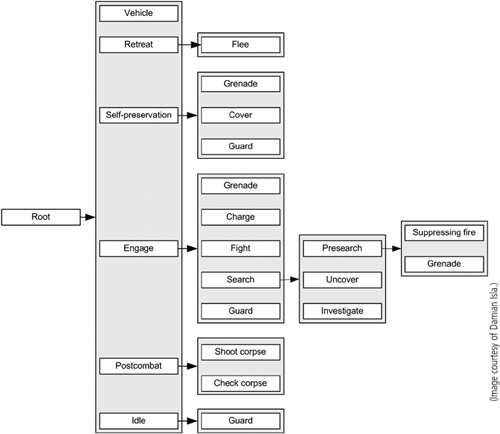
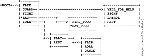
There are a few important observations to make about the trees. The first observation is that the number of levels in the tree is arbitrary. The second observation is that the tree is not a proper tree in that children can have more than one parent. The careful eye will note that Grenade appears in many places in the Halo 2 tree. REST and FIGHT appear more than once in the Spore tree. These are not different behaviors with the same name; they are the same behaviors with multiple parents in the tree. The third and less obvious observation is that there are no loops in the trees. A final observation is that these diagrams are far easier to understand than an equivalent single-level FSM diagram would be. Behavior trees attempt to keep the best parts of an FSM while managing their drawbacks. We will look at how behavior trees work by looking at the two ways we can evaluate them: top-down and bottom-up.
So how do behavior trees work? The Spore behavior tree in Figure 10.5 is marked with asterisks to denote the current state of the AI, which is EAT_FOOD. Each time the AI is asked to think, it starts at the top of the tree and checks that the current decision is still a good one. A common arrangement for the items at any level is a prioritized list. Note that IDLE is listed last on both diagrams. All the ways of disambiguating states can come into play here. All the states have a decider that indicates if it wants to activate and possibly how strongly it wants to activate. So in the Spore case, FLEE, GUARD, and FIGHT can interrupt EAT. If any of them do want to interrupt, the machine has EAT_FOOD terminate, then EAT is asked to terminate, and then the new sequence is started. With no interruptions at the highest level, EAT continues to run. FIND_FOOD has priority over EAT_FOOD, so it can interrupt EAT_FOOD if it wants in the next level down.
Actual implementations of behavior trees include some subtleties. A number of good ideas from other AI methods find a home in behavior trees as well. The current behavior gets a boost in priority when it is rechecked against alternatives. This helps stop the AI from equivocating between two actions. In actual use, the trees need some help to better deal with events in the world. The sound of a gunshot is an event; it is highly unlikely that the AI will ever “hear” a gunshot by examining the current world state. Instead, the event has to be handled immediately or remembered until the next time the AI thinks, and the behavior tree needs hooks to make that memory happen.
An important subtlety more particular to top-down evaluation in behavior trees is that a high-level behavior cannot decide that it wants to activate unless it knows that at least one of its children will also want to activate. In real life, it is wasted effort to drive into the parking lot of a restaurant if no one in the car wants to eat there. This requirement needs to hold true all the way down the tree to the level of at least one usable behavior. The lowest-level items in the tree that actually do something are the behaviors, and all the things above them are deciders. Deciders need to be fast because they are checked often. The Spore diagram only shows deciders. Most of the nodes in the tree we have covered so far do selection; they pick a single child to run. Nodes can also do sequencing, where they run each child in turn.
If there is sufficient CPU available, we can switch from the top-down evaluation described to a bottom-up evaluation. The top-down method requires the highest-level deciders to accurately predict whether any of their descendants wants to activate in the current situation. This capability is critical. Given that assurance, the tree evaluates very quickly, and top-down evaluation gives better performance. Bottom-up evaluation starts by having the lowest-level leaves of the tree, the behaviors, comment on the current situation and feed their opinions up the tree to the deciders. The deciders no longer have to predict whether one of their descendant behaviors wants to activate; instead, they are armed with sure knowledge that includes how much each descendant wants to activate. The deciders are then left with the task of prioritizing the available options. The results are fed up the tree to the highest level for final selection.
What benefit does bottom-up evaluation provide that is worth the performance hit? Bottom-up offers the possibility of better decision making. In particular, nuanced and subtle differences in behaviors can be more easily exhibited in a bottom-up system. The highest-level deciders in a top-down system need to be simple in order to run quickly and to keep complexities from the lowest levels from creeping up throughout the tree. The high-level deciders in top-down make broad-brush, sweeping, categorical decisions. The tree in Figure 10.5 decides between flee, guard, fight, eat, or idle at the highest level before it decides how it will implement the selected category of action. It decides what to do before it works out how to do it. With a bottom-up system, we can let the question of how we do something drive the decision whether to do it. Let us consider an example of how this might work.
In a fantasy setting, an AI character is being driven by the decision tree shown in Figure 10.6. Decider nodes have italic text, and behavior nodes have bold text. Extraneous nodes have been left out for clarity. A top-down evaluation decides to evade at the highest level. The next level down, it has to decide between running away and hiding. It decides to hide in a nearby building, simplified as the Hide node in Figure 10.06 The next level down, it decides between picking the lock on the door, using a spell to unlock the door, or breaking the door down. If the character has no picks and no spells, the only option is to break the door down. Unfortunately, breaking the door down will be obvious to any pursuers. It would be better to keep running away in this case, but the decision between running and hiding has already been made at a higher level, and hiding is usually better than running. Hiding would have been the best choice if the character had picks or a spell.
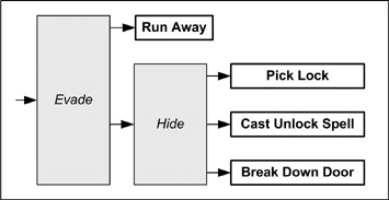
A bottom-up evaluation takes care of this problem. Both the Pick Lock behavior and the Cast Unlock Spell behavior return a very strong desire to activate if the character is properly equipped and no desire at all to activate otherwise. The Break Down Door behavior always returns a weak desire to activate. The Run Away behavior returns a medium desire to activate. The Hide node will pick the best of the three methods for opening the door and offer them to the Evade node in the next level up in the tree. The selected hiding result will be compared to running away. If the character is properly equipped, hiding will be preferred to running away. If the character lacks picks or spells, the character runs away.
Looking at all the leaves this way may seem vaguely familiar. Bottom-up evaluation in a behavior tree is analogous to a rule-based system with an explicit hierarchical disambiguation system. The argument for or against bottom-up evaluation centers on whether or not nuances are lost by making high-level decisions first. If there are no nuances to lose, top-down evaluation is simple and fast. If low-level complexities keep creeping into the high-level deciders, the system is losing the simplicity and possibly the speed that top-down systems are supposed to deliver. In such a case, the system can be simplified by pushing the detail back down to the leaves where it belongs and evaluating from the bottom up.
Behavior trees provide two major advantages: They are easy to understand, and they allow for sophisticated behavior selection. The diagrams shown are easy for AI programmers to understand, and they are easy for experienced game designers to understand. This point is critical; if the vision of the designer is to make it into the AI of the game, the designer needs to understand what the AI will do. Besides being easy for a designer to understand, the diagrams are straightforward for an AI programmer to implement. The method is also easy to debug. All these advantages make for a more productive team, allowing more time to get the AI right because of the clarity provided.
Where does that clarity come from? The diagram partitions the AI problem, allowing the team to look at one node (along with its parents and children) and safely ignore details that are important only to other nodes. FSMs also divide the AI problem, but behavior trees add their hierarchy as an additional way of partitioning the problem that FSMs lack. Hierarchical FSMs are a middle ground between pure FSMs and behavior trees in terms of partitioning. With FSMs, the mindset at any level is finishing the statement, “I am...” yielding a flat diagram. In contrast, a typical behavior tree works on the idea of “The big decisions count the most,” yielding an appropriate number of levels in the diagram. In an FSM, the partitioning is done once; in a behavior tree, it is done as many times as needed. Superior partitioning localizes concerns better. Graphically, this can be seen if the nodes in a behavior tree have few links and the states in an FSM have many transitions. In addition, behavior trees do not loop.
Like all divide-and-conquer methods, great pains must be taken in the divide. If the divide is not clean, then the conquer is unlikely to succeed. The divide step is also a good time to evaluate which method to use. If your tree has minimal levels and a relatively broad base, an FSM or a hierarchical FSM might be the optimal solution. If your tree has much depth or is uneven, with broad parts here and deep parts there, a behavior tree may be best.
Throughout the discussion, we have tied behavior trees to diagrams. Non-graphical methods of specifying a tree or an FSM may detract from the clarity of the design, but decisions about what AI algorithm you use should be made holistically. Tool support may have a strong influence on those decisions; the Spore developers described their particular way of defining their behavior tree as “fairly self-documenting” while at the same time having “the side benefit of compiling extremely rapidly” [Hecker07]. Implicit in that statement is the idea that their design definition was used to generate code, avoiding any disconnect between the design and the code at the potential price of a design that was harder for people to deal with.
The sophisticated behavior selection available does a very good job at handling AI that thinks in terms of “What should I be doing right now?” Whether we evaluate in the typical top-down or the more expensive bottom-up sequence, we arrive at a single thing that the AI should be doing. This is predicated on a fundamental question to ask before considering a behavior tree for your AI: “Can I make high-level decisions or categorizations at all?” Along with that is the question of whether doing just one thing is appropriate.
The benefits to behavior trees come from the fact that they control complexity. If your tree starts with a single root and then explodes immediately into a large number of leaves, you have lost the simplifying power of the method. Put another way, you need to ask, “Can I effectively organize the AI behaviors into a hierarchy?” If there is no benefit to the hierarchy, perhaps another method would be better. If you cannot because you need to string a bunch of behaviors together, a planning architecture may be what you need.
“Can’t the AI just work out all of the steps it needs to pull this off by itself?” is the essential question that brings us to planning. We got a taste of planning in Chapter 6, “Look-Ahead: The First Step of Planning.” In general terms, our AI searched for things to do that would take it to some goal. The preceding sentence seems pretty innocuous, but if we analyze it in careful detail, we can examine any planning system.
Note that we used the term search. Recall the astronomical numbers we computed in Chapters 6, “Look-Ahead: The First Step of Planning,” and 7, “Book of Moves.” Planners do searching as well, so it should come as no surprise that their computational complexity is a serious issue. Writing a planner is no small task, either, but their novel capability of sequencing steps together at run-time make them well worth examining.
You may recall from Chapter 6 that systems that think about the future need a way to represent knowledge that is independent from the game world. This is especially true for planning systems. Good knowledge representation needs to be designed in from the start. The AI is not allowed to change the world merely by thinking about the world; it can only change the world by acting on the world.
Planning AI emphasizes capability instead of action. The elements in a planning system are couched in terms of their results on the world instead of the actions they will perform. Planning elements declare, “This is what I make happen,” instead of emphasizing procedure by saying, “This is what I do.” They are declarative instead of procedural. The overall system is tasked with meeting goals instead of performing actions. With planning, the system is given a goal and given the command, “Make it so” instead of telling all the elements what they are supposed to do.
Consider a visitor to a large city who is talking with friends, some old and some recently met. “I need a place to sleep,” the visitor says. This is declarative. “You can sleep on my sofa,” one friend says, which is the only thing the visitor was expecting. “You can sleep on the other half of my king-sized bed,” another friend offers. “I’m the night manager of a hotel; I can get you a room at cost,” says a third. None of the other friends speak up. All three options meet the goal, and two of them were unexpected. The visitor decides the best plan. The visitor could have said, “Can I sleep on your sofa?” to the one friend and left it at that. This is procedural. While planners deal with dynamic situations gracefully, other, cheaper methods do as well. Planners’ strong suit is more than just picking the single best action.
The biggest benefit of planning comes when the AI assembles multiple actions into a plan. This capability is a reasonable working definition for a planner and the biggest reason to justify their costs. Planning systems search the space of available actions for a path through them that changes the state of the world to match the goal state. Let us look at an example, loosely based on the old children’s folk song, “There’s a Hole in the Bucket.”
The setting is a farm back in the days when “running water” meant someone running out to the well to get water. Our agent, named Henry, is tasked with fetching water. So the goal is to deliver water to the house. There are many objects available for Henry to use, including a bucket with a hole in it. Henry searches for a way to achieve the goal with the objects at hand. He will patch the bucket with straw. The straw needs to be cut to length. He will cut the straw with a knife. The knife needs to be sharpened. He will sharpen the knife on a stone. At this point, we will depart from the song, because in the song you need water in order to sharpen the knife on the stone, and as programmers we despise infinite loops. In our example, the stone will be perfectly fine for sharpening the knife. Our Henry’s plan goes like this: Sharpen the knife on the stone. Cut the straw to fit. Patch the bucket with the cut straw. Use the bucket to fetch water.
Just as behavior trees scale better than pure FSMs, planning systems scale better than behavior trees when the need is for sequences of actions. In a behavior tree, the sequences are assembled by the programmer as part of the tree. With a planner, the AI dynamically performs the assembly, although not without cost. Once again, we see an almost Zen-like condition where adding sophistication makes the systems simpler. The execution systems are becoming more abstract and more data driven. This pulls the actions code into smaller, more independent chunks. What used to be code is slowly turning into something more like data. This phenomenon is not restricted to AI; it is a common progression seen in nearly all programming areas. The cost we mentioned was further alluded to when we said, “adding sophistication.”
By analogy, consider simple programs that use numbers and strings as input data. By now, every reader of this book has written some of them. Consider the task of writing a compiler, such as the VB compiler we have been using. While at the lowest level the input data to the VB compiler is still simple strings, in reality that data is written at a much higher level. The VB compiler as a program is far more sophisticated than nearly all of the programs it compiles. The output of the VB compiler is far more flexible and wider ranging than the simpler programs it usually compiles. Few of the readers of this book are sufficiently qualified to write a VB compiler. “Adding sophistication” raises the bar for the programmers. We need not debate whether writing a planner is more or less difficult than writing a compiler, but we should again also emphasize that the more-sophisticated programs consume more-sophisticated data. VB code is more than simple strings, and the actions made available to a planner are likewise more than simple strings.
We will examine three planning systems: STRIPS, GOAP, and HTN. The latter two (along with behavior trees) are very current topics among industry professionals.
STRIPS stands for the Stanford Research Institute Problem Solver and dates to 1971 [Fikes71]. The basic building blocks in STRIPS are actions and states. From these, we can develop plans to reach goals. Let us examine these states, goals, actions, and plans. Along the way, we will touch on conditions as well.
States are not the states of an FSM, but the state of the virtual world. States can be partial subsets of the world state. States in this sense are a collection of attributes that have specific values. A state for nice weather might call for clear skies and warm temperatures.
Goals are specified as states in this manner. A goal state is defined by a set of conditions that are met when the goal is reached. Goal states differ from other states in that the AI places importance on achieving the goal states, and it does not particularly care about other states along the way to the goal.
Actions have preconditions and postconditions. An action cannot be performed unless all its preconditions are met. If an action succeeds, all the postconditions of the action will become true, whether they were previously true or not. As far as the planner is concerned, only things expressed in the preconditions or postconditions matter. Planners are results oriented.
Let us examine the sharpen knife action from Henry’s plan to mend the bucket earlier in this section. It would have two preconditions: Henry has to possess the knife, and he has to possess the stone. As a postcondition of the action, the knife will be sharp.
A plan is a sequence of actions leading to a goal. Every precondition of every action that is not forced to be true by a prior action in the plan must be true in the initial state that is used to develop the plan. If those conditions are true and the plan is successfully executed, then the world state will match the goal state at the end.
Let us revisit our example of Henry and the bucket. Our states are given in Table 10.1. We have two states of interest: the state of the world and our goal state. The goal state only has one condition: showing that most states are far simpler than the world state.
Table 10.1. Hole-in-the-Bucket States
State | Conditions |
|---|---|
World | Kitchen has no water. |
Bucket has a hole. | |
Have straw. | |
Straw is too long. | |
Have a knife. | |
Knife is dull. | |
Have a stone. | |
Goal | Kitchen has water. |
To transform the world state so that it also matches the goal state, we have the actions listed in Table 10.2. The column order shows how the action transforms the state of the world; start with the preconditions and perform the action to get the postconditions.
Table 10.2. Hole-in-the-Bucket Actions
Precondition | Action | Postcondition |
|---|---|---|
Bucket is mended | Use bucket | Water is delivered. |
Cut straw is available | Mend bucket with straw | Bucket is mended. |
Have a knife | ||
Have straw | ||
Knife is sharp | Cut straw to length | Cut straw is available. |
Have a stone | ||
Have a knife | Sharpen knife | Knife is sharp. |
We start with the goal. The only action that transforms the world state to the goal state is the “use bucket” action. The precondition for using the bucket is not met, so we seek actions that will transform the world state to one where the preconditions are met.
The mend the bucket action has the postcondition of the bucket being mended, which meets the preconditions needed for using the bucket. This might not be the first time that the bucket needed to be mended. If the world state had included leftover straw from the last time the bucket was mended, all of the outstanding preconditions would be met, and we would get a shorter plan that used the state of the world instead of more actions. In our case, we do not have cut straw.
The cut straw to length action has that as a postcondition. To make use of this action, we need to meet three preconditions. The state of the world provides us with a knife and with straw meeting two of the preconditions, but the knife is dull, giving our plan another outstanding precondition. If we cannot find a way to meet this outstanding precondition, this particular plan will fail.
The sharpen knife action can meet the outstanding precondition, but it adds two preconditions of its own. The world state provides both the knife and the stone, meeting all of our outstanding preconditions. This leaves us with a workable plan; the world state, when transformed by a string of actions, meets the goal state.
Our simple example illustrates chaining actions together into a plan but leaves out dealing with alternatives and failures. We might also have scissors capable of cutting the straw but lack a sharpening stone. As you might expect, an initial plan to use the knife would fail to meet all of its outstanding preconditions, and the planner would explore using the scissors instead. We will see these facets of planning in the sections on GOAP and HTN planners.
The ideas behind STRIPS are reasonably easy to grasp. The complexities of programming the system are not trivial. A great deal of effort needs to be applied to the knowledge-representation problem presented by states, preconditions, and postconditions. The knowledge-representation issues have implications about the interface between the planning system and the game. STRIPS is not widely used in games.
If Damian Isla’s presentation on behavior trees at the 2005 Game Developers Conference put that method on the radar of game AI programmers, then Jeff Orkin’s articles and presentations did the same thing for goal-oriented action planning (GOAP) [Orkin03], [Orkin06]. For our purposes, GOAP (rhymes with soap) can roughly be considered as STRIPS adapted to games and uses the same vocabulary. We will look at how GOAP is typically applied to games.
When used in games, actors controlled by GOAP systems typically have multiple goals, but only one goal active at a time. The active goal is the highest-priority goal that has a valid plan. For independent agents, this single mindedness is not a major drawback. Some games require that multiple goals be active at the same time. In this case, the planner needs to be more sophisticated. It may want to accept a higher-cost plan for one goal so that other goals can be pursued in parallel. It may need to ensure that the many plans have no resource-contention problems. It is up to the game designer to decide whether the game is better served by having a wise AI that plans around these issues or a potentially more realistic AI that correctly models the problems. Adding such a capability adds complexity to an already complex algorithm, and it adds CPU demands to an algorithm that is already demanding of uncomfortable amounts of processing power.
Note
These are real-world problems; a full-scale review by the U.S. military many years ago found that in one scenario, the combined demands of the worldwide commands collectively called for five times the total airlift capacity of the Military Airlift Command and deployment of the Rapid Deployment Force simultaneously to 10 different locations.
In games, GOAP actions are typically simplified so that each action can report a cost value associated with it that can be used to compare that action to other actions. These costs can be used to tune the AI’s preference of one action over another. The lowest-cost action might have a cost of 1. If costs tend to be roughly comparable, the planner will prefer plans with fewer steps. It will accept Rube-Goldberg–style plans only when there are no simpler means of accomplishing the goal. The actions themselves are implemented with scripts or small FSMs that are restricted to doing just the one action. FSMs work quite well because the implementation of the action is often heavily tied to animation sequences, and those sequences are often easily controlled by FSMs.
Given those simplifications to the actions, GOAP planners in games can use the now-familiar A* algorithm to search the action space for a path between the goal and the current state. With A*, the direction in which we search has an impact. To use A* at all, we need a heuristic. We will examine both of these facets in detail.
Note the direction of search, from the goal to the current state. This is for performance reasons. As long as A* has a good heuristic, it will find the lowest-cost path, but the performance will vary, depending on which end of the final path the search starts. The typical GOAP or STRIPS case gives the actor many possible actions that might be checked if we start by acting on the current state. Most of those actions will not take us closer to our goal, which gives us a large search space to examine and discard. If we start at the goal, we are far more likely to see only a few actions that need to be searched to take us toward the current state. As Figure 10.7 suggests, if you start at the base of a tree looking for an ant that is on the tip of one of the leaves, it would be easier for the ant to find you at the base of the tree than it will be for you to find the ant.

If all the actions are simple enough that each one changes only a single postcondition, then we can create a good heuristic for A* to use when estimating. That heuristic is that the minimum cost to finish A* from any point is the number of conditions that need to change. If the minimum cost of a step is 1 and the actions can change only one condition, this heuristic holds true. Plans could cost more if the designer gave some steps higher weight than the minimum to help steer the search. Plans could also cost more if there are no direct paths. Indirect paths happen when the steps that lead to the goal add extra unmet conditions that will need to be satisfied by later actions. A real-world example might be in order.
A farmer who stands at the door of his house wants to go out into the night to find out what is making noise in the barn. A single action, “GOTO,” would take him to the barn. That action has a precondition, “has light to see by,” that is unmet. The lantern has the capability to change that condition, but it also has preconditions for being in hand, for fuel, and for being lit. Since the lantern has fuel, the precondition for fuel does not count. The precondition of being lit does count because the lantern in not currently lit. The matches have the capability to light things on fire, and they carry the precondition of being in hand. So the final plan will have grown to get matches, get the lantern, light a match, light the lantern, and finally go to the barn. The designer might have included a flashlight object that has a much lower cost than the lantern, making it preferable because a dropped flashlight is less likely to cause a barn fire than a dropped lantern. In this case, the flashlight has no batteries, and there are no batteries in the house, so the A* stopped progress on the path using the flashlight when it hit the high cost of driving into town to get more batteries.
A* connected the dots to form a plan to meet the goal. The AI programmer did not have to do it himself or herself the way he or she would have for an FSM. The programming paradigm shifts to something like, “Toss in capabilities in the form of actions and stir them with goals to see what plans you get.” The simplicity of the actions is supposed to make programming the set of them simpler in total than trying to program the equivalent capability in an FSM or a behavior tree.
Knowledge representation is critical to the success of the method. The actions have to be able to get all the inputs they need from the state representation and make concrete changes to it. Notice that many of our preconditions and postconditions are simple Booleans that can be represented by one bit of a bit field. Performance of the knowledge representation is critical, and bit fields are a common way to help achieve it. Goal-oriented agents coded this way resemble goal-driven people; they do not stop to smell the flowers along the way, but they do get the details right.
“Don’t we have a plan for that? Or something close?” One of the caveats that we gave about A* is that although we appreciate its performance, we know it is not free. A* connects the dots for us in GOAP. Maybe there is a way to save and reuse chunks of plans the way we might pre-compute popular paths. Each of the travelers who passed through the Cumberland Gap or crossed the Rocky Mountains on the various trails did not come up with a brand-new plan before setting out (with the possible exception of the disastrous Donner party). We might like our AI to have a deep bag of tricks to use in terms of pre-computed plans while still being able to re-plan when things go decidedly wrong.
At the lowest level, a hierarchical task network (HTN) resembles the other planners we have mentioned. We have actions that can be directly executed if their preconditions are met, providing us with a change to the state of the world. These are often referred to as primitive tasks. HTNs also include a task library. Any task that is not a directly executable primitive task is called an abstract task. The abstract tasks in the task library decompose into lower-level abstract tasks and finally into primitive tasks. An example might be in order.
As shown in Figure 10.8, our farmer from the GOAP example has a “light source” abstract task in his task library. That task decomposes into the “use lantern” and “use flashlight” abstract tasks. The “use lantern” abstract task decomposes into a “light lantern” abstract task and the highly useful “get” abstract task. As they must, all the remaining abstract tasks similarly reduce to primitive tasks, although for simplicity, the diagram does not show the full decomposition of everything. Details of the flashlight and other methods for making fire are not shown.
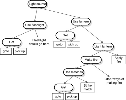
The decompositions are hierarchical. In a rich environment, there will be many such decompositions to choose from for each task; our farmer has a flashlight and a lantern at his disposal for use as a light source, and probably more than one means of making fire. The task library is comparable to a rich script library [Kelly07] and can be computed offline [Kelly08]. There are some compelling advantages to HTN: The plans can be rapidly forward searched, and they deal gracefully with changing conditions. While they can be computed offline, designers can create plans to their liking as well.
The highest-level abstract tasks tend to be a very close match to typical goals that might be presented to a STRIPS or GOAP planner. Instead of running A* from the end goal back to the current state, we can more rapidly find matching high-level abstract tasks that take us to our goal, a welcome performance improvement. Instead of hoping that the ant on the leaf finds us at the base of the tree, we pull out the closest thing we have to an ant-locator plan and follow it directly to the ant. The forward search with HTN is faster than the backward search with GOAP.
Because of their forward and hierarchical nature, HTNs are also part of plan execution. Again using our farmer example, suppose the farmer starts to use the flashlight, and the batteries fail before he gets out the door. The light source task needs to re-plan, but nothing higher in the hierarchy has to change. The basic plan for getting to the barn and exploring the noises is sound. Only the part about getting some light has to change. A GOAP or STRIPS planner would have to restart the search because its plans do not natively retain the dependencies explicitly or keep alternatives that were discarded along the way. Once a GOAP or STRIPS planner discovers the flashlight in our example, it will discard using the lantern. Even if a clever implementation were to recognize that only a portion of the plan had failed, GOAP or STRIPS would need to search through all actions for alternative means of making light. The HTN planner in Figure 10.8 has the alternative light sources encoded in the abstract tasks.
To make sure everything works properly, HTNs include a new feature known as critics. Critics detect conflicts early in an effort to minimize backtracking. Instead of going out to investigate noises in the barn, suppose our farmer was going out after dark to light a bonfire for roasting marshmallows. Critics would detect the fact that he might not have enough matches to both light the lantern and light the bonfire.
HTN planners are gaining traction in real-time–strategy games [Brickman08] [Cerpa08] and other genres. The potential for better performance is always welcome in computer games. The increase in intelligence is equally welcome; not only do agents make workable plans, but they re-plan when things go wrong.
The hot topics among professional game AI programmers are always the subject of presentations at the Game Developers Conference (GDC), particularly at the AI summits that have been held in recent years. Along with academics and various other people outside of the industry, this same group of professional game AI programmers has authored the articles in the AI Game Programming Wisdom series of books. They also present at other conferences such as AIIDE and AAAI. Some of them even run Web sites devoted to game AI.
The first volume of the AI Game Programming Wisdom series, edited by Steve Rabin, has an entire section devoted to A*. Machine learning is the subject of the articles in section 10, and neural networks are the subject of the articles in section 11 in AI Game Programming Wisdom 2, although by volume 4, the editor openly asks, “What happened to Learning?” [Rabin08]. The entire four-volume series was written by and for industry professionals, so some of the articles may be hard going for novice AI programmers. A full list of the articles in the series as well as from many other sources can be found at http://www.aiwisdom.com/.
The noteworthy Web sites for game developers are too numerous to keep track of, so we will mention only a few:
The AI section of gamedev.net is reasonably extensive.
The aigamedev.com site is focused entirely on game AI at a professional level, although some of the articles require paid membership to view.
The gamasutra.com site tends to collect GDC-related material; Damian Isla’s behavior tree paper is available there.
While in no way guaranteed to be academically rigorous or even factually correct, Wikipedia is probably the best place on the Internet to read about a topic for the first time, including AI-related topics. Although Wikipedia is a good place to get the first clue about a topic, all articles should be read whilst wondering what mistakes are in it. The references section of the articles that have them is a rich hunting ground for good information, often pointing to papers of higher quality than the Wikipedia article citing them.
Your favorite search engines.
This chapter covers a wide range of topics. Every game AI programmer needs to be fluent in A*. From there, we find that the more sophisticated topics have to be judged on the basis of whether they will be useful in a project. The important point is not that machine learning or planning systems are cool, which they are, but whether they are the right tool for the job. Unlike the topics in prior chapters, these were not picked for near-universal applicability or ease of understanding. By the same token, there is no VB code project for a neural network or some flavor of planner. They are topics that aspiring AI programmers who have made it this far should strive toward. The code for them would not be in keeping with the non-threatening nature of the code in this book, particularly for those novice AI programmers who come from a background other than hard-core programming, such as animators, producers, or even managers who have worked thus far to gain solid background in game AI.
Answers are in the appendix.
1. | Search for A* on the Internet. Write an A* implementation that directs the fox in Fox and Hounds when there is an opening. |
2. | Change the graph in Figure 10.2 so that the catapult service is between node A and node W at cost 0.5. Reduce the cost of road travel to or from node X back to 4. A path from node C to node W through A now has an actual cost of 12.5, while a path through node Z has cost 16. Prove to yourself that regardless of whether the algorithm reexamines nodes on the closed list, the inadmissible heuristic will cause the algorithm to return the longer path. |
3. | Search for neural network implementations on the Internet. Write one in VB for our monster. When training the network, leave out training data with hit-point values between the always fight and always flee levels. Watch the network outputs in the transition area. |