Chapter 2

Working with Automated Functions in Excel

Microsoft Excel has some powerful quantitative tools built into its capabilities. This chapter will continue the introduction of those that are captured in the Insert Function, mentioned informally in the examples captured in the latter half of Chapter 1. Located near the formula bar in Microsoft Excel is an Insert Function toolbar button: fx . It may appear in different locations on different computer displays, but it works in the same way across different versions of Excel. The button activates a list of categories and, within each category, a sublist of functions. In this chapter, we investigate some of the functions listed under the Statistical, Math & Trig, and Financial categories.

2.1 Inserting Selected Statistical Functions

The Statistical category under the Insert Function toolbar button includes a list of nearly 80 functions. We introduce the basic descriptive statistical functions here.

2.1.1 Average

The arithmetic mean, or average, is the sum of the individual data values divided by the number of observations. It is presented in Chapter 1, Example 1.1 and is the most frequently used measure for the center of a set of data.

To find the average for a set of data, locate your cursor in a spreadsheet cell, activate the Insert Function toolbar button, and select the category: Statistical. In the large window, select the function: AVERAGE. With your cursor active in the field for Number 1, scroll over the data for which you want to calculate the mean on the spreadsheet beneath the window, and click OK. The value for the average will appear in the spreadsheet cell. Alternatively, the arithmetic mean for a set of data can be found directly in Excel. Simply type the function: =average(range of data) in a spreadsheet cell.

The average, or mean, is the most frequently used measure for the center of a set of data. The mean, denoted for a sample by the symbol , represents the sum of the individual data values divided by the number of observations sampled.

The Question

A sample of eight different vehicles in the corporate car pool is selected and their city mileages per gallon of fuel are measured, producing the values 19.7, 17.6, 21.4, 18.3, 19.5, 18.2, 19.0, and 18.9 mpg. Find the average mileage for the sample.

Answer

Using Excel

Enter the data in individual cells A1 through A8. With your cursor in cell A9, activate the Insert Function button, select the Statistical category, highlight average, and click OK. Activate your cursor in the field for Number 1 and then scroll your cursor over cells A1 through A8 containing the data. Click OK. Excel will return the value of the average, 19.075, in cell A9. This is equivalent to the procedure outlined in Chapter 1, Example 1.1.

Discussion

The average mileage for the sample of eight cars is = 19.075 mpg. Across the eight cars, on average they travel 19.075 miles for each gallon of fuel.

 

2.1.2 Count

The count function is valuable in determining how many numeric elements are in a column or row of data. The count function will not include text values or empty cells in its total, although cells containing a “0” will be included in the total. To find the count for a set of data, locate your cursor in a spreadsheet cell, activate the Insert Function toolbar button, and select the category: Statistical. In the large window, scroll down the list and select the function: COUNT. With your cursor active in the field for Value 1, scroll over the data for which you want to determine the count on the spreadsheet beneath the window, and click OK. The value for the count of numeric items in that range will appear in the spreadsheet cell. Alternatively, the count for a set of data can be found directly in Excel. Simply type the function: =count(range of data) in a spreadsheet cell.

To practice the process of counting data elements, we will return to the data for Example 2.1 that were entered in cells A1 through A8 on the Excel spreadsheet.

The Question

A sample of eight different vehicles in the corporate car pool is selected and their city mileages per gallon of fuel are measured, producing the values 19.7, 17.6, 21.4, 18.3, 19.5, 18.2, 19.0, and 18.9 mpg. Verify the number of mileage measurements in the sample.

Answer

x = 8

Using Excel

Enter the data in individual cells A1 through A8. With your cursor in cell A9, activate the Insert Function button, select the Statistical category, highlight count, and click OK. Activate your cursor in the field for Value 1 and then scroll your cursor over cells A1 through A8 containing the data. Click OK. Excel will return the count of values, 8, in cell A9.

Discussion

There are eight measurements entered on the spreadsheet. When large data sets are processed, having exact counts may not be as obvious as our simple example shown here.

 

2.1.3 Countif

The countif function is a versatile function that allows you to establish conditions and determine the total number of elements that meet the stated conditions. We consider the countif function as it operates with three different types of data below.

2.1.3.1 Numeric, Exact Values

If the data to be counted are integers, let’s say they are whole numbers from 1 to 5, you can get a complete breakdown of the totals as follows.

1. Activate the Insert Function toolbar button, and select the category: Statistical. In the large window, scroll down the list and select the function: COUNTIF. With your cursor active in the field for Range, scroll over the data for which you want to determine the count on the spreadsheet beneath the window. In the field for Criterion, type the value 1, and click OK. Alternatively, type =countif(range of data,1) in a spreadsheet cell. The spreadsheet cell will display the number of elements in the range that are exactly equal to 1.

2. Repeat the process above, but type the value 2 in the Criterion field. The spreadsheet cell will display the number of elements in the range that are exactly equal to 2.

3. Repeat the process for each of the additional integer values over which you want a count.

2.1.3.2 Numeric, Intervals of Values

If the data to be counted are numeric but are noninteger values, let’s say they are from 1 to 5, you can get a complete breakdown of the totals as follows.

1. Activate the Insert Function toolbar button, and select the category: Statistical. In the large window, scroll down the list and select the function: COUNTIF. With your cursor active in the field for Range, scroll over the data for which you want to determine the count on the spreadsheet beneath the window. In the field for Criterion, type the value 1, and click OK. Alternatively, type: =countif(range of data, 1) in a spreadsheet cell. The spreadsheet cell will display the number of elements in the range that are exactly equal to 1.

2. Repeat the process above, but type in the Criterion field: “<3”. The spreadsheet cell will display the number of elements in the range that have a value less than 3. To identify the number of elements that are greater than 1 but less than 3, subtract the count of elements that are exactly equal to 1 from the total number of elements that are less than 3. Alternatively, type: =countif(range of data, “<3”)—countif(range of data, 1) in a spreadsheet cell. The value in the cell represents the total number of values that are less than 3 but greater than 1.

3. Repeat the process above, but type in the Criterion field: “<4”. The spreadsheet cell will display the number of elements in the range that have a value less than 4. To identify the number of elements that are greater than 1 but less than 4, subtract the count of elements that are less than 3 from the total number of elements that are less than 4. Alternatively, type: =countif(range of data, “<4”)—countif(range of data, “<3”) in a spreadsheet cell. The value in the cell represents the total number of values that are less than 4 but greater than 3.

4. To identify the number of elements that are exactly equal to 5, activate the Insert Function toolbar button, and select the category: Statistical. In the large window, scroll down the list and select the function: COUNTIF. With your cursor active in the field for Range, scroll over the data for which you want to determine the count on the spreadsheet beneath the window. In the field for Criterion, type the value 5, and click OK. Alternatively, type: =countif(range of data, 5) in a spreadsheet cell. The spreadsheet cell will display the number of elements in the range that are exactly equal to 5.

2.1.3.3 Nonnumeric, Text Data

If the data are nonnumeric text data, let’s say they are left, right, and center, you can get a complete breakdown of the totals as follows.

1. Activate the Insert Function toolbar button, and select the category: Statistical. In the large window, scroll down the list and select the function: COUNTIF. With your cursor active in the field for Range, scroll over the data for which you want to determine the count on the spreadsheet beneath the window. In the field for Criterion, type: “left”, and click OK. Alternatively, type: =countif(range of data,“left”) in a spreadsheet cell. The spreadsheet cell will display the number of elements in the range that are labeled “left”.

2. Activate the Insert Function toolbar button, and select the category: Statistical. In the large window, scroll down the list and select the function: COUNTIF. With your cursor active in the field for Range, scroll over the data for which you want to determine the count on the spreadsheet beneath the window. In the field for Criterion, type: “center”, and click OK. Alternatively, type: =countif(range of data, “center”) in a spreadsheet cell. The spreadsheet cell will display the number of elements in the range that are labeled “center”.

3. Activate the Insert Function toolbar button, and select the category: Statistical. In the large window, scroll down the list and select the function: COUNTIF. With your cursor active in the field for Range, scroll over the data for which you want to determine the count on the spreadsheet beneath the window. In the field for Criterion, type: “right”, and click OK. Alternatively, type: =countif(range of data,“right”) in a spreadsheet cell. The spreadsheet cell will display the number of elements in the range that are labeled “right”.

The countif function applied to text data is not sensitive to capital versus lower case letters as long as the criterion specified in the quotations is itself lower case. The resulting count will include all items with the specified text string whether the items are capitalized or not. If, however, the criterion specified in the quotations is capitalized, the resulting count will only include those items that begin with a capital letter. In the event, a count of just those elements with the specified text string where the items are not capitalized is needed, an exact count can be achieved by conducting the countif function for the criterion specified with the first letter in lower case minus the countif function for the criterion specified with the first letter in upper case.

To practice the process of counting data elements that meet stated criteria, we will return to the data for Example 2.1 that were entered in cells A1 through A8 on the Excel spreadsheet.

The Question

A sample of eight different vehicles in the corporate car pool is selected and their city mileages per gallon of fuel are measured, producing the values 19.7, 17.6, 21.4, 18.3, 19.5, 18.2, 19.0, and 18.9 mpg. Verify the number of mileage measurements in the sample that are greater than 19.

Answer

x = 3

Using Excel

Enter the data in individual cells A1 through A8. With your cursor in cell A9, activate the Insert Function button, select the Statistical category, highlight countif, and click OK. Activate your cursor in the field for Range and scroll your cursor over cells A1 through A8 containing the data. Next locate your cursor in the field for Criterion and type: “>19”. Click OK. Excel will return the count of values that fall above 19, 3, in cell A9.

Discussion

There are three measurements entered on the spreadsheet that are greater than 19. Note that the value 19.0 is not included in the count, since it is not greater than itself. When large data sets are processed, having exact counts of data that meet stated criteria may be very useful.

 

2.1.4 Max

Sometimes it is useful to know the maximum value in a set of data. Along with the minimum value of the data set, the maximum establishes a preliminary sense of the spread among data given by the range over which the data vary, from the smallest value to the largest value in the data set. The max function identifies the largest value in a set of numeric elements in a column or row of data. To find the maximum for a set of data, locate your cursor in a spreadsheet cell, activate the Insert Function toolbar button, and select the category: Statistical. In the large window, scroll down the list and select the function: MAX. With your cursor active in the field for Number 1, scroll over the data for which you want to determine the maximum on the spreadsheet beneath the window, and click OK. The maximum value of the numeric items in that range will appear in the spreadsheet cell. Alternatively, the maximum for a set of data can be found directly in Excel. Simply type the function: =max(range of data) in a spreadsheet cell.

The largest value across two or more columns or rows of data can also be found using the max function. With your cursor active in the field for Number 1, scroll over the data in the first column or row you want to include in your search for the maximum on the spreadsheet beneath the window. With your cursor active in the field for Number 2, scroll over the data in the second column or row you want to include in your search for the maximum on the spreadsheet beneath the window. You will notice that, as soon as you activate your cursor in the field for Number 2, the window automatically expands to allow for a third column or row to be included. The max function allows you to include up to 30 columns or rows of data in any single search. Alternatively, the maximum for a set of data in multiple columns or rows can be found directly in Excel. Simply type the function: =max(range of data Number 1,range for data Number 2, …) in a spreadsheet cell.

To find the maximum value of a set of data, we will return to the data for Example 2.1 that were entered in cells A1 through A8 on the Excel spreadsheet.

The Question

A sample of eight different vehicles in the corporate car pool is selected and their city mileages per gallon of fuel are measured, producing the values 19.7, 17.6, 21.4, 18.3, 19.5, 18.2, 19.0, and 18.9 mpg. Find the maximum value in the set of data.

Answer

x = 21.4

Using Excel

Enter the data in individual cells A1 through A8. With your cursor in cell A9, activate the Insert Function button, select the Statistical category, highlight MAX, and click OK. Activate your cursor in the field for Number 1 and scroll your cursor over cells A1 through A8 containing the data. Click OK. Excel will return the maximum value of the set, 21.4, in cell A9.

Discussion

No car registered more than 21.4 mpg in the sample of eight vehicles.

 

2.1.5 Median

The median is the value above which and below which half of the values of a set of data fall when the data are put into an ordered array. In general, to find a median:

• For an odd number of observations, the median is the middle number when the data are put in an ordered array.

• For an even number of observations, the median is the average of the middle two values when the data are put in an ordered array.

Finding the median is independent of whether the data are ordered from smallest to largest or largest to smallest. Unlike the average, the value of the median is not influenced by the presence of outliers and may provide a more reliable estimate of a distribution’s central value when outliers are present. In discussions of residential housing values, for example, we frequently see references to median home values in lieu of average home values because of the potential bias introduced by a few high-value homes into the calculation of the mean home value in a given market.

The median for a set of numeric elements in a column or row of data can be identified easily using the median function. To find the median for a set of data, locate your cursor in a spreadsheet cell, activate the Insert Function toolbar button, and select the category: Statistical. In the large window, scroll down the list and select the function: MEDIAN. With your cursor active in the field for Number 1, scroll over the data for which you want to determine the median on the spreadsheet beneath the window, and click OK. The median value of the numeric items in that range will appear in the spreadsheet cell. Alternatively, the median for a set of data can be found directly in Excel. Simply type the function: =median(range of data) in a spreadsheet cell. As with the max function, the median for two or more columns or rows of data can also be found.

To find the median of a set of data, we will return to the data for Example 2.1 that were entered in cells A1 through A8 on the Excel spreadsheet.

The Question

A sample of eight different vehicles in the corporate car pool is selected and their city mileages per gallon of fuel are measured, producing the values 19.7, 17.6, 21.4, 18.3, 19.5, 18.2, 19.0, and 18.9 mpg. Find the median in the set of data.

Answer

x = 18.95

Using Excel

Enter the data in individual cells A1 through A8. With your cursor in cell A9, activate the Insert Function button, select the Statistical category, highlight median, and click OK. Activate your cursor in the field for Number1 and scroll your cursor over cells A1 through A8 containing the data. Click OK. Excel will return the median of the set, 18.95, in cell A9.

Discussion

Since there are an even number of cars included the sample, the median will be the average of the middle two values once the values are sorted in ascending or descending order. When sorted in ascending order, 18.9 is the fourth value and 19.0 is the fifth value. Their average is 18.95. Likewise, when the values are sorted in descending order, 19.0 is the fourth value and 18.9 is the fifth value. Again their average is 18.95. Half of the values fall above 18.95 and half of the values fall below 18.95.

 

2.1.6 Min

Sometimes it is useful to know the minimum value in a set of data. Together with the maximum value of the data set, the minimum establishes a preliminary sense of the spread among data given by the range over which the data vary, from the smallest value to the largest value in the data set. The min function identifies the smallest value in a set of numeric elements in a column or row of data. To find the minimum for a set of data, locate your cursor in a spreadsheet cell, activate the Insert Function toolbar button, and select the category: Statistical. In the large window, scroll down the list and select the function: MIN. With your cursor active in the field for Number 1, scroll over the data for which you want to determine the minimum on the spreadsheet beneath the window, and click OK. The minimum value of the numeric items in that range will appear in the spreadsheet cell. Alternatively, the minimum for a set of data can be found directly in Excel. Simply type the function: =min(range of data) in a spreadsheet cell. As with the max function, the minimum for two or more columns or rows of data can also be found.

2.1.7 Percentile

A special class of measures is useful in dividing a data set into proportionate segments. They are quantiles, and we have already introduced one of them, the median.

• The median is a quantile that divides a data set into two equally populated halves, with 50% of the data set falling above the median and 50% of the data set falling below the median.

• A quartile divides a data set further by splitting the lower half and the upper half in two, so that there are four equally populated quarters of the data set, each containing 25% of the data values.

• A percentile divides a data set into 100 equally populated segments, each containing 1% of the data values.

If you have ever taken a national examination, you probably received a scaled score for the exam that was equated to a percentile. A reported score equated to the 87th percentile, for example, means that 87% of the people taking the same test earned scores at or below and 13% of the people taking the test earned scores above the reported score, which establishes a measure of the relative position of the reported score within the entire data set.

To find a percentile for a set of data, locate your cursor in a spreadsheet cell, activate the Insert Function toolbar button, and select the category: Statistical. In the large window, scroll down the list and select the function: PERCENTILE. With your cursor active in the field for Array, scroll over the data for which you want to determine a percentile on the spreadsheet beneath the window. In the field below Array, labeled K, identify the percentile you are interested in, remembering that the percentile is given as a decimal value between 0 and 1. So, for example, if you were interested in the 20th percentile, you would enter 0.2 in the field labeled K.

To find the 50th percentile of a set of data, we will return to the data for Example 2.1 that were entered in cells A1 through A8 on the Excel spreadsheet.

The Question

A sample of eight different vehicles in the corporate car pool is selected and their city mileages per gallon of fuel are measured, producing the values 19.7, 17.6, 21.4, 18.3, 19.5, 18.2, 19.0, and 18.9 mpg. Find the 50th percentile in the set of data.

Answer

x = 18.95

Using Excel

Enter the data in individual cells A1 through A8. With your cursor in cell A9, activate the Insert Function button, select the Statistical category, highlight percentile, and click OK. Activate your cursor in the field for Array and scroll your cursor over cells A1 through A8 containing the data. Then enter the value 0.5 in the field labeled K, to represent 50% = 0.5 as its decimal equivalent. Click OK. Excel will return the 50th percentile of the set, 18.95, in cell A9.

Discussion

The 50th percentile of the set is 18.95. Half of the values fall above 18.95 and half of the values fall below 18.95. This is the same value we found in Example 2.6 was the median of the set. This verifies that the 50th percentile is the median of the set.

 

2.1.8 Permut

A permutation gives us the number of ways a subset of objects can be taken from a larger set in a particular order. Calculating the total number of ways that can be done in different orders is an important function. Among the top ten dogs in a dog show, for example, first, second, and third prizes can be awarded in 10 × 9 × 8 or 720 different ways. That happens because there are ten dogs who can earn first place. Once first place is awarded, the remaining nine dogs are eligible for second place, and then the remaining eight dogs are eligible for the third place. Algebraically, the total number of ways n items can be arranged in different orders is n factorial, written as n!, which is equal to n × (n – 1) × (n – 2) ×...×1. The permutation of a subset of r objects selected from a set of n objects is:

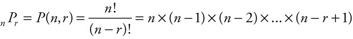
To find the permutation of n elements taken r at a time in Excel, locate your cursor in a spreadsheet cell, activate the Insert Function toolbar button, and select the category: Statistical. In the large window, scroll down the list and select the function: PERMUT. With your cursor active in the field for Number, type n, the total number of elements in the set. With your cursor active in the field for Number chosen, type r, the number of elements to be selected. Click OK. The value of the permutation will appear in the spreadsheet cell. Alternatively, the permutation of n things taken r at a time can be found directly in Excel. Simply type the function: =permut(n, r) in a spreadsheet cell.

2.1.9 Quartile

In addition to finding the median, or 50th percentile, and other percentiles as identified above, we may want to find a particular quartile. Since the second quartile is the median and the fourth quartile is the maximum value in the set of data, the most frequently used quartiles are the first and third quartile. The first quartile is the value below which 25% of the data values fall and above which 75% of the values in the set fall. The third quartile is the value below which 75% of the data values fall and above which 25% of the values in the set fall. One of the simplest procedures to find the first and third quartiles by hand is to simply apply the procedure for finding the location of the median to the lower half of the data set, yielding the first quartile, and to the upper half of the data set, yielding the third quartile.

To find the first quartile in Excel, locate your cursor in a spreadsheet cell, activate the Insert Function toolbar button, and select the category: Statistical. In the large window, scroll down the list and select the function: QUARTILE. With your cursor active in the field for Array, scroll over the data for which you want to determine a percentile on the spreadsheet beneath the window. In the field below Array, labeled Quart, identify the quartile you are interested in, and click OK. In this function, you simply type in 1, 2, or 3 to find the first, second, or third quartile, respectively. You should be aware that, while there is broad consensus on the procedure to use in finding the median or second quartile, some numeric differences may exist in the value Excel identifies as either the first or the third quartile in comparison to other numeric procedures used to find the quartile of interest.

2.1.10 StDev

The standard deviation is an important measure of spread within a set of numeric data. It is used frequently in statistics to determine how common or how unusual a value is in comparison to other values. When the values under consideration represent the entire population of possible data, the standard deviation of that population is denoted by the symbol s, or sigma. When the values in the data set represent a sample taken from a larger population, the standard deviation for the sample is denoted by the symbol s.

To find the sample standard deviation for a set of data, locate your cursor in a spreadsheet cell, activate the Insert Function toolbar button, and select the category: Statistical. In the large window, scroll down the list and select the function: STDEV. With your cursor active in the field for Number 1, scroll over the data for which you want to calculate the standard deviation on the spreadsheet beneath the window and click OK. The value for the standard deviation will appear in the spreadsheet cell. Alternatively, the sample standard deviation for a set of data can be found directly in Excel. Simply type the function: =stdev(range of data) in a spreadsheet cell. As with the other statistical functions, the standard deviation for two or more columns or rows of data can also be found.

The standard deviation for a set of data is denoted by the symbol s and represents a measure of the spread that exists among the data in the sample.

The Question

A sample of eight different vehicles in the corporate car pool is selected and their city mileages per gallon of fuel are measured, producing the values 19.7, 17.6, 21.4, 18.3, 19.5, 18.2, 19.0, and 18.9 mpg. Find the standard deviation among the mileages in the sample.

Answer

s = 1.1683

Using Excel

Enter the data in individual cells A1 through A8. With your cursor in cell A9, activate the Insert Function button, select the Statistical category, highlight STDEV, and click OK. Activate your cursor in the field for Number 1 and then scroll your cursor over cells A1 through A8 containing the data. Click OK. Excel will return the value of the standard deviation, 1.1683, in cell A9. This is equivalent to the procedure outlined in Chapter 1, Example 1.3.

Discussion

The standard deviation among the mileages for the sample of eight cars is s = 1.1683 mpg. The standard deviation can be used to talk about what percent of the data values in the set fall, for example, 2 or 3 units of standard deviation on either side of the mean.

 

2.1.11 StDevP

In the study and use of statistics, it is important to know whether the value is formed using all elements in the population or whether it is based on a random sample of elements taken from the population. When the data set represents the entire population of all values, the standard deviation for the population is s, or sigma. There are different equations used to calculate a sample standard deviation and a population standard deviation, so Excel makes it clear among its statistical functions which standard deviation is formed based on a sample (=STDEV) and which standard deviation is formed over the entire population (=STDEVP).

To find the population standard deviation for a set of data, locate your cursor in a spreadsheet cell, activate the Insert Function toolbar button, and select the category: Statistical. In the large window, scroll down the list and select the function: STDEVP. With your cursor active in the field for Number 1, scroll over the data for which you want to calculate the standard deviation on the spreadsheet beneath the window and click OK. The value for the standard deviation will appear in the spreadsheet cell. Alternatively, the population standard deviation for a set of data can be found directly in Excel. Simply type the function: =stdevp(range of data) in a spreadsheet cell. As with the other statistical functions, the standard deviation for two or more columns or rows of data can also be found.

2.1.12 Var

The variance is also an important measure of spread within a set of numeric data. It is the square of standard deviation and, like standard deviation, is used frequently in statistics to determine how common or how unusual a value is in comparison to other values. When the other values in the data set represent a sample taken from a larger population, the variance for the sample is denoted by the symbol s2.

To find the sample variance for a set of data, locate your cursor in a spreadsheet cell, activate the Insert Function toolbar button, and select the category: Statistical. In the large window, scroll down the list and select the function: VAR. With your cursor active in the field for Number 1, scroll over the data for which you want to calculate the variance on the spreadsheet beneath the window and click OK. The value for the sample variance will appear in the spreadsheet cell. Alternatively, the sample variance for a set of data can be found directly in Excel. Simply type the function: =var(range of data) in a spreadsheet cell. As with the other statistical functions, the variance for two or more columns or rows of data can also be found.

2.1.13 VarP

When the other values in the data set represent all values in a given population, the variance for the population is denoted by the symbol s2.

To find the population variance for a set of data, locate your cursor in a spreadsheet cell, activate the Insert Function toolbar button, and select the category: Statistical. In the large window, scroll down the list and select the function: VARP. With your cursor active in the field for Number 1, scroll over the data for which you want to calculate the variance on the spreadsheet beneath the window and click OK. The value for the population variance will appear in the spreadsheet cell. Alternatively, the population variance for a set of data can be found directly in Excel. Simply type the function: =varp(range of data) in a spreadsheet cell. As with the other statistical functions, the population variance for data contained in two or more columns or rows of data can also be found.

2.2 Inserting Selected Math & Trig Functions

The Math & Trig category under the Insert Function toolbar button has nearly 70 different functions listed. We introduce ten of those most useful to routine statistical and financial calculations.

2.2.1 ABS

The absolute value of an integer is the value of the integer without regard to its sign. So the absolute value of +20 and the absolute value of -20 are both 20. The notation for the absolute value of n is |n|.

To find the absolute value of an integer in Excel, locate your cursor in a spreadsheet cell, activate the Insert Function toolbar button, and select the category: Math & Trig. In the large window, select the function: ABS. With your cursor active in the field for Number, highlight the spreadsheet cell for which you want the absolute value on the spreadsheet beneath the window, and click OK. The absolute value will appear in the spreadsheet cell. Alternatively, the absolute value of a number can be found directly in Excel. Type either =ABS(cell with the value) or =ABS(the value itself) in a spreadsheet cell.

2.2.2 Combin

A combination gives the number of ways a subset of objects can be taken from a larger set regardless of any particular order. A combination of a subset of r objects selected from a set of n objects is smaller than a permutation of the same objects because the order in which the r objects occur is not important in a combination. Since r objects can be arranged in r! different ways, the value of a combination is that of a permutation divided by r!

.

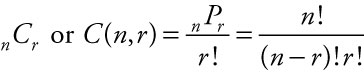Even though a combination is closely related to a permutation, the combination function is located under the Math & Trig category while the permutation function is located under the Statistical category of the Insert Function toolbar button. So, to find the combination of n elements taken r at a time in Excel, locate your cursor in a spreadsheet cell, activate the Insert Function toolbar button, and select the category: Math & Trig. In the large window, scroll down the list and select the function: COMBIN. With your cursor active in the field for Number, type n, the total number of elements in the set. With your cursor active in the field for Number chosen, type r, the number of elements to be selected. Click OK. The value of the combination will appear in the spreadsheet cell. Alternatively, the combination of n things taken r at a time can be found directly in Excel. Simply type the function: =combin(n,r) in a spreadsheet cell.

A combination identifies the number of ways a subset of items with a specific characteristic can be selected from a broader population of objects when the order in which they occur is not important. Being able to evaluate a combination can help us establish how likely a particular event is to occur.

The Question

In how many ways can we select three items to test from a total shipment of 26 items?

Answer

C (26, 3) = 2600

Using Excel

Locate your cursor in a cell on the spreadsheet. Activate the Insert Function button, select the Math & Trig category, highlight COMBIN, and click OK. Activate your cursor in the field for Number and enter the total number of items, 26, from which we can pick. Activate your cursor in the field Number_chosen and enter the number of items you are selecting, 3. Click OK. Excel will return the value of the combination, 2600.

Discussion

There are 2600 unique sets of three items that can be selected from a total number of 26 items. So if we labeled each item with a unique letter A to Z, there would be 2600 different groups of three letters: ABC, ABD, ABE, …. Different orderings of the items are not counted separately, so as long as items A, B, and C are the three items selected to test, that is only counted as one group. So ABC, ACB, BAC, BCA, CAB, and CBA are all considered one group and counted only once in the 2600 unique sets.

 

2.2.3 Int

Using the nearest integer is important in some statistical computations. The integer function in Excel rounds a number down to the integer at or below the number regardless of the size of the decimal component of its value. So, the integer function returns 5 for the number 5.013 as well as for the number 5.987. The integer function returns -2 for the number -1.7 as well as for the number -1.02.

To apply the integer function in Excel, locate your cursor in a spreadsheet cell, activate the Insert Function toolbar button, and select the category: Math & Trig. In the large window, scroll down the list and select the function: INT. With your cursor active in the field for Number, highlight the spreadsheet cell for which you want the integer on the spreadsheet beneath the window, and click OK. The value of the integer will appear in the spreadsheet cell. Alternatively, the integer can be found directly in Excel. Type either =int(cell with the value) or =int(the value itself) in a spreadsheet cell.

2.2.4 Ln

Besides providing a model to describe some logarithmic growth patterns, logarithms play an important role in financial calculations. In exponential notation, a value is a base raised to an exponent, or value = baseexponent. The same relationship can be expressed in logarithmic notation as logbase value = exponent. Stated simply, logarithms are exponents. A frequently used base for logarithms is the number e, which is approximated by 2.71828. A logarithm with a base e is called a natural logarithm, denoted by the symbol ln rather than log. So, loge x = ln x, and represents the exponent to which e is raised to equal the value x.

To find the natural logarithm of a value in Excel, locate your cursor in a spreadsheet cell, activate the Insert Function toolbar button, and select the category: Math & Trig. In the large window, scroll down the list and select the function: LN. With your cursor active in the field for Number, highlight the spreadsheet cell containing the value you want for which the natural logarithm on the spreadsheet beneath the window, and click OK. The value of the natural logarithm will appear in the spreadsheet cell. Alternatively, the natural logarithm can be found directly in Excel. Type either =ln(cell with the value) or =ln(the value itself) in a spreadsheet cell.

2.2.5 Log10

Because our number system is organized on a base of 10, common logarithms are computed on a base of 10. In mathematics, we refer to logarithms in base 10 so frequently that we often do not specify that 10 is the base. So, for example, log10 1000 = 3 is often written simply log 1000 = 3. In Excel, however, we must specify the base of 10 in the function name.

To find the common logarithm of a value in Excel, locate your cursor in a spreadsheet cell, activate the Insert Function toolbar button, and select the category: Math & Trig. In the large window, scroll down the list and select the function: LOG10. With your cursor active in the field for Number, highlight the spreadsheet cell containing the value you want for which the common logarithm on the spreadsheet beneath the window, and click OK. The value of the common logarithm will appear in the spreadsheet cell. Alternatively, the common logarithm can be found directly in Excel. Type either =log10(cell with the value) or =log10(the value itself) in a spreadsheet cell.

Logarithms give us a way to evaluate exponents directly in lieu of relying on trial and error. Logarithms are useful evaluating growth rates in biology and in some areas of finance.

The Question

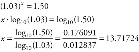
How many years does it require for $1.00 to become $1.50 at a compound interest rate of 3% compounded annually?

Answer

Using Excel

Enter the value 1.50 in cell A10 on a spreadsheet. Enter the value 1.03 in cell A11. Locate your cursor in cell B10. Activate the Insert Function button, select the Math & Trig category, highlight LOG10, and click OK. Activate your cursor in the field for Number and click on cell A10 to evaluate the log base 10 of 1.50. Click OK. Excel will return the log base 10 of 1.50 as 0.176091 in cell B10. Move your cursor over the lower right corner of cell B10 until your cursor turns from a hollow plus to a solid plus sign. Hold your left mouse button down and drag the function into cell B11. Release the left button. Excel will return the value of the log base 10 of 1.03 as 0.012837 in cell B11. To complete the final step, activate your cursor in cell B12 and type: = B10/B11. When you hit enter, Excel will return the final answer, 13.71724, in cell B12.

Discussion

It will require better than 13.7 years for $1.00 to become $1.50 if left in an account that compounds 3% annually.

 

2.2.6 Round

Often what we need is not the exact value of a calculation but a rounded value of the calculation. For example, applying a periodic interest rate to determine an updated account balance requires the calculation be rounded to two digits beyond the decimal point. When an investor submits an amount to purchase shares in a stock or bond fund, the number of shares purchased at the market rate are reported at the thousandths level. The round function in Excel requires two inputs: (1) the number to be rounded and (2) the number of digits beyond the decimal point the function should return. Once the number of digits is specified, Excel evaluates the digit to the right of the number of digits specified and rounds up if that digit is 5 or more and rounds off if that digit is 4 or less.

To apply the rounding function in Excel, locate your cursor in a spreadsheet cell, activate the Insert Function toolbar button, and select the category: Math & Trig. In the large window, scroll down the list and select the function: ROUND. With your cursor active in the field for Number, highlight the spreadsheet cell for which you want the rounded value on the spreadsheet beneath the window. With your cursor active in the field for num_digits, type the number of significant digits you want the number rounded to. Click OK. The rounded value will appear in the spreadsheet cell. Alternatively, the value can be rounded directly in Excel. Type either =round(cell with the value,number of digits) or =round(the value itself,number of digits) in a spreadsheet cell.

2.2.7 SQRT

We often need to take a square root of a value. In statistics, for example, the square root of variance is standard deviation.

To find the square root of a value in Excel, locate your cursor in a spreadsheet cell, activate the Insert Function toolbar button, and select the category: Math & Trig. In the large window, scroll down the list and select the function: SQRT. With your cursor active in the field for Number, highlight the spreadsheet cell containing the value you want for the square root on the spreadsheet beneath the window, and click OK. The value of the square root will appear in the spreadsheet cell. Alternatively, the square root can be found directly in Excel. Type either =sqrt(cell with the value) or =sqrt(the value itself) in a spreadsheet cell.

The square root of a number is the value, when multiplied by itself, equals the given number. So, for instance, the square root of 16 is 4, because 4 ⋅ 4 = 16. The square root is an integer only when the number itself is a perfect square.

The Question

Evaluate the square root of 70.

Answer

Using Excel

Locate your cursor in a cell on the spreadsheet. Activate the Insert Function button, select the Math & Trig category, highlight SQRT, and click OK. Activate your cursor in the field for Number and enter the number 70. Click OK. Excel will return the value of the square root of 70 as 8.3666.

Discussion

The square root of 70 is approximately 8.3666. That is, if you multiply 8.3666 times itself, you get nearly 70. Some error is introduced due to rounding. The value 8 times itself is 64, and the value 9 times itself is 81. So it makes sense that the square root of 70 should fall between 8 and 9, since 70 falls between 64 and 81.

 

2.2.8 Sum

Summing columns or rows of data is important in many applications. From simple activities like reconciling an account balance to complex applications like calculating a monthly payment on a loan, the summation function plays a key role in basic calculations. In statistics, the sum is the basis for calculating both the mean and the variance.

In acknowledging the frequency with which users of Excel need to access the sum for a stream of data, Excel programmers placed a separate AutoSum button on the upper toolbar: Σ . To find the sum of a set of data, locate your cursor in a spreadsheet cell, activate the AutoSum button, then scroll over the data for which you want to calculate the sum on the spreadsheet beneath the window, and click OK. The value for the sum will appear in the spreadsheet cell. Alternatively, you can access the summation function within the Insert Function toolbar button under the Math & Trig category. Scroll down and select the SUM function. With your cursor active in the field for Number 1, scroll over the data for which you want to calculate the sum on the spreadsheet beneath the window and click OK. The value for the sum will appear in the spreadsheet cell. The sum for a set of data can also be found directly in Excel. Simply type the function: =sum(range of data) in a spreadsheet cell. As with the other Excel functions, the sum for data contained in two or more columns or rows of data can also be found.

To find the sum of a set of data, we will return to the data for Example 2.1 that were entered in cells A1 through A8 on the Excel spreadsheet.

The Question

A sample of eight different vehicles in the corporate car pool is selected and their city mileages per gallon of fuel are measured, producing the values 19.7, 17.6, 21.4, 18.3, 19.5, 18.2, 19.0, and 18.9 mpg. Find the sum of the sampled values.

Answer

Using Excel

Enter the data in individual cells A1 through A8. With your cursor in cell A9, activate the Insert Function button, select the Math & Trig category, highlight SUM, and click OK. Activate your cursor in the field for Number1 and scroll your cursor over cells A1 through A8 containing the data. Click OK. Excel will return the sum of the set, 152.6, in cell A9.

Discussion

The total of the eight values added together is 152.6. As noted in Chapter 1, Example 1.1, the sum of a set of numbers can be the first step in finding the average for the numbers.

 

2.2.9 Trunc

Occasionally what we need is neither a rounded nor the nearest integral value of a calculation but the last value of the calculation specified to a certain number of decimal places. The truncating function in Excel levels a number back to the last value given a certain number of decimal places. So, the truncating function for two decimal values returns 5 for the number 5.013 as well as for the number 5.987. The truncating function for two decimal values returns -2 for the number -1.99 and -3 for the number -2.05. The truncating function for one decimal value returns -1.9 for the number -1.99 but -1.4 for the number -1.46. The truncating function in Excel requires two inputs: (1) the number to be rounded and (2) the number of digits beyond the decimal point the function should evaluate.

To apply the truncating function in Excel, locate your cursor in a spreadsheet cell, activate the Insert Function toolbar button, and select the category: Math & Trig. In the large window, scroll down the list and select the function: TRUNC. With your cursor active in the field for Number, highlight the spreadsheet cell for which you want the rounded value on the spreadsheet beneath the window. With your cursor active in the field for num_digits, type the number of significant digits you want to be considered. Click OK. The truncated value will appear in the spreadsheet cell. Alternatively, the value can be rounded directly in Excel. Type either =trunc(cell with the value,number of digits) or =trunc(the value itself,number of digits) in a spreadsheet cell.

2.3 Inserting Selected Financial Functions

The Financial category under the Insert Function toolbar button has nearly 90 different functions listed. Many of the automated functions are designed to conduct calculations for complex financial applications. We introduce a few of the more frequently used financial functions.

2.3.1 Effect

When interest is assessed on the balance of an account on any other than an annual basis, the annual interest rate on the account does not allow for the compounding effect taking place. The effective interest rate, r_E, is the simple interest rate that, when applied to the balance of the account, would generate the same amount of interest as generated by the annual interest rate compounded over the year. Because of compounding, the effective interest rate is higher than the stated annual rate. Credit card accounts usually announce both the annual and the effective rates of interest.

To find the effective interest rate in Excel, locate your cursor in a spreadsheet cell, activate the Insert Function toolbar button, and select the category: Financial. In the large window, scroll down the list and select the function: EFFECT. With your cursor active in the field for Nominal_rate, enter the stated annual interest rate as a decimal equivalent. With your cursor active in the field for Npery, enter the number of compounding periods per year and click OK. The value of the effective interest rate will appear in the spreadsheet cell. Alternatively, the effective interest rate can be found directly in Excel. Type =effect(stated annual interest rate,number of compounding periods per year) in a spreadsheet cell.

To find the simple interest rate that, when applied to the balance of an account, would generate the same amount of interest as generated by the annual interest rate compounded over the year, we will use the effective interest rate function in Excel.

The Question

A store account identifies 18% interest rate compounded monthly. Find the effective interest rate that is equivalent to this compounded annual rate.

Answer

r_E = 0.195618 or approximately 19.56%

Using Excel

Locate your cursor in a cell on the spreadsheet. Activate the Insert Function button, select the Financial category, highlight EFFECT, and click OK. Activate your cursor in the field for Nominal rate and enter the number 0.18, the stated annual simple interest rate. Activate your cursor in the field for Npery and enter the number 12, the number of interest or payment periods in a year. Click OK. Excel will return the value of the effective rate of return, 0.195618, in the cell.

Discussion

If you divide the annual interest rate 0.18 by 12, the monthly interest rate is 0.015. When you raise (1 + 0.015) to the power of 12, you will get: (1 + 0.015)2 = 0.195618, which is the effective interest rate for that account.

 

2.3.2 FV

The future value of a stream of constant payments made each interest period is called the future value of an annuity. It represents the value of the account at the end of the final deposit and is comprised of the sum of the periodic payments plus all compound interest accrued over the life of the account.

To find the future value of a stream of payments in Excel, locate your cursor in a spreadsheet cell, activate the Insert Function toolbar button, and select the category: Financial. In the large window, scroll down the list and select the function: FV. With your cursor active in the field for Rate, enter the periodic interest rate as a decimal equivalent. If, for example, the interest rate is 6% compounded monthly, the periodic interest rate would be 0.06 ÷ 12 = 0.005. With your cursor active in the field for Nper, enter the total number of compounding periods over the life of the account. For example, you would enter 36 for an account of 3 years duration with monthly compounding, since 3 × 12 = 36. With your cursor active in the field for PMT, enter as a negative value the constant amount deposited with each payment. Not required are entries in the fields for Pv or Type. Click OK. The future value of the stream of payments will appear in the spreadsheet cell. Alternatively, the future value can be found directly in Excel. Type =fv(periodic interest rate,number of interest periods over the life of the account,value of the constant payment made to the account as a negative value) in a spreadsheet cell.

To find the future value of an ordinary annuity, we will use Excel’s built-in function, FV.

The Question

Tran is going on active duty for a 24-month assignment overseas. He anticipates he will be able to save $8.99 a month by not streaming first-run movies while he is on active duty. Instead of incurring the standard charge to his credit card during the 24-month period, Tran elects to authorize his bank to withdraw the amount from his checking account as an automatic payment into a savings account that earns 3% annual interest rate compounded monthly. How much will be in the account at the end of the 24-month duty period when he returns home?

Answer

FV = $222.08

Using Excel

Locate your cursor in a cell on the spreadsheet. Activate the Insert Function button, select the Financial category, highlight FV, and click OK. Activate your cursor in the field for Rate and enter the number 0.03/12, the annual interest rate converted to a periodic interest rate. Activate your cursor in the field for Nper and enter the number 24, the number of interest or payment periods over which the payment will be made. Activate your cursor in the field for Pmt and enter the value -8.99, the amount of the monthly payment. Click OK. Excel will return the future value of the account, $222.08, in the cell.

Discussion

The future value of the stream of 24 payments each for $8.99 into Tran’s account earning 3% interest will be worth $222.08 at the end of 24 months. The payments themselves account for $8.99 × 24 = $215.76, and there was a total of $6.32 earned in interest over the 24-month period.

 

2.3.3 NPV

The net present value (NPV) function produces the present value of a stream of irregular payments assuming a given discount rate. The argument for the function is in the form of =NPV(discount rate, range of future payments).

2.3.4 PMT

The periodic payment needed to pay off the present value of a loan over a specific number of payments and interest rate is a useful calculation for consumers. It includes payment to the principal and interest due on the outstanding balance, and is calculated so that the constant payment over the specified number of payments fully covers the outstanding balance and its interest.

To find the periodic payment in Excel, locate your cursor in a spreadsheet cell, activate the Insert Function toolbar button, and select the category: Financial. In the large window, scroll down the list and select the function: PMT. With your cursor active in the field for Rate, enter the periodic interest rate as a decimal equivalent. If, for example, the interest rate is 6% compounded monthly, the periodic interest rate would be 0.06 ÷ 12 = 0.005. Alternatively, you can enter the annual interest rate, the division sign “/” followed by 12. With your cursor active in the field for Nper, enter the total number of compounding periods over the life of the account. For example, you would enter 36 for an account of 3 years duration with monthly compounding, since 3 × 12 = 36. With your cursor active in the field for PV, enter the total amount due. Usually that is the outstanding balance of the asset being purchased with payments made over time. Click OK. The value of the payment will appear in the spreadsheet cell. Alternatively, the effective interest rate can be found directly in Excel. Type =pmt(periodic interest rate,total number of periods over the life of the loan,outstanding balance of the asset) in a spreadsheet cell.

We will use the programmed function PMT to find the amount of a payment required each period to pay off in a stated number of payments the present value owed, given an assumed interest rate.

The Question

Mario and Luz buy a living room furniture set which, with tax and delivery, totals $3895.92. They put $300 down and plan to pay the remaining balance over 36 monthly payments, with 2½% annual interest rate. How much each month will they need to plan to pay it off in the stated amount of time?

Answer

PMT = $103.78

Using Excel

Locate your cursor in a cell on the spreadsheet. Activate the Insert Function button, select the Financial category, highlight PMT, and click OK. Activate your cursor in the field for Rate and enter the number 0.002083 or 0.025/12, the annual interest rate converted to a periodic interest rate. Activate your cursor in the field for Nper and enter the number 36, the number of interest or payment periods over which the payment will be made. Activate your cursor in the field for PV and enter the value 3595.92, the amount they currently owe when they take possession of the furniture set, the amount of the monthly payment. Click OK. Excel will return the value of the monthly payment required to pay the debt off in 36 monthly payments with 2½% annual interest rate, $103.78, in the cell.

Discussion

The total value of the stream of payments will equal $103.78 × 36 = $3,736.08. By making payments, Mario and Luz will have paid $140.16 in total interest above the outstanding amount of $3,595.92 due when they took possession of the asset.

 

2.3.5 PV

The present value of a stream of constant, equally-timed payments made into the future at a set interest rate each interest period is called the present value of an annuity. It represents the lump sum that would need to be deposited today to equal a stream of constant payments into the future earning the same interest rate.

To find the present value of a stream of payments in Excel, locate your cursor in a spreadsheet cell, activate the Insert Function toolbar button, and select the category: Financial. In the large window, scroll down the list and select the function: PV. With your cursor active in the field for Rate, enter the periodic interest rate as a decimal equivalent. If, for example, the interest rate is 6% compounded monthly, the periodic interest rate would be 0.06 ÷ 12 = 0.005. With your cursor active in the field for Nper, enter the total number of compounding periods over the life of the account. For example, you would enter 36 for an account of 3 years duration with monthly compounding, since 3 × 12 = 36. With your cursor active in the field for Pmt, enter as a negative value the constant amount deposited with each payment. Not required are entries in the fields for Fv or Type. Click OK. The present value of the stream of payments will appear in the spreadsheet cell. Alternatively, the present value can be found directly in Excel. Type: =pv(periodic interest rate,number of interest periods over the life of the account,value of the constant payment made to the account as a negative value) in a spreadsheet cell.

To find the present value of an ordinary annuity, we will use Excel’s built-in function, PV.

The Question

Sharnell won a state-sponsored lottery that guarantees her $2,500 per month for 25 years. Assuming a constant annual interest rate of 2% over the 25 years, how much in a lump sum would have to be deposited into an account today earning 2% annual interest compounded monthly to equal this stream of payments?

Answer

PV = $589,825.27

Using Excel

Locate your cursor in a cell on the spreadsheet. Activate the Insert Function button, select the Financial category, highlight PV, and click OK. Activate your cursor in the field for Rate and enter the number 0.02/12, the annual interest rate converted to a periodic interest rate. Activate your cursor in the field for Nper and enter the number 300, the number of interest or payment periods over which the payment will be made. Alternatively, you can enter 12*25 in the Nper field, since there will be 12 payments a year made over 25 years. Activate your cursor in the field for Pmt and enter the value -2500, the amount of the monthly payment. Click OK. Excel will return the present value of the stream of future payments, $589,825.27, in the cell.

Discussion

The present value of the stream of 300 monthly payments each for $2,500 to Sharnell assuming 2% interest is $589,825.27. The payments themselves would have totaled $2500 × 300 = $750,000 over time, which is being discounted $160,174.73 to today in recognition of the interest that will be generated over the years that the account funds the stream of payments.

 

2.3.6 RATE

The periodic interest rate for a loan can be computed based on the periodic payment, the number of payment periods in the life of the loan, and the present value of the asset being purchased with payments made over time.

To find the periodic interest rate in Excel, locate your cursor in a spreadsheet cell, activate the Insert Function toolbar button, and select the category: Financial. In the large window, scroll down the list and select the function: RATE. With your cursor active in the field for Nper, enter the total number of compounding periods over the life of the account. For example, you would enter 36 for an account of 3 years duration with monthly compounding, since 3 × 12 = 36. With your cursor active in the field for Pmt, enter as a negative value the constant amount deposited with each payment. With your cursor active in the field for Pv, enter the outstanding balance owed on the asset being purchased with payments made over time. Not required are entries in the fields for Fv or Type. Click OK. The periodic interest rate will appear in the spreadsheet cell. Alternatively, the present value can be found directly in Excel. Type: =rate(periodic interest rate,value of the constant payment made to the account as a negative value,present value of the asset being purchased with payments made over time) in a spreadsheet cell.