Abercrombie & Fitch Co.—Regression Case Study1
Introduction
The Family Clothing Store industry, in which Abercrombie & Fitch Co. (A&F) operates, is highly fragmented and is dominated by a large number of small retailers, each with a low market share of the total industry. The top four players in this industry are A&F, Gap Inc., American Eagle Outfitters, Inc., and Ross Stores. These four companies collectively account for about 40% of the market. A&F generally charges higher prices compared with similar merchandise at Gap and American Eagle. The company was founded in 1892 and is headquartered in New Albany, Ohio.
The Company’s stores offer knit and woven shirts, graphic t-shirts, fleece, jeans and woven pants, shorts, sweaters, and outerwear. A&F operates over one thousand stores in the United States, Canada, and the United Kingdom. It also sells its products through the Internet and catalogues.
The A&F brand targets college students, the RUEHL Brand, launched in 2005 and dropped in 2008, was a mix of business casual and trendy fashion, created to appeal to the modern-minded and post-college customers. In early 2007, the company launched another brand, Gilly Hicks, which specializes in women’s underwear, sleepwear, personal care products, and at-home products.
The Data
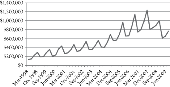
To build a regression model for sales of A&F the dependent variable is sales of A&F on a quarterly basis and in thousands of dollars.2 These values are shown in Figure 10.1 as a time-series plot constructed in Excel. As you see, sales increased from the beginning of this series until the economic downturn in 2008. You also see sharp peaks that may represent seasonality in their sales. For A&F, the fiscal year runs from February to January, which makes February, March, and April the first quarter and subsequently November, December, and January the last quarter. The data are labeled using the middle month of the quarter. Thus, March represents the first quarter and December represents the fourth quarter of each year.
When you think about constructing a model for a company’s sales one of the first things that comes to mind is some measure of consumer buying power. You may know the concept of a “normal good.” The products sold by A&F would be considered normal goods. A normal good is one for which sales would increase as income increases. For this example, personal income (PI) in billions of dollars is used as a measure of buying power.
Unemployment often affects retail sales beyond the effect that unemployment has on income. If consumers are unemployed, or if they are employed but have concerns about losing their jobs, their purchasing behavior is likely to change. In the case of A&F the clothing and other items they sell would be considered discretionary goods. Thus, in times of high unemployment, consumers may put off purchases from a store such as A&F.
Most retail sales have considerable seasonality. You can see this in Figure 10.1. Therefore, you would want to use dummy variables to evaluate the degree and nature of seasonality.
During the period considered A&F started a new brand called “RUEHL” and another called “Gilly Hicks.” For each brand you could create a dummy variable with a one when that brand existed and zero otherwise. The RUEHL brand was only on the market from 2005 through 2007; so the dummy variable for RUEHL is a one in the 12 quarters covering 2005 through 2007. The other brand, Gilly Hicks, was started in early 2007. The dummy variable for Gilly Hicks is therefore a one starting in the first quarter of 2007 through the end of the data, and zero prior to 2007.
The Hypotheses
When you do a regression analysis you should think carefully about the expectations you have for each independent variable. Do you expect a positive or negative coefficient for each of the independent variables? For the A&F regression model you have the following potential independent variables: personal income (PI), the unemployment rate (UR), seasonal dummy variables (Q1, Q2, Q3, and Q4), RUEHL brand, and Gilly Hicks brand. Thus, you should think about the direction of the impact each of these could have on A&F sales.
Hypothesis 1. The Expected Influence of Income
When the personal income of individuals increase, they tend to purchase more as their buying power increases. On the other hand, when the personal income falls, their purchasing power is reduced and they lower their purchases of normal goods. Thus, your research hypothesis is that the true regression slope (β) between sales and income should be positive. Thus, your hypotheses for personal income are:
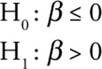
This form of the statistical test is appropriate for personal income, because you expect a direct relationship between sales of A&F and personal income. You expect an increase (decrease) in personal income to cause an increase (decrease) in A&F sales.
Hypothesis 2. The Expected Influence of the Unemployment Rate
You might expect that there is more than an income effect of unemployment on the sale of consumer goods. You would expect that the sales of A&F would have an inverse relationship with the unemployment rate. Thus, your hypotheses for the unemployment rate are:
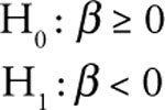
If the unemployment rate increases, then the A&F sales would be expected to decreases and vice versa.
Hypothesis 3. Seasonal Dummy Variables
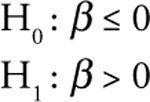
You might expect that A&F would experience the greatest sales activity during the fall season due to the back-to-school sales as well as in the last part of the year due to holiday gift buying. The first quarter of the year is typically the lowest quarter for retail sales of almost all types of products. Thus, it makes sense to use the first quarter as the base period. As a result, you would expect sales to be higher in quarters two, three, and four than in the first quarter of each year. Thus, your hypotheses for Q2, Q3, and Q4 are all the same as follows:
Hypothesis 4. RUEHL and Gilly Hicks
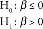
With regard to the dummy variables for the RUEHL and the Gilly Hicks brands, you would expect a positive relationship to overall sales. Remember that these two dummy variables are equal to 1 when the brand exists and equal to 0 when the brand does not exist. Thus the hypotheses for each of these brands (RUEHL and Gilly Hicks) would be:
The Regression Models
To help you see the development of regression models, four models of A&F sales are discussed in this section. The first includes only one independent variable (personal income), the second adds unemployment, the third also includes seasonal dummy variables, and finally, the fourth model adds the two dummy variables related to the RUEHL and Gilly Hicks brands.
For each model you will see the Excel regression results and a graph of the actual A&F sales compared with the predictions from each model. You will also see a brief discussion of the five-step evaluation of each model.
Model 1. Sales as a Function of Personal Income
First, look at the regression results from Excel in Table 10.1. As you see, the Excel regression output has been edited to help you concentrate on the most important parts of the tables. These results will form the basis for your five-step evaluation of the first model.
Table 10.1. A&F Sales as a Function of Personal Income
|
S = f(PI) |
||||
|
Regression statistics |
||||
|
Multiple R |
0.882 |
|
DW = 1.552 |
|
|
R-square |
0.778 |
|||
|
Adjusted R-square |
0.773 |
|||
|
Standard error |
131,967 |
|||
|
Observations |
47 |
|
|
|
|
ANOVA |
||||
|
|
df |
F |
Sig F |
|
|
Regression |
1 |
157.668 |
0.000 |
|
|
Residual |
45 |
|||
|
Total |
46 |
|||
|
|
Coefficients |
t Stat |
p-Value |
P/2 |
|
Intercept |
–903,489 |
–7.773 |
0.000 |
0.000 |
|
PI |
165.573 |
12.557 |
0.000 |
0.000 |
The most important statistical results are in bold in the Excel output in Table 10.1. From the Coefficients column you can write the equation for this model as:
![]()
Step 1: Is the Model Logical?
You would expect that as consumers’ incomes increase A&F would sell more goods. Therefore, the positive (+) sign for the coefficient (slope) related to income is logical.
Step 2: Is the Slope Term Significantly Positive?
In order to check for statistical significance of the independent variable (PI) the hypothesis for the slope of income is subjected to a one-tailed t-test. If the absolute value of calculated tc is greater than the t-table value at the 95% confidence level (5% significance level), you can reject the null hypothesis. This means that you have empirical support for the research hypothesis. To determine the t-table value, the degree of freedom (df) is calculated as df = n – (k + 1). In this case, n = number of observations in the model = 47 and k = number of independent variables = 1. Thus, df = 47 – (1 + 1) = 45. The t-table value is approximately 1.648 (see Appendix 4B).
The calculated t-ratio for disposable personal income is 12.557. This would be very far into the right tail of the distribution as indicated by a p-value of 0 to three decimal places. In the Excel output table, you see a column that is added for the p-value divided by two (p/2) because you would be doing a one-tailed test and the p-value provided by Excel is for both tails of the distribution. Of course, p/2 is also less than the desired level of significance of 0.05. Thus, there is very little risk of error in rejecting the null hypothesis.
Step 3: What is the Explanatory Power of the Model?
For this bivariate regression model, the explanatory power is measured by the coefficient of determination, R2. The coefficient of determination tells you the percentage of the variation in the dependent variable (A&F sales) that is explained by the one independent variable, personal income (PI). In this model, the coefficient of determination (R2) is 0.778, which means 77.8% of the variation in the A&F sales is explained by this model.
Step 4: Check for Serial Correlation
Because time-series data are used in this model you need to be concerned about possible serial correlation. You can evaluate this using the DW statistic. The DW statistic will always be in the range of 0–4 and as a rule of thumb, a value between 1.5 and 2.5 is suggestive that there may be no serial correlation.
The DW statistic for this model is 1.552. Based on the table in Appendix 4C and the discussion in Appendix 4D you see that du < 1.552 < 2, so Test 4 is satisfied and you can say that no serial correlation exists. For this case, you would use du = 1.544 with n = 40 and k = 1.3
Step 5: Check for Multicollinearity
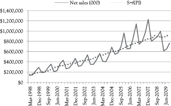
For a simple model with only one independent variable there is no possible multicollinearity. In Figure 10.2, the graph shows the actual A&F sales (solid line) along with the predictions based on Model 1 (dotted line). What do you think is most clearly missing in the model?
Model 2. Sales as a Function of Personal Income and Unemployment Rate
You can now expand Model 1 to include more variables in Models 2–4. Your evaluation of each model should follow the same format as for Model 1. Looking at three more models of sales for A&F will help you understand how models are developed and evaluated.
Suppose that next you decide to add the unemployment rate as an additional independent variable. Again you should first look at the regression results from Excel shown in Table 10.2. Here PI = personal income and UR = unemployment rate.
Table 10.2. A&F sales as a function of Personal Income and the Unemployment Rate
|
S = f(PI,UR) |
||||
|
Regression statistics |
||||
|
Multiple R |
0.916 |
|
DW = 2.126 |
|
|
R-square |
0.839 |
|||
|
Adjusted R-square |
0.832 |
|||
|
Standard error |
113,643 |
|||
|
Observations |
47 |
|
|
|
|
ANOVA |
||||
|
|
df |
F |
Sig F |
|
|
Regression |
2 |
114.649 |
0.000 |
|
|
Residual |
44 |
|||
|
Total |
46 |
|||
|
|
Coefficients |
t Stat |
p-Value |
P/2 |
|
Intercept |
–808,157 |
–7.863 |
0.000 |
0.000 |
|
PI |
193.743 |
14.583 |
0.000 |
0.000 |
|
UR |
–64,867.629 |
–4.084 |
0.000 |
0.000 |
Table 10.3. A&F Sales as a Function of Personal Income, the Unemployment Rate, and Seasonal Dummy Variables for Q3 and Q4
|
S = f(PI,UR,Q3,Q4) |
||||
|
Regression statistics |
||||
|
Multiple R |
0.980 |
|
DW = 1.540 |
|
|
R-square |
0.961 |
|||
|
Adjusted R-square |
0.957 |
|||
|
Standard error |
57,587 |
|||
|
Observations |
47 |
|
|
|
|
ANOVA |
||||
|
|
df |
F |
Sig F |
|
|
Regression |
4 |
255.576 |
0.000 |
|
|
Residual |
42 |
|||
|
Total |
46 |
|||
|
|
Coefficients |
t Stat |
p-Value |
P/2 |
|
Intercept |
–887,092 |
–16.880 |
0.000 |
0.000 |
|
PI |
191.011 |
28.354 |
0.000 |
0.000 |
|
UR |
–60,899.517 |
–7.543 |
0.000 |
0.000 |
|
Q3(Aug–Oct) |
103,851.594 |
5.091 |
0.000 |
0.000 |
|
Q4(Nov–Jan) |
236,556.285 |
11.266 |
0.000 |
0.000 |
The Excel results in Table 10.2 provide the basis for your five-step evaluation of the second model. The most important statistical results are in bold. From the Coefficients column you can write the equation for this model as:
![]()
Step 1: Is the Model Logical?
Again, you expect that as consumers’ incomes increase A&F would sell more goods so the positive (+) sign for the slope related to income is logical. And, you would expect that a higher unemployment would result in lower sales. Thus, the negative slope for UR is logical.
Step 2: Are the Slope Terms Significantly Positive?
Now you need to evaluate each of the two slope terms. Since you now have two independent variables df = n – (k + 1) = 47 – (2 + 1) = 44. Because the closest value for df in your table is 40, you would again use a t-table value of 1.648. For both variables, the calculated t-statistics are well into the tails of the distribution (the upper tail for PI and the lower tail for UR). Further, in both cases p/2 is less than the level of significance of 0.05. This means that you have empirical support for both of the research hypotheses (at greater than a 95% confidence level).
Step 3: What is the Explanatory Power of the Model?
For this multiple regression model, the explanatory power is measured by the coefficient of determination, but now you must use the adjusted R-square. This coefficient of determination tells you the percentage of the variation in the dependent variable (A&F sales) that is explained by PI and the UR. In this model, the coefficient of determination (adjusted R2) is 0.832, which means 83.2% of the variation in the A&F sales is explained by this model. This is an improvement over the bivariate model.
Step 4: Check for Serial Correlation
Again you need to be concerned about possible serial correlation. The DW statistic for this model is 2.126. Based on the table in Appendix 4C and the discussion in Appendix 4D you see that 2 < 2.126 < (4 – du), so Test 3 is satisfied and you can say that no serial correlation exists. For this case, you would use du = 1.600 with n = 40 (rather than n = 47) and k = 2.
Step 5: Check for Multicollinearity
With more than one independent variable you need to look at the correlation matrix for all pairs of independent variables. The correlation between PI and UR is 0.519, so the two variables are not strongly enough correlated to cause a problem. Also, there is no indication in the model of a multicollinearity problem, since both signs for coefficients are as you expect.
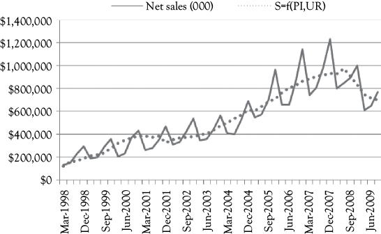
In Figure 10.3, you see a graph that shows the actual A&F sales (solid line) along with the predictions based on Model 2 (dotted line). This model fits a bit better than Model 1 but it is not as good as you would hope. What do you think is still missing?
Model 3. Sales as a Function of PI, UR, and Two Seasonal Dummy Variables (Q3 and Q4)
Having recognized that both Models 1 and 2 failed to account for the seasonal variation in A&F sales, you would naturally try to add seasonal dummy variables. Analysis of the data shows that there is only significant seasonality during the back to school and holiday seasons (quarters Q3 and Q4). Therefore, you only need seasonal dummy variables for these two quarters of each year.
You rely upon the regression results from Excel as shown in Table 10.3 to evaluate Model 3. Here PI = personal income, and UR = the unemployment rate, while Q3 and Q4 represent the corresponding quarters. From the Coefficients column, you can write the equation for this model as:

Step 1: Is the Model Logical?
Again, you expect that as consumers’ incomes increase A&F would sell more goods and as unemployment increases they would be expected to sell less. Thus, a positive sign for the slope related to income is logical as is the negative sign for unemployment. You would expect quarters Q3 and Q4 to have higher sales than the rest of the year due to back to school and holiday shopping. Q3 is a dummy variable equal to 1 every third quarter and 0 otherwise. Q4 is a dummy variable equal to 1 every fourth quarter and 0 otherwise. Thus, the positive coefficients for Q3 and Q4 make sense.
Step 2: Are the Slope Terms Significantly Positive?
Now you need to evaluate all four slope terms. Since you now have four independent variables, df = n – (k + 1) = 47 – (4 + 1) = 42. Again you would use a t-table value of 1.648. For all four variables, the calculated t-statistics are well into the tails of the distribution (the upper tail for PI, Q3, Q4, and the lower tail for UR). Further, in all cases p/2 is less than the desired level of significance of 0.05. This means that you have empirical support for all four of the research hypotheses (at greater than a 95% confidence level).
Step 3: What is the Explanatory Power of the Model?
For this multiple regression model, the explanatory power is again measured by the adjusted R-square. This value tells you the percentage of the variation in the dependent variable (A&F sales) that is explained by PI, UR, and seasonality as measured by Q3 and Q4. In this model, the adjusted R-square is 0.957, which means 95.7% of the variation in the A&F sales is explained by this model. This is a big improvement and helps you to see the importance of using dummy variables for seasonality.
Step 4: Check for Serial Correlation
Again you need to be concerned about possible serial correlation. The DW statistic for this model is 1.540. Based on the table in Appendix 4C and the discussion in Appendix 4D, you see that dl = 1.285 < 1.540 < 1.721 = du so Test 5 is satisfied, which means the test for serial correlation is indeterminate.4 You are not sure that you have or do not have positive serial correlation. One solution may be that you are missing some useful causal (independent) variables.
Step 5: Check for Multicollinearity
With more than one independent variable, you need to look at the correlation matrix for all pairs of independent variables. The correlation matrix is shown in Table 10.4. The correlations between the individual pairs of independent variables in this model are not very high as shown in the correlation matrix in Table 10.4. Also, there is no indication in the model of a multicollinearity problem, since the signs for all four coefficients are as you expect.
Table 10.4. Correlation Matrix for Personal Income (PI), the Unemployment Rate (UR), and Seasonal Dummy Variables for Q3 and Q4
|
PI |
UR |
Q3(Aug–Oct) |
Q4(Nov–Jan) |
|
|
PI |
1.000 |
|||
|
UR |
0.519 |
1.000 |
||
|
Q3 (Aug–Oct) |
0.043 |
0.074 |
1.000 |
|
|
Q4 (Nov–Jan) |
–0.005 |
–0.061 |
–0.324 |
1.000 |
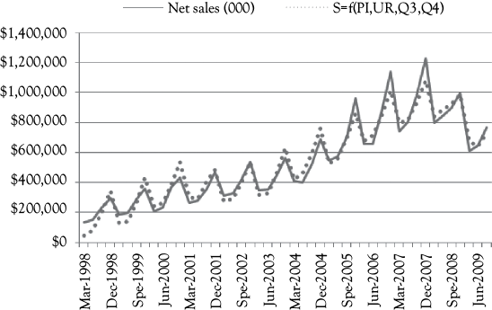
In Figure 10.4, you see a graph that shows the actual A&F sales (solid line) along with the predictions based on Model 3 (dotted line). This model fits much better than Model 2 but may have a positive serial correlation issue.
Model 4. Sales as a Function of Personal Income, Unemployment Rate, Two Seasonal Dummy Variables (Q3 and Q4), and Dummy Variables for Two Brands
During the period for which you have data, A&F added in 2005 then dropped in 2008 the RUEHL brand, and they added the Gilly Hicks brand in 2007. For each quarter in the data, the RUEHL and the Gilly Hicks brands either were or were not part of A&F. Thus, you can create a dummy variable for each brand that equals 1 when the brand was active and 0 otherwise. Now look at the new regression results in which you include PI, UR, Q3, Q4, the RUEHL brand, and the Gilly Hicks brand as independent variables.
These results, as shown in Table 10.5, form the basis for your Five-step evaluation of the fourth (and last) model. From the Coefficients column you can write this equation as:
Table 10.5. A&F sales as a function of Personal Income, the Unemployment Rate, Seasonal dummy variables for Q3 and Q4, and Dummy Variables for the RUEHL and Gilly Hicks brands
|
S = f(PI,UR,Q3,Q4,R,GH) |
||||
|
Regression statistics |
||||
|
Multiple R |
0.985 |
|
DW = 1.868 |
|
|
R-square |
0.971 |
|||
|
Adjusted R-square |
0.966 |
|||
|
Standard error |
50,822 |
|||
|
Observations |
47 |
|
|
|
|
ANOVA |
||||
|
|
df |
F |
Sig F |
|
|
Regression |
6 |
221.087 |
0.000 |
|
|
Residual |
40 |
|||
|
Total |
46 |
|||
|
|
Coefficients |
t Stat |
p-Value |
P/2 |
|
Intercept |
–740,334 |
–9.901 |
0.000 |
0.000 |
|
PI |
156.457 |
12.915 |
0.000 |
0.000 |
|
UR |
–39,031.235 |
–4.199 |
0.000 |
0.000 |
|
Q3(Aug–Oct) |
105,510.792 |
5.851 |
0.000 |
0.000 |
|
Q4(Nov–Jan) |
241,508.876 |
12.934 |
0.000 |
0.000 |
|
RUEHL Brand |
100,586.139 |
3.726 |
0.001 |
0.000 |
|
Gilly Hicks Brand |
49,795.596 |
1.687 |
0.099 |
0.0497 |

In the above regression equation all of the coefficients have all been rounded to a whole number to save space.
Step 1: Is the model logical?
Again, you expect that A&F would sell more goods as PI increases, when it is a third or fourth quarter and when they have the RUEHL and Gilly Hicks brands. You would expect them to have lower sales if unemployment increases. Therefore, all six slope terms in the model have signs for their coefficients that make sense.
Step 2: Are the Slope Terms Significantly Positive?
Now you need to evaluate all six slope terms. Now that you have six independent variables, df = n – (k + 1) = 47 – (6 + 1) = 40. Again you would use a t-table value of 1.648. For the first five variables the calculated t-statistics are well into the tails of the distribution (the upper tail for PI, Q3, Q4, R, and the lower tail for UR). For Gilly Hicks, the calculated t-ratio of 1.687 is only slightly larger than the t-table value of 1.648. How much larger is not important. As long as it is larger than the critical t-table value your 95% confidence level criterion is satisfied. You see that, for all six variables p/2 is less than 0.05, which is your desired significance level (corresponding to a 95% confidence level). This means that you have empirical support for all six of the research hypotheses.
Step 3: What is the Explanatory Power of the Model?
For this multiple regression model, the explanatory power is again measured by the adjusted R2. In this model the adjusted R2 is 0.966, which means 96.6% of the variation in the A&F sales is explained by PI, UR, seasonality, and the existence of the RUEHL and Gilly Hicks brands. This is a slight improvement over Model 3. Of course, as you get close to 100% additional explanatory power becomes increasingly difficult to obtain.
Step 4: Check for Serial Correlation
Again you need to be concerned about possible serial correlation. The DW statistic for this model is 1.868. Based on the table in Appendix 4C and the discussion in Appendix 4D you see that dl = 1.175 < 1.868 < 2.000 so Test 4 is satisfied (n = 40 and k = 6). This means that this model does not have a serial correlation problem.5 By adding two additional variables that have a significant effect on A&F sales has alleviated the potential serial correlation that you observed in Model 3.
Step 5: Check for Multicollinearity
You know that with more than one independent variable you need to look at the correlation matrix for all pairs of independent variables. The correlations between the individual pairs of independent variables in this model are not very high as shown by the correlation matrix below in Table 10.6. Also, there is no indication in the model of a multicollinearity problem, since the signs for all four coefficients are as you expect.
Table 10.6. Correlation Matrix for Personal Income (PI), the Unemployment Rate(UR), Seasonal Dummy Variables for Q3 and Q4, and Dummy Variables for RUEHL and Gilly Hicks
|
PI |
UR |
Q3(Aug–Oct) |
Q4(Nov–Jan) |
RUEHL brand |
Gilly Hicks brand |
|
|
PI |
1.000 |
|
|
|
|
|
|
UR |
0.519 |
1.000 |
|
|
|
|
|
Q3(Aug–Oct) |
0.043 |
0.074 |
1.000 |
|
|
|
|
Q4(Nov–Jan) |
–0.005 |
–0.061 |
–0.324 |
1.000 |
|
|
|
RUEHL brand |
0.470 |
–0.229 |
–0.007 |
0.022 |
1.000 |
|
|
Gilly Hicks brand |
0.755 |
0.456 |
0.022 |
–0.068 |
0.137 |
1.000 |
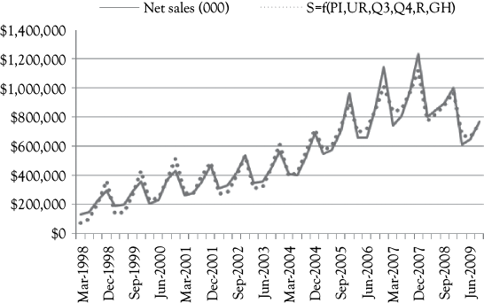
In Figure 10.5, you see a graph that shows the actual A&F sales (solid line) along with the predictions based on Model 4 (dotted line). This model fits very well and does not have a positive serial correlation problem.
Observations
By reading the process of developing and evaluating these models for A&F sales you will have solidified your understanding of multiple regression analysis. You will really learn about regression best by doing regression. You can start by entering the data for annual women’s clothing sales (WCS) data from Table 3.1 as your dependent variable and the year (time index) as your dependent variable. Then do the regression and verify that you get the same results as you saw in chapter 3. After that, start to experiment with your own data.
NOTES
1 We thank Laxmi Subhasini Rupesh for background research related to this case.
2 SEC filings at www.sec.gov.
3 You would use 40 rather than n = 47 because the table only goes as high as 40.
4 For this case, you would use dl = 1.285 and du = 1.721 with n = 40 (rather than n = 47)and k = 4.
5 For this case, you would use dl = 1.175. The 2.000 comes from the rule for Test 4 (see Appendix 4A).

