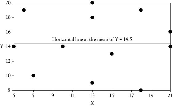
Figure 4.1. Scattergram when X is not a function of Y. The solid line represents the mean value of Y. When no relationship exists, the best estimate of Y for any observed value of X is the mean value of Y (represented by the solid line).
Evaluation of Ordinary Least Squares (OLS) Regression Models
Chapter 4 Preview
When you have completed reading this chapter you will be able to:
• Identify the four steps involved in evaluating a simple regression model.
• Evaluate whether a simple regression model makes logical sense.
• Check for statistical significance of a slope term.
• Identify when it is appropriate to use a one-tailed versus a two-tailed hypothesis test.
• Evaluate the explanatory power of a simple regression model.
• Check for serial correlation in simple regression models with time-series data.
Introduction
At this point, you are familiar with the basics of OLS regression analysis and how to perform it in Excel. In this chapter, you will learn a relatively simple process that will help you to evaluate OLS regression models. These could either be regressions that you have developed or they might be models that you obtained from elsewhere. The evaluation process for simple regression can be summarized by a set of four questions that you should ask yourself as you look at a regression model. These are:
1. Does the model make sense? That is, is it consistent with a logical view of the situation being investigated?
2. Is there a statistically significant relationship between the dependent and the independent variable?
3. What percentage of the variation in the dependent variable does the regression model explain?
4. Is there a problem of serial correlation among the error terms in the model?
Let us now consider each of these questions and how they can be answered.
Evaluation Step 1: Evaluate Whether the Model Makes Sense
First and foremost, your model should be logical. Something is likely wrong if the results of your regression are at odds with what reasonable logic would suggest. You should not proceed to the remaining steps of the evaluation process if the model does not make sense. For example, consider the following regression model that investigates the influence that product price (P) has on unit sales (S):
![]()
Does this model make sense? The value of the slope on price is positive indicating that if price increases then unit sales will also increase. Should you go to management and tell them if they want to increase unit sales that they should just raise their price? And, if the initial price increase does not increase sales enough to just keep increasing price because there is a positive relationship between price and sales? Certainly not. This illogical result indicates that something is wrong with the model. There is strong economic and business logic (as well as considerable empirical evidence) that supports the notion that unit sales and price are inversely related in nearly all cases. Thus, we should expect that the sign for the slope would be negative. When the sign of the slope term is not what logic would suggest the model does not make sense and should not be used.
The situation discussed above is not an uncommon finding when regressing unit sales on price.1 You will see a similar example of this when evaluating market share in chapter 7. What is the problem that leads to such an illogical result? In this case, the problem is that the model is probably under specified, meaning that there are additional factors that have not been considered in the model that have caused sales to go up despite price increases rather than because of price increases. For example, perhaps incomes have also increased, or the size of the market has expanded due to a relaxation in international trade barriers, or greater advertising has increased product demand. In chapter 6, you will learn about multiple regression analysis and see how other such factors can easily be incorporated into the model.
Unfortunately, there is no statistic that you can evaluate or no formal test that you can perform to determine whether or not the model makes sense. You must do that yourself based on your understanding of the relationship being modeled. If you cannot make the correct judgment about the appropriate sign you probably do not know enough about the area of investigation to be working with the model.
Let’s consider the basketball WP model discussed in chapter 2. What expectation do you have about the relationship between the team’s winning percentage (WP) and the percentage of field goals made (FG)? The more FG attempts that are successful, the more points the team should score, making them more likely to win games and have a higher WP. Thus, we should expect to see a positive sign on the slope term in the model. The OLS equation was found to be:
![]()
We see the sign is indeed positive and so this model does make sense.
Evaluation Step 2: Check for Statistical Significance
Background to Help Guide Your Thinking
Suppose that you ask 24 people to each give you the first number that comes to their mind. Then you split the 24 numbers into two sets of 12, calling one set Y and the other set X. An example can be seen in Table 4.1.
Table 4.1. Twenty-Four Arbitrary Numbers Split Into X and Y
|
Y |
14 |
19 |
10 |
14 |
9 |
18 |
20 |
13 |
8 |
19 |
14 |
16 |
|
X |
5 |
6 |
7 |
10 |
13 |
13 |
13 |
15 |
18 |
18 |
21 |
21 |
Next, you enter these data into Excel and regress Y on X; that is, Y as a function of X. You would get an intercept and a slope. But, would the regression equation have any useful meaning? Would you expect to find a functional relationship between Y and X? You no doubt answered no to both of these questions. That is, if the values of X and Y are selected in such an arbitrary manner, you would not expect to find a functional relationship between them.
If Y is not a function of X, it means that Y does not depend on X and that the best estimate of Y is the mean of Y, regardless of the value of X. If Y is not a function of X, it means that changes in X do not result in a change in Y. If this is the case, the regression line would have a slope equal to zero (b = 0). The scattergram in Figure 4.1 illustrates such a case for the data shown in Table 4.1.
The OLS Regression equation for the set of points in Table 4.1 is given by:
![]()
Notice that the intercept value of 14.66 in the regression equation is very close to the mean value of Y which is 14.5. In fact, if you draw the regression line in Figure 4.1, you will find that it is very close to the horizontal line already drawn at the mean of Y.
So, it is necessary to find some method of evaluating regression equations to determine if there is a meaningful functional relationship between Y and X. This can be accomplished by performing a formal statistical hypothesis test called the “t-test.” A t-test is used to see if the estimated slope (b) is statistically different from zero. If it is, there is sufficient evidence in the data to support the existence of a functional relationship between Y and X and you say that the slope (b) is, in fact, statistically significant. On the other hand, if the estimated slope (b) is not statistically different from zero, then you conclude that Y is not a linear function of X.
In hypothesis testing, sample statistics are used to make conclusions about unknown population parameters. For regression, you collect a sample of data and run a regression and obtain a slope term that tells you about the relationship between Y and X for your sample of data. Therefore, b is the sample statistic. However, you are really interested in the true functional relationship between Y and X for all possible values (the entire population) of Y and X. The true relationship between Y and X, referred to as β, is the unknown population parameter. Usually, you do not have enough time or money to find all possible values of Y and X or there might be an infinite number of values. So, as an alternative, you use your sample statistic (b) to make conclusions about the unknown population parameter (β). This is where the t-test comes in.
The Formal Hypothesis Test: Three Possibilities
Every hypothesis test contains a null and alternative hypothesis. The null hypothesis H0 states your initial assumption and the alternative, or research, hypothesis H1 states what you are statistically trying to conclude or test. The statistical test of significance of a regression slope (sometimes referred to as a coefficient) can take any of the following three forms depending on what you are trying to determine.
Case 1: This form is appropriate when you are simply testing for the existence of any linear functional relationship between Y and X. In this case, you have no a priori belief as to whether the slope will be positive or negative. You start out assuming that the true relationship between Y and X is zero (null hypothesis).Then, based on your sample, see if you can conclude statistically that the true relationship between Y and X is non-zero (alternative hypothesis) which implies the existence of a linear relationship between Y and X.

Case 2: This form is appropriate if you think that the relationship between Y and X is an inverse one. That is, you would use this form when you expect an increase (decrease) in X to cause a decrease (increase) in Y. In this case, you start by assuming that the true relationship between Y and X is greater than or equal to zero (null hypothesis). Then statistically, based on your sample, see if you can conclude that the true relationship between Y and X is negative (alternative hypothesis) which implies the existence of an inverse linear relationship between Y and X.

Case 3: This form is appropriate if you think that the relationship between Y and X is a direct one. That is, you would use this form when you expect an increase (decrease) in X to cause an increase (decrease) in Y. In this case, you start by assuming that the true relationship between Y and X is less than or equal to zero (null hypothesis). Then statistically, based on your sample, see if you can conclude that the true relationship between Y and X is positive (alternative hypothesis) which implies the existence of a direct linear relationship between Y and X.

In all three cases described above, the goal is to determine whether statistically there is enough evidence to reject the null hypothesis in favor of the alternative hypothesis, which would imply that the slope or coefficient is statistically significant. That is, you need to determine if your sample slope (b) is statistically far enough away from zero to conclude that it is either different than zero (Case 1), less than zero (Case 2), or greater than zero (Case 3). The critical value of a hypothesis test tells you how “far away” from zero your sample slope must be in order for the estimated slope (b) to be significant. This hypothesis test is called the “t-test” because it is based on the Student’s t-distribution and therefore you need to use a t-table (see Appendix 4B) in order to find the appropriate critical value.
Examples of Applying the Hypothesis Tests
As an analyst, you must make an important decision before you can proceed to find the critical value. You must decide upon your desired level of confidence in decision making. Once you decide upon your required level of confidence, it provides you with a related measure which is the levelof significance and is denoted by a. The level of confidence and the level of significance must sum to 100% or 1.0 (in decimal form). Therefore, if the level of confidence is 95%, then the level of significance is 5% or a = 0.05.2
In performing a t-test, you not only have to decide on a level of confidence, but you also have to correctly identify the number of degrees of freedom (df) to use. In simple linear regression, the appropriate number of degrees of freedom is: df = n – 2, where n equals the number of observations used in the sample to determine the values of the intercept (a) and slope (b) and 2 is the number of parameters estimated (a and b).3
You can next calculate the computed test statistic or t-ratio (tc ) in order to determine how far (in terms of “statistical” distance) your sample slope is from zero:

where SE of b is the standard error of b (the standard deviation of the probability distribution of the estimator b). The standard error is included in the output of virtually all regression programs. In Excel, it is given in the column adjacent to the slope coefficient. The value of tc indicates how many standard errors the estimate of b (the sample slope, b) is from zero. The larger the absolute value of the t-ratio, the more confident you can be that the true value of b is not zero and that Y is in fact a linear function of X. Most regression programs also give the calculated t-statistic (tc ) as a standard part of the regression output. In Excel, it is given in the column next to the standard error of b and labeled “t-stat.” You are now ready to find the critical t-table value and then compare it with the computed test statistic, tc , in order to determine your statistical conclusion.
Application of Case 1
Situations such as that described in Case 1 require the use of a two-tailed test because you are trying to determine if the slope is either significantly higher or significantly lower (different) than zero. Therefore, the level of significance (a) must be split between the two tails of the t-distribution. That is, ![]() is the area under each tail of the t-distribution. This means that if you want to have a 95% confidence level, you would have to find the critical values that put a probability of 2.5% of the total area under the t-distribution in the outer part of each tail of the t-distribution, as illustrated in Figure 4.2.
is the area under each tail of the t-distribution. This means that if you want to have a 95% confidence level, you would have to find the critical values that put a probability of 2.5% of the total area under the t-distribution in the outer part of each tail of the t-distribution, as illustrated in Figure 4.2.
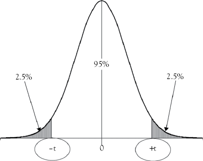
The critical values define what is known as the rejection region. For a two-tailed test, the null hypothesis is rejected if the absolute value of tc is greater than or equal to the critical t-table value at the desired confidence level. That is, tc lies in either the lower or upper shaded tail of the t-distribution.
Reconsider the data presented in Table 4.1. The values of X and Y were selected in such an arbitrary manner that you would not have any expectation about the direction of the relationship between Y and X. So, you would just be testing whether the estimated slope was indeed statistically significantly different from zero which implies that there is linear relationship between Y and X. Therefore, a two-tailed test would be appropriate. Recall that the regression equation for that data is:
![]()
The null hypothesis is that the slope is equal to zero (H0 : b = 0). The alternative hypothesis is that the slope is not equal to zero (H1 : b ≠ 0). Excel results showed that the standard error of b for this regression is 0.231, so we can calculate tc as follows:

There were 12 observations in the data set, so the number of degrees of freedom is: df = n – 2 = 12 – 2 = 10. From the t-table in Appendix 4B, find the row for 10 degrees of freedom and the column for a two-tailed test with a level of significance of 0.05, and you find the critical value for t to be 2.228 (appropriate columns for the two-tailed tests are defined along the bottom of the table in Appendix 4B). Thus, in this case the absolute value of tc (|–0.052|) is not greater than the critical table value (2.228) and you do not have enough statistical evidence to reject the null. Therefore, you conclude that there is not a statistically significant relationship between Y and X at the 5% level of significance (a = 0.05).
Applications of Cases 2 and 3
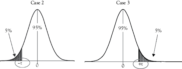
On the other hand, situations such as those described in Cases 2 and 3 call for the use of a one-tailed test because you are only trying to determine if the slope is below zero (Case 2) or above zero (Case 3). Therefore, the entire level of significance (a) goes in either the outer part of the lower tail or the upper tail of the t-distribution. This means that if you want to be 95% confident, then you would have the entire 5% significance level in the outer part of either the lower tail (Case 2) or upper tail (Case 3) of the t-distribution. The number of degrees of freedom is still equal to n – 2.
Situations described in Case 2 require the use of a left-tailed test. The null hypothesis is rejected and you conclude that the true slope is negative if tc is less than or equal to the negative critical t-table value (–t) at the desired confidence level.4 Similarly, situations described in Case 3 require the use of a right-tailed test. The null hypothesis is rejected and you conclude that the true slope is positive if tc is greater than or equal to the positive critical t-table value (+t) at the desired confidence level. The appropriate rejection region for each case is illustrated in Figure 4.3.
Now let’s check the statistical significance of the basketball WP model developed earlier. You have already determined that the model makes sense because the slope term is positive (as FG percentage increases, WP also increases). But, is the slope significantly greater than zero? This calls for a one-tailed test of the type described in Case 3. The information we need to perform the test is described in the box below:
|
The regression equation is: WP = –198.9 + 5.707(FG) n = 82 so df = 82 – 2 = 80 Computer results show that the standard error of b is: 0.783 Using a 95% confidence level (a 5% significance level) the t-table value (from Appendix 4B) is: 1.671 (Always use the row that is closest to your actual df.) H0 : β ≤ 0; slope is less than or equal to zero H1 : β > 0; slope is greater than zero |
The computed test statistic or t-ratio, tc, can be calculated as follows:

The tc (7.286) is greater than the critical t-table value (1.671). Thus, the calculated t-ratio would be out in the rejection region or shaded portion of the right-hand tail of the t-distribution and the null hypothesis is rejected. That is, at a 95% confidence level there is enough statistical evidence to show that WP is positively related to FG percentage. As a result, the slope is statistically significant!
A rule of thumb is often used in evaluating t-ratios when a t-table is not handy. The rule is that the slope term is likely to be significantly different from zero if the absolute value of the calculated t-ratio is greater than 2. This is a handy rule to remember.
Evaluation Step 3: Determine The Explanatory Power of The Model
The dependent variable (Y) used in a regression analysis will have some variability. Otherwise, there would be no reason to try to model Y. It would be convenient to have a measure of how much of that variation in Y is explained by the regression model. This is where the coefficient of determination (R2) comes in handy.
The coefficient of determination (R2) gives the percentage of the variation in the dependent variable (Y) that is explained by the regression model. The worst possible explanatory power a model could have is to explain none of the variation in the dependent variable (R2 = 0), and the best possible model would be one that explains all of the variations in the dependent variable (R2 = 1.0). Hence, the coefficient of determination (R2) will always be a value between 0 and 1. The closer it is to 0 the lower the explanatory power of the model, while the closer it is to 1 the greater is the explanatory power of the model.
For the basketball WP model the coefficient of determination is 0.399.5 This means that 39.9% of the variation in WP (the dependent variable) is explained by the model. Or you could say, 39.9% of the variation in WP is explained by variations in FG percentage (the independent variable).
Evaluation Step 4: Check For Serial Correlation
As mentioned earlier, many business and economic applications of regression analysis rely on the use of time-series data. You have already seen an example of such an application in the estimation of women’s clothing sales. When time-series data are used a problem known as serial correlation can occur.
One of the assumptions of the OLS regression model is that the error terms are normally distributed random variables with a mean of zero and a constant variance (see chapter 3). If this is true, we would not expect to find any regular pattern in the error terms. When a significant time pattern is found in the error terms, serial correlation is indicated.
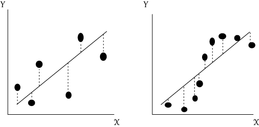
Figure 4.4 illustrates the two possible cases of serial correlation. In the left-hand graph, the case of negative serial correlation is apparent. Perfect negative serial correlation exists when a negative error is followed by a positive error, then another negative error, and so on. The error terms alternate between positive and negative values. Positive serial correlation is shown in the right-hand graph. In positive serial correlation, positive errors tend to be followed by other positive errors, while negative errors are followed by other negative errors.
When serial correlation exists, problems can develop in using and interpreting the OLS regression function. The existence of serial correlation does not bias the coefficients that are estimated, but it does make the estimates of the standard errors of b smaller than the true standard errors. This means that the t-ratios calculated for each coefficient will be overstated, which in turn may lead to the rejection of null hypotheses that should not have been rejected. That is, regression coefficients may be deemed statistically significant when indeed they are not. In addition, the existence of serial correlation causes the R2 and F-statistics to be unreliable in evaluating the overall significance of the regression function.6
There are ways to test statistically for the existence of serial correlation. The method most frequently used is the evaluation of the Durbin–Watson statistic (DW). This statistic is calculated as follows:

where et is the residual for time period t and et –1 is the residual for the preceding (t – 1) time period.7 The DW statistic will always be in the range of 0–4. As the value of the DW statistic approaches 4, the degree of negative serial correlation increases. As the value of the DW statistic approaches 0, positive serial correlation appears more severe. As a rule of thumb, a value close to 2 indicates that there is no serial correlation.
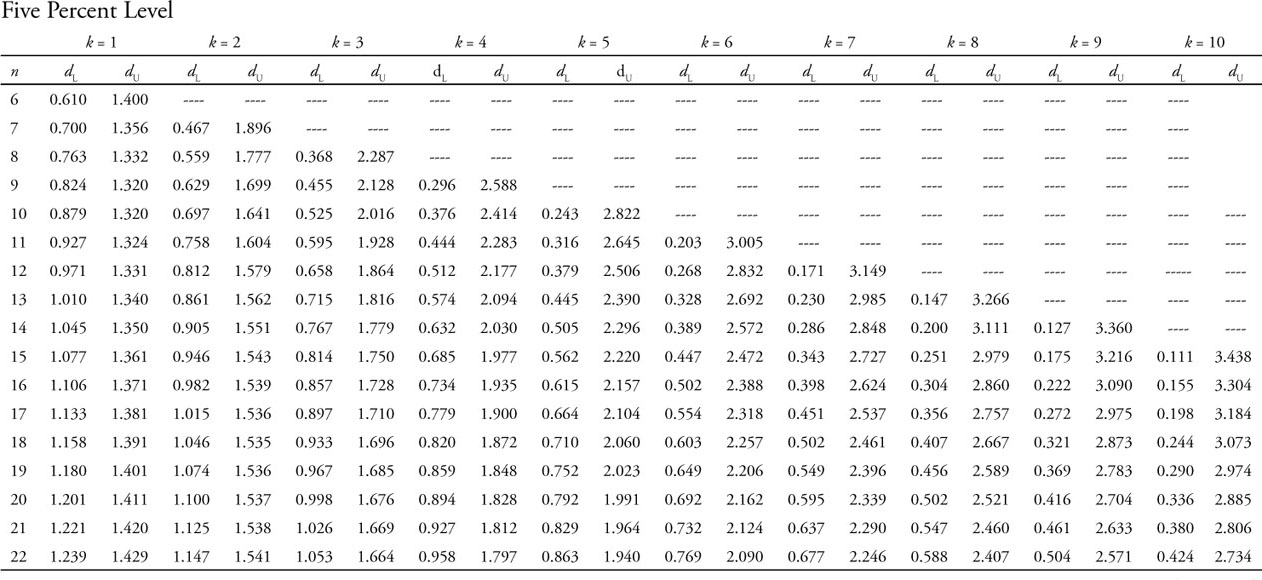
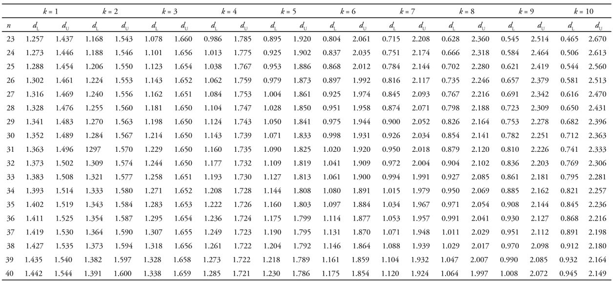
To be more precise in evaluating the significance and meaning of the calculated DW statistic, you must refer to a Durbin–Watson table (see Appendix 4C). Note that for each number of independent variables k, two columns of values labeled dl and du are given. The values in these columns for the appropriate number of observations n are used in evaluating the calculated value of DW, using the tests shown in Table 4.2. A specific example using the women’s clothing sales model can be found in Appendix 4D.
Table 4.2. Evaluating the Durbin–Watson (DW) Statistic
|
Value of the test |
Calculated DW |
Result |
|
1 |
(4 – dl) < DW < 4 |
Negative serial correlation exists |
|
2 |
(4 – du) < DW < (4 – dl) |
Result is indeterminate |
|
3 |
2 < DW < (4 – du) |
No serial correlation exists |
|
4 |
du< DW < 2 |
No serial correlation exists |
|
5 |
dl< DW < du |
Result is indeterminate |
|
6 |
0 < DW < dl |
Positive serial correlation exists |
You might wonder what causes serial correlation. A primary cause of positive serial correlation and the most common form in business/economic analysis, is the existence of long-term cycles and trends in the data. Serial correlation can also result from a misspecification of the model.
If you find a problem with serial correlation you can try several relatively simple things to reduce the problem. One is to use first differences of the variables rather than the actual values when performing the regression analysis. That is, use the change in each variable from period to period in the regression. Other potential solutions involve adding additional variables and/or nonlinear terms to the model.8
The Four-Step Evaluation Procedure: Stoke’s Lodge Occupancy Example
In chapter 1, you were introduced to a time series that represented the number of rooms occupied per month in a large independent hotel—Stoke’s Lodge. You are interested in developing and evaluating a regression model that analyzes monthly room occupancy (MRO) at Stoke’s Lodge. You think that the average gas price (GP) in dollars per gallon per month is a good predictor of occupancy. You collect a sample of monthly data from January 2002 to May 2010, which is a total of 101 observations. Table 4.3 shows a shortened section (the first 12 observations) of the data set.
Table 4.3. Monthly Data for Stoke’s Lodge Occupancy and Average Gas Price (the First Year Only)
|
Date |
Monthly room occupancy (MRO) |
Average monthly gas price (GP) |
|
Jan-02 |
6,575 |
1.35 |
|
Feb-02 |
7,614 |
1.46 |
|
Mar-02 |
7,565 |
1.55 |
|
Apr-02 |
7,940 |
1.45 |
|
May-02 |
7,713 |
1.52 |
|
Jun-02 |
9,110 |
1.81 |
|
Jul-02 |
10,408 |
1.57 |
|
Aug-02 |
9,862 |
1.45 |
|
Sep-02 |
9,718 |
1.60 |
|
Oct-02 |
8,354 |
1.57 |
|
Nov-02 |
6,442 |
1.56 |
|
Dec-02 |
6,379 |
1.46 |
The results of the bivariate regression analysis can be found in Table 4.4. The regression equation is as follows:
![]()
Step 1: Evaluate Whether the Stoke’s Lodge Model Makes Sense
One would expect there to be an inverse relationship between hotel occupancy and gas price. That is, as gas prices increase, consumers will be less likely to travel and stay in hotels. Therefore, a decrease in hotel occupancy is expected when gas prices rise. The value of the slope on gas price (GP) is indeed negative indicating that as gas price increases, hotel room occupancy (MRO) will decrease. So, the model is logical.
Step 2: Check for Statistical Significance in the Stoke’s Lodge Model
You determined that the model makes sense because the slope term is negative. But, is the slope term significantly less than zero? Since there is an expected inverse relationship between hotel room occupancy (MRO) and gas price (GP) a one-tailed test as described in Case 2 is appropriate. The null hypothesis is that the slope is greater than or equal to zero (H0 : b ≥ 0). The alternative hypothesis is that the slope is less than zero (H1 : b < 0). Excel results showed that the standard error of b for this regression is 260.702, so you can calculate tc as follows:

There were 101 observations in the data set, so the number of degrees of freedom is: df = n – 2 = 101 – 2 = 99. Then, in the t-table in Appendix 4B, find the row closest to 99 degrees of freedom (df = 120) and the column for a one-tailed test with a level of significance of 0.05, and you find the critical value for t to be 1.658. Thus, in this case the value of tc (–4.145) is less (more negative) than the negative critical table value (–1.658) and you do have enough statistical evidence to reject the null. Therefore, you conclude that there is a statistically significant negative relationship between monthly room occupancy (MRO) and gas price (GP) at the 5% level of significance (a = 0.05).
Step 3: Determine the Explanatory Power of the Stoke’s Lodge Model
For the Stoke’s Lodge model presented in Table 4.4 the coefficient of determination is 0.148. This means that 14.8% of the variation in monthly room occupancy (the dependent variable) is explained by the model. This value is relatively low. In chapters 6 and 8, you will see how this can be improved.
Table 4.4. Regression Results for Stoke’s Lodge Occupancy Simple Regression
|
Regression statistics |
||||
|
Multiple R |
0.385 |
DW = 0.691 |
|
|
|
R2 |
0.148 |
|||
|
Adjusted R2 |
0.139 |
|||
|
Standard error |
1,672.765 |
|||
|
Observations |
101 |
|||
|
| |||
|
Coefficients |
Standard error |
t Stat |
p-Value |
|
|
Intercept |
9,322.976 |
550.151 |
16.946 |
0.000 |
|
GP |
–1,080.448 |
260.702 |
–4.145 |
0.000 |
Step 4: Check for Serial Correlation in the Stoke’s Lodge Model
Since MRO is time-series data, a check for serial correlation is necessary. The DW statistic is calculated to be 0.691. To formally evaluate the DW statistic for the MRO regression you know that n = 101 (number of observations) and k = 1 (number of independent variables). From the DW table in Appendix 4C, you find the lower bound of DW = 1.442 and the upper bound of DW = 1.544. Test 6 in Table 4.2 is satisfied, since the calculated DW statistic of 0.691 is less than the lower bound (1.442) from the DW table. Therefore, positive serial correlation exists in this model. You will see that more complete models may have better results.
Summary and Looking Ahead
In this chapter, you have learned the four-step procedure used to evaluate a simple regression model. First, it is necessary to determine whether the model makes logical sense. If it does not make sense you should not continue with that particular model. Second, you should check for statistical significance of the slope term. It is necessary to determine whether a one- or two-tailed test is appropriate based on your expectations about the direction (direct, inverse, or undecided) of the relationship between Y and X. Third, you can determine the explanatory power of the model by evaluating the coefficient of determination or R-square. Finally, if you have time-series data, you need to check for serial correlation or patterns in the residuals. As you read through the rest of the book, you will use this procedure to evaluate simple regression models. Also, in chapter 6, you will learn to build on your understanding of this four-step procedure in order to evaluate multiple regression models.
What You Have Learned in Chapter 4
• To identify the four-steps involved in evaluating a simple regression model.
• To evaluate whether a simple regression model makes logical sense.
• To check for statistical significance of a slope term.
• To identify when it is appropriate to use a one-tailed versus a two-tailed hypothesis test.
• To evaluate the explanatory power of a simple regression model.
• To check for serial correlation in simple regression models with time-series data.
Appendix 4A: More Detail Concerning the Concept of “Degrees of Freedom”
The concept of “degrees of freedom” is fuzzy, to say the least. You might think of this number (df) as the number of values in the calculation of a statistic that are free to vary. The df can be determined by taking the number of individual pieces of information used to calculate a statistic (which in most cases is the total number of observations in your sample, n) minus the number of parameters that you are estimating. That is, each parameter that you are estimating costs you 1 df leaving you with fewer values that are free to vary.
If you have just two points in your regression sample data those two points determine the regression line. Neither can vary without changing the regression equation. In this case, the df would be equal to 0. You start out with two individual pieces of information (two sample data points). In order to estimate the simple regression equation Y = f (X ) = a + bX you need to estimate the values of the constant (a) and the slope (b). Each of these will cost you 1 df. If you have more than two data points all of them can vary except for two when you estimate a simple regression equation so the df = n – 2.
For multiple regression, df is defined as n – (k+1) where k is the number of independent (X) variables in the model and 1 represents the constant (a). In multiple regression, there are multiple slope terms to estimate and each of these will cost you 1 df.
The important thing for you to know is that when testing a hypothesis df comes into play. For regression df will be n – 2 or n – (k+1). Do you see that for a simple regression with one X variable the two ways to express df are equivalent?
Appendix 4B: Student’s t–Distribution
|
Level of significance for one-tailed tests |
||||
|
df |
0.10 |
0.05 |
0.025 |
0.01 |
|
1 2 3 4 5 |
3.078 1.886 1.638 1.533 1.476 |
6.314 2.920 2.353 2.132 2.015 |
12.706 4.303 3.182 2.776 2.571 |
31 821 6.965 4.541 3.747 3.365 |
|
6 7 8 9 10 |
1.440 1.415 1.397 1.383 1.372 |
1.943 1.895 1.860 1.833 1.812 |
2.447 2.365 2.306 2.262 2.228 |
3.143 2.998 2.896 2.821 2.764 |
|
11 12 13 14 15 |
1.363 1.356 1.350 1.345 1.341 |
1.796 1.782 1.771 1.761 1.753 |
2.201 2.179 2.160 2.145 2.131 |
2.718 2.681 2.650 2.624 2.602 |
|
16 17 18 19 20 |
1.337 1.333 1.330 1.328 1.325 |
1.746 1.740 1.734 1.729 1.725 |
2.120 2.110 2.101 2.093 2.086 |
2.583 2.567 2.552 2.539 2.528 |
|
21 22 23 24 25 |
1.323 1.321 1.319 1.318 1.316 |
1.721 1.717 1.714 1.711 1.708 |
2.080 2.074 2.069 2.064 2.060 |
2.518 2.508 2.500 2.492 2.485 |
|
26 27 28 29 30 |
1.315 1.314 1.313 1.311 1.310 |
1.706 1.703 1.701 1.699 1.697 |
2.056 2.052 2.048 2.045 2.042 |
2.479 2.473 2.467 2.462 2.457 |
|
40 60 120 ∞ |
1.303 1.296 1.289 1.282 |
1.684 1.671 1.658 1.645 |
2.021 2.000 1.980 1.960 |
2.423 2.390 2.358 2.326 |
|
0.20 |
0.10 |
0.05 |
0.02 |
|
|
Level of significance for two-tailed tests |
||||
Source: Modified from, NIST/SEMATECH e-Handbook of Statistical Methods, http://www.itl.nist.gov/div898/handbook/, February 6, 2012.
Appendix 4C: Critical Values for the Lower and Upper Bounds on the Distribution of the Durbin–Watson Statistic*
Appendix 4D: Calculating the Durbin–Watson Statistic in Excel
As you have learned in this chapter, the DW statistic is often used to evaluate the existence of serial correlation. Remember that serial correlation refers to patterns in the error (e) terms over time. The formula for this calculation is:

To illustrate how you can calculate the DW statistic in Excel, consider the linear regression trend for annual women’s clothing sales (AWCS) data introduced in chapter 3. The regression trend equation was: AWCS = 30,709.200 + 773.982(Year). The graph is reproduced as Figure 4D.1 and the calculation of DW statistic in Excel is shown in Table 4D.1.
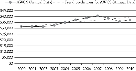
Table 4D.1. The Calculation of DW Statistic From Excel Regression Output. Note the Pattern in the Signs for the Errors
|
Residual output |
||||
|
Observation/year |
Predicted AWCS (annual data) |
Residuals = e |
(et–et–1)2 |
(et)2 |
|
1 |
31,483 |
–3.2 |
NA |
10.124 |
|
2 |
32,257 |
–770 |
588,261 |
593,152 |
|
3 |
33,031 |
–1,751 |
962,325 |
3,066,510 |
|
4 |
33,805 |
–1,207 |
295,956 |
1,457,156 |
|
5 |
34,579 |
307 |
2,292,251 |
94,182 |
|
6 |
35,353 |
1,647 |
1,795,649 |
2,712,310 |
|
7 |
36,127 |
2,589 |
887,398 |
6,702,544 |
|
8 |
36,901 |
3,436 |
717,440 |
11,805,721 |
|
9 |
37,675 |
676 |
7,617,500 |
456,927 |
|
10 |
38,449 |
–2,669 |
11,188,903 |
7,123,658 |
|
11 |
39,223 |
–2,254 |
172,240 |
5,080,516 |
|
Sums = |
26,517,923 |
39,092,687 |
||
|
DW = |
0.678 |
|||
When using Excel for regression with time-series data you want to check the box for “residuals.” Residual is another name for error (e). Errors are calculated as the actual values minus the predicted values. From that “residuals” column it is easy to use Excel to calculate DW statistic. This is shown in Table 4D.1 (parts added to the Excel output are in bold).
Remember that the ideal value for DW statistic is 2.0. Values between 2.0 and 4.0 suggest possible negative serial correlation, while values between 0.0 and 2.0 suggest possible positive serial correlation.
If you look at the graph of the regression results (Figure 4D.1) you can see that there are four negative errors, then five positive errors, and finally two more negative errors. This can also be seen in Table 4D.1, where you also see that the calculated value for DW = 0.678. This clearly represents positive serial correlation.
To formally evaluate the DW statistic for the AWCS regression trend you know that n = 11 (number of observations) and k = 1 (number of independent variables). From the DW table in Appendix 4C you find the lower bound of DW = 0.927 and the upper bound of DW= 1.324. Test 6 (see the table on the following page) is satisfied, so you know this model has positive serial correlation. You see that the calculated DW statistic of 0.678 is less than the lower bound (0.927) from the DW table.
|
Value of the test |
Calculated DW |
Result |
|
1 |
(4 – dl) < DW < 4 |
Negative serial correlation exists |
|
2 |
(4 – du) < DW < (4 – dl) |
Result is indeterminate |
|
3 |
2 < DW < (4 – du) |
No serial correlation exists |
|
4 |
du< DW < 2 |
No serial correlation exists |
|
5 |
dl< DW < du |
Result is indeterminate |
|
6 |
0 < DW < dl |
Positive serial correlation exists |
NOTES
1 If sales were measured in dollars, the slope could be either positive or negative depending on the price elasticity of demand. It would be positive for an inelastic demand and negative for an elastic demand.
2 A 95% level of confidence is common. However, 90% and 99% are also used at times.
3 For more information about degrees of freedom see Appendix 4A: More Detail Concerning the Concept of “Degrees of Freedom”.
4 Mathematically, this is the same as rejecting the null if the absolute value of the computed test statistic (| tc |) is greater than the positive critical t-table value (+t).
5 One would rarely calculate the coefficient of determination manually. It will generally be given in the computer printout and is most often identified as “R-Squared” or “R2” (in Excel it is R-Square).
7 Appendix 4D describes how to calculate the Durbin–Watson statistic in Excel.
