Figure 3.2. The ordinary least squares regression line for Y as a function of X. Residuals (or deviations or errors) between each point and the regression line are labeled ei.
The Ordinary Least Squares (OLS) Regression Model
Chapter 3 Preview
When you have completed reading this chapter you will be able to:
• Know the difference between a dependent variable and an independent variable.
• Know what portion of a regression equation (model) represents the intercept (constant) and how to interpret that value.
• Know what part of the regression equation represents the slope and how to interpret that value.
• Know that for business applications the slope is the most important part of a regression equation.
• Know the ordinary least squares (OLS) criterion for the “best” regression line.
• Know four of the basic statistical assumptions underlying regression analysis.
• Know how to perform regression analysis in Excel.
The Regression Equation
In chapter 2, you saw some examples of what is sometimes called “simple” linear regression. The term “simple” in this context means that only two variables are used in the regression. However, the mathematics and statistical foundation are not particularly simple. Two example regression equations discussed in chapter 2 are:
1. Women’s clothing sales as a function of personal income
![]()
2. Basketball WP as a function of successful FG attempt percentage
![]()
In both of these regression equations, there are just two variables. While you use Excel to get these equations, the underlying mathematics can be relatively complex and certainly time-consuming. Excel hides all those details from us and performs the calculations very quickly.
The Dependent (Y) and Independent Variables (X)
In the simplest form of regression analysis, you have only the variable you want to model (or predict) and one other variable that you hypothesize to have an influence on the variable you are modeling. The variable you are modeling (WCS or WP in the examples above) is called the dependent variable. The other variable (PI or FG) is called the independent variable. Sometimes the independent variable is called a “causal variable” because you are hypothesizing that this variable causes changes in the variable being modeled.
The dependent variable is usually represented as Y, and the independent variable is represented as X. The relationship or model you seek to find could then be expressed as:
![]()
This is called a bivariate linear regression (BLR) model because there are just two variables: Y and X. Also, because both Y and X are raised to the first power the equation is linear.
The Intercept and the Slope
In the expression above, a represents the intercept or constant term for the regression equation. The intercept is where the regression line crosses the vertical, or Y, axis. Conceptually, it is the value that the dependent variable (Y) would have if the independent variable (X) had a value of zero. In this context, a is also called the constant because no matter what value bX has a is always the same, or constant. That is, as the independent variable (X) changes there is no change in a.
The value of b tells you the slope of the regression line. The slope is the rate of change in the dependent variable for each unit change in the independent variable. Understanding that the slope term (b) is the rate of change in Y as X changes will be helpful to you in interpreting regression results. If b has a positive value, Y increases when X increases and decreases when X decreases. On the other hand, if b is negative, Y changes in the opposite direction of changes in X. The slope (b) is the most important part of the regression equation, or model, for business decisions.
The Slope and Intercept for Women’s Clothing Sales
You might think about a and b in the context of the two examples you have seen so far. First, consider the women’s clothing sales model:
![]()
In this model, a is 1,187.123 million dollars. Conceptually, this means if personal income in the United States drops to zero women’s clothing sales would be $1,187,128,000. However, from a practical perspective you realize this makes no sense. If no one has any income in the United States you would not expect to see over a billion dollars being spent on women’s clothing. Granted there is the theoretical possibility that even with no income people could draw on savings for such spending, but the reality of this happening is remote. It is equally remote that personal income would drop to zero.
Figure 2.2 is reproduced here as Figure 3.1. The line drawn through the scattergram represents the regression equation for these data. You see that the regression line would cross the Y-axis close to the intercept value of $1,187.123 if extended that far from the observed data. You also see that the origin (Y = 0 and X = 0) is very far from the observed values of the data.
The slope, or b, in the women’s clothing sales example is 0.165. This means that for every one unit increase in personal income women’s clothing sales would be estimated to increase by 0.165 units. In this example,personal income is in billions of dollars and women’s clothing sales is in millions of dollars. Therefore, a one billion dollar increase in personal income would increase women’s clothing sales by 0.165 million dollars ($165,000).
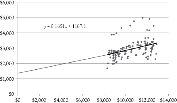
Figure 3.1. Scattergram of women’s clothing sales versus personal income. Women’s clothing sales is on the vertical (Y) axis and personal income is on the horizontal (X) axis.1
The Slope and Intercept for Basketball Winning Percentage
For the basketball WP model discussed in chapter 2, the model is:
![]()
In this example, the intercept a is negative (–198.9). Because the intercept just positions the height of the line in the graph, and because the origin is usually outside of the range of relevant data whether the intercept is positive, negative, or zero is usually of no concern. It is just a constant to be used when applying the regression model. It certainly can not be interpreted in this case that if a team had a zero success rate for FG attempts the percentage of wins would be negative.
For the slope term the interpretation is very useful. The number 5.707 tells you that for every 1% increase in the percentage of FGs that are made the team’s WP would be estimated to increase by about 5.7%. Similarly, a drop of 1% in FG would cause the WP to fall by about 5.7%. This knowledge could be very useful to a basketball coach. In later chapters, you will see how other independent variables can affect the WP of basketball teams.
How Can You Determine the Best Regression Line for Your Data?
The most commonly used criterion for the “best” regression line is that the sum of the squared vertical differences between the observed values and the estimated regression line be as small as possible. To illustrate this concept, Figure 3.2 shows five observations of the relationship between some Y variable and some X variable. You can see from the scattering of points that no straight line would go through all of the points. You would like to find the one line that does the “best” job of fitting the data. Thus, there needs to be a common and agreed upon criterion for what is best. This criterion is to minimize the sum of the squared vertical deviations of the observed values from the regression line. This is called “ordinary least squares” (OLS) regression.
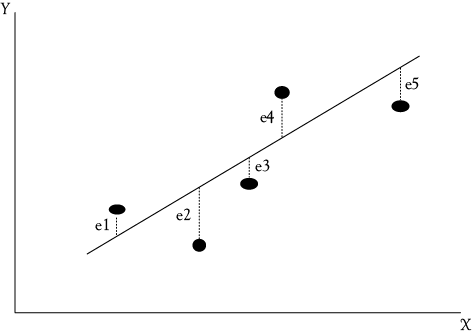
The vertical distance between each point and the regression line is called a deviation.2 Each of these deviations is indicated by ei (where the subscript i refers to the number of the observation). A regression line is drawn through the points in Figure 3.2. The deviations between the actual data points and the estimates made from the regression line are identified as e1, e2, e3, e4, and e5. Note that some of the deviations are positive (e1 and e4), while the others are negative (e2, e3, and e5). Some errors are fairly large (such as e2), while others are small (such as e3).
By our criterion, the best regression line is that line which minimizes the sum of the squares of these deviations ![]() . This regression method (OLS) is the most common type of regression. If someone says they did a regression analysis you can assume it was OLS regression unless some other method is specified. In OLS regression, the deviations are squared so that positive and negative deviations do not cancel each other out as we find their sum. The single line that gives us the smallest sum of the squared deviations from the line is the best line according to the OLS method.
. This regression method (OLS) is the most common type of regression. If someone says they did a regression analysis you can assume it was OLS regression unless some other method is specified. In OLS regression, the deviations are squared so that positive and negative deviations do not cancel each other out as we find their sum. The single line that gives us the smallest sum of the squared deviations from the line is the best line according to the OLS method.
An Example of OLS Regression Using Annual Values of Women’s Clothing Sales
The annual values for women’s clothing sales (AWCS) are shown in Table 3.1. To get a linear trend over time, you can use regression with AWCS as a function of time. Usually time is measured with an index starting at 1 for the first observation. In Table 3.1, the heading for this column is “Year.”
Table 3.1. Annual Data for Women’s Clothing Sales With Regression Trend Predictions. This Ols Model Results in Some Negative and Some Positive Errors Which Should be Expected3
|
Date |
Year |
AWCS (annual data) |
Trend predictions for AWCS (annual data) |
Error (actual– predicted) |
|
2000 |
1 |
31,480 |
31,483 |
–3 |
|
2001 |
2 |
31,487 |
32,257 |
–770 |
|
2002 |
3 |
31,280 |
33,031 |
–1,751 |
|
2003 |
4 |
32,598 |
33,805 |
–1,207 |
|
2004 |
5 |
34,886 |
34,579 |
307 |
|
2005 |
6 |
37,000 |
35,353 |
1,647 |
|
2006 |
7 |
38,716 |
36,127 |
2,589 |
|
2007 |
8 |
40,337 |
36,901 |
3,436 |
|
2008 |
9 |
38,351 |
37,675 |
676 |
|
2009 |
10 |
35,780 |
38,449 |
–2,669 |
|
2010 |
11 |
36,969 |
39,223 |
–2,254 |
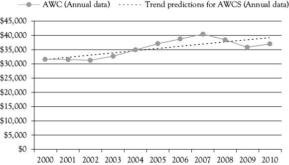
The OLS regression equation for the women’s clothing sales trend on an annual basis (AWCS) is shown in Figure 3.3. The OLS regression equation is4:
![]()
In Figure 3.3, you see that for 2000 the model is almost perfect, having a very small error and that the error is the largest for 2007. Overall, the dotted line showing the predicted values is the “best” regression line using the OLS criterion.
The Underlying Assumptions of the OLS Regression Model
There are certain mathematical assumptions that underlie the OLS regression model. To become an expert in regression you would want to know all of these, but our goal is not to make you an expert. The goal is to help you be an informed user of regression, not a statistical expert. However, there are four of these assumptions that you should be familiar with in order to appreciate both the power and the limitations of OLS regression.
The Probability Distribution of Y for Each X
First for each value of an independent variable (X) there is a probability distribution of the dependent variable (Y). Figure 3.4 shows the probability distributions of Y for two of the possible values of X (X1 and X2). The means of the probability distributions are assumed to lie on a straight line, according to the equation: Y = a + bX. In other words, the mean value of the dependent variable is assumed to be a linear function of the independent variable (note that the regression line in Figure 3.4 is directly under the peaks of the probability distributions for Y).
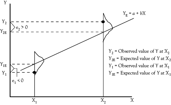
Figure 3.4. Distribution of Y values around the OLS regression line. For any X, the possible values of Y are assumed to be distributed normally around the regression line. Further, the errors or residuals (ei) are assumed to be normally distributed with a mean of zero and a constant standard deviation.
The Dispersion of Y for Each X
Second, OLS assumes that the standard deviation of each of the probability distributions is the same for all values of the independent variable (such as Xl and X2). In Figure 3.4, the “spread” of both of the probability distributions shown is the same (this characteristic of equal standard deviations is called homoscedasticity).
Values of Y are Independent of One Another
Third, the values of the dependent variable (Y) are assumed to be independent of one another. If one observation of Y lies below the mean of its probability distribution, this does not imply that the next observation will also be below the mean (or anywhere else in particular).
The Probability Distribution of Errors Follow a Normal Distribution
Fourth, the probability distributions of the errors, or residuals, are assumed to be normal. That is, the differences between the actual values of Y and the expected values (from the regression line) are normally distributed random variables with a mean of zero and a constant standard deviation.
Theory Versus Practice
These four assumptions may be viewed as the ideal to which one aspires when using regression. While these underlying assumptions of regression are sometimes violated in practice, they should be followed closely enough to ensure that estimated regression equations represent true relationships between variables. For the practitioner, it is important to note that if these four assumptions are not at least closely approximated, the resulting OLS regression analysis may be flawed. Summary statistics that are used with regression analysis allow us to check compliance with these assumptions. These statistics are described later, as are the likely outcomes of violating these assumptions.
Doing Regression in Excel
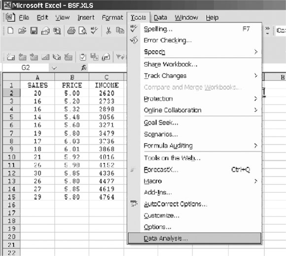
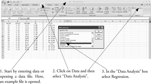
To do regression analysis in Excel, you need to use the “Data Analysis” tools of Excel. How you get to “Data Analysis” depends on the version of Excel you are using. For Excel 2003, 2007, and 2010, the instructions to get to “Data Analysis” are given at the end of chapter 1. The process of getting to “Data Analysis” is reviewed in Figure 3.5.
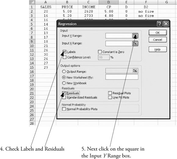
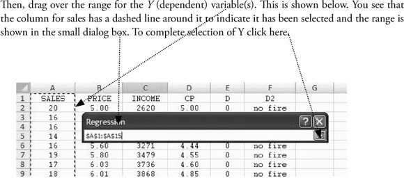
6. Next click on the square in the Input X Range box, which is right below the Input Y Range box.
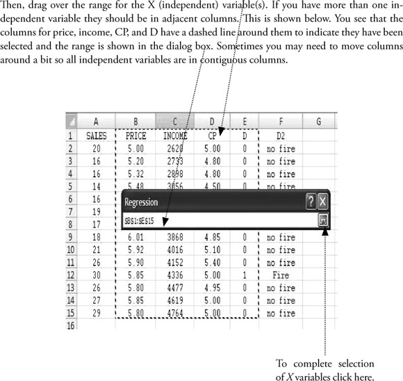
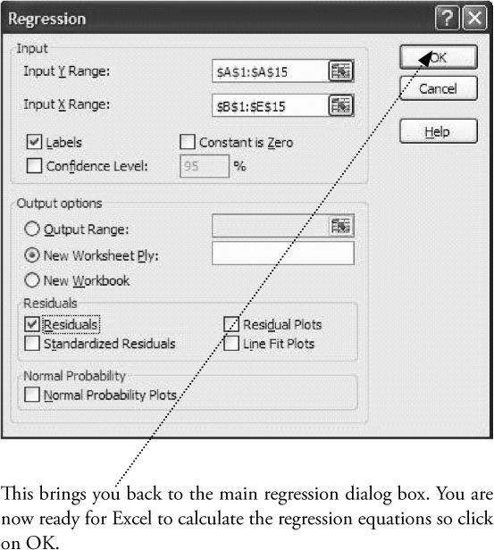
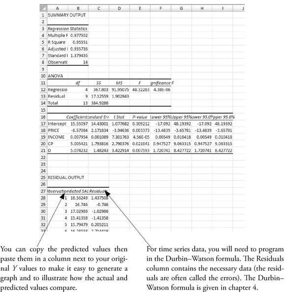
The results will appear on a new sheet, as shown below. You will probably want to delete some of this output and reformat the column widths and cells, especially reducing the number of decimal points shown.
To obtain the correlation coeffi cients for the independent variables:
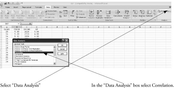
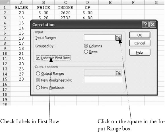
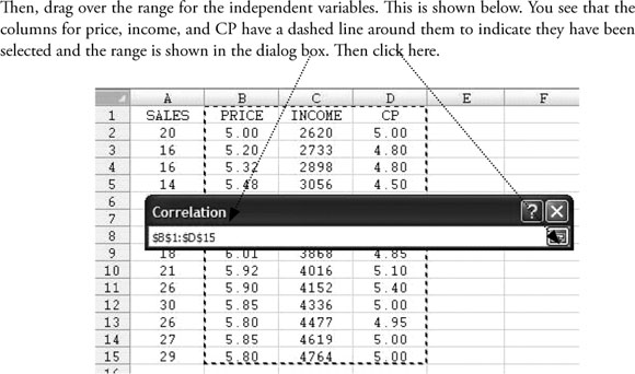
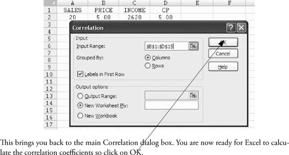
The results will appear on a new sheet, as shown below.

Once you get to the “Data Analysis” dialog box, the process of doing regression is the same in Excel 2003, 2007, and 2010. What follows is based on screen shots for 2007 but the process within “Data Analysis” will work in all three versions of Excel.
What You Have Learned in Chapter 3
• You know the difference between a dependent variable and an independent variable.
• You know what portion of a regression equation (model) represents the intercept (constant) and how to interpret that value.
• You know what part of the regression equation represents the slope and how to interpret that value.
• You know that for business applications the slope is the more important part of a regression equation.
• You know the ordinary least squares (OLS) criterion for the “best” regression line.
• You know four of the basic statistical assumptions underlying regression analysis.
• You know how to perform regression analysis in Excel.
NOTES
1 The equation written in the scattergram is the way you would get it from Excel. In this format, the slope times the independent variable is the first term and the intercept or constant is the second term. Mathematicians often use this form but the way the equation is presented in this book is far more common in practice. By comparing the two forms of the function you can see they give the same result.
2 The deviations from the regression line (ei) are also frequently called residuals or errors. You are likely to see the term residuals used in printouts from some computer programs that perform regression analysis, such as in Excel.
3 You should enter the data in Table 3.1 into Excel and use it for practice with regression. You can compare your results with those shown here.
4 This type of regression model is often called a trend regression. Some people would call the independent variable “Time” rather than “Year.”

