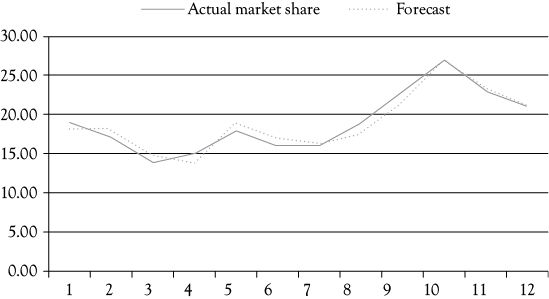
Figure 8.1. Miller’s Foods’ MS: actual and predicted with dummy variable. The line representing the estimated MS for Miller’s Foods’ is derived from the following regression model: MS = 72.908 – 7.453(P) + .017(AD) – 2.245(CAD) + 4.132(D).
Qualitative Events and Seasonality in Multiple Regression Models
Chapter 8 Preview
When you have completed reading this chapter you will be able to:
• Understand the meaning of “seasonality” in business data.
• Take seasonality into account as a pattern in your models.
• Account for seasonality by using dummy variables.
• Understand the use of dummy variables to represent a wide range of events.
• Modify the Market Share model from chapter 7 for a nonrecurring event.
• Use dummy variables to account for seasonality in women’s clothing sales.
Introduction
Most of the variables you may want to use in developing a regression model are readily measurable with values that extend over a wide range and are interval or ratio data. All of the examples you have examined so far have involved variables of this type.
However, on occasion you may want to account for the effect of some event or attribute that has only two (or a few) possible cases. It either “is” or “is not” something. It either “has” or “does not have” some attribute. Some examples include the following: a month either is or is not June; a person either is or is not a woman; in a particular time period, there either was or was not a labor disturbance; a given quarter of the year either is or is not a second quarter; a teacher either has a doctorate or does not have one; a university either does or does not offer an MBA; and so forth.
The manner in which you can account for these noninterval and non-ratio data is by using dummy variables. The term “dummy” variable refers to the fact that this class of variable “dummies,” or takes the place of, something you wish to represent that is not easily described by a more common numerical variable. A dummy variable (or several dummy variables) can be used to measure the effects of what may be qualitative attributes. A dummy variable is assigned a value of 1 or 0, depending on whether or not the particular observation has a given attribute. To explain the use of dummy variables consider two examples.
Another Look at Miller’s Foods’ Market Share Regression Model
The first example is an extension of the multiple linear regression discussed in chapter 7 dealing with a model of Miller’s Foods’ market share (MS). In that situation, you saw a regression model in which the dependent variable MS was a function of three independent variables: price (P), advertising (AD), and an index of competitors’ advertising (CAD). You saw the results of that regression in Table 7.2 and in Figure 7.1.
However, it so happens that in the second quarter of the third year (quarter 10), another major firm had a fire that significantly reduced its production and sales. As an analyst, you might suspect that this event could have influenced the MS of all firms for that period (including Miller’s Foods’). At the very least, it probably introduced some noise (error) into the data used for the regression and may have reduced the explanatory ability of the regression model.
You can use a dummy variable to account for the influence of the fire at the competitor’s facility on Miller’s Foods’ MS and to measure its effect. To do so, you simply create a new variable—call it D—that has a value of 0 for every observation except the tenth quarter and a value of 1 for the tenth quarter. The data from Table 7.1 are reproduced in Table 8.1, but now include the addition of this dummy variable in the last column.
Table 8.1. Twelve quarters (three years) of Miller’s Foods’ MS Multiple Regression Data With the Dummy Variable
|
Period |
MS |
P |
AD |
CAD |
D |
|
1 |
19 |
5.2 |
500 |
11 |
0 |
|
2 |
17 |
5.32 |
550 |
11 |
0 |
|
3 |
14 |
5.48 |
550 |
12 |
0 |
|
4 |
15 |
5.6 |
550 |
12 |
0 |
|
5 |
18 |
5.8 |
550 |
9 |
0 |
|
6 |
16 |
6.03 |
660 |
10 |
0 |
|
7 |
16 |
6.01 |
615 |
10 |
0 |
|
8 |
19 |
5.92 |
650 |
10 |
0 |
|
9 |
23 |
5.9 |
745 |
9 |
0 |
|
10 |
27 |
5.85 |
920 |
10 |
1 |
|
11 |
23 |
5.8 |
1,053 |
11 |
0 |
|
12 |
21 |
5.85 |
950 |
11 |
0 |
Using the data from Table 8.1 in a multiple regression analysis, you get the following equation for MS:
![]()
The complete regression results are shown in Table 8.2. You see that the coefficient of the dummy variable representing the fire is 4.132. The fact that it is positive indicates that when there was a fire at a major competitor’s facility, the MS of Miller’s Foods’ increased. This certainly makes sense. In addition, you can say that this event accounted for 4.132 of the 27% MS obtained during that second quarter of year 3.
Table 8.2. Miller’s Foods’ MS Regression Results Including a Dummy Variable
|
Regression statistics |
|||||
|
Multiple R |
0.970 |
DW = 1.83 |
|||
|
R-square |
0.940 |
||||
|
Adjusted R-square |
0.906 |
||||
|
Standard error |
1.183 |
||||
|
Observations |
12 |
||||
|
ANOVA |
|||||
|
|
df |
SS |
MS |
F |
Sig. F |
|
Regression |
4 |
154.202 |
38.550 |
27.541 |
0.000 |
|
Residual |
7 |
9.798 |
1.400 |
||
|
Total |
11 |
164 |
|||
|
Coefficients |
Std. error |
t Stat |
p-Value |
P/2 |
|
|
Intercept |
72.908 |
13.955 |
5.225 |
0.001 |
0.001 |
|
P |
–7.453 |
1.939 |
–3.845 |
0.006 |
0.003 |
|
AD |
0.017 |
0.002 |
7.045 |
0.000 |
0.000 |
|
CAD |
–2.245 |
0.468 |
–4.802 |
0.002 |
0.001 |
|
D |
4.132 |
1.374 |
3.008 |
0.020 |
0.010 |
You should compare these regression results with those from Table 7.2. Note particularly the following:
1. The adjusted R-squared increased from 0.812 to 0.906.
2. The standard error of the regression (SEE) fell from 1.676 to 1.183.
You see that the regression with the dummy variable is considerably better than the first model presented in chapter 7. This is further illustrated by the graph in Figure 8.1, which shows the actual MS and the MS as estimated with the multiple regression model above. Comparing Figure 8.1 with Figure 7.1 provides a good visual representation of how much the model is improved by adding the dummy variable to account for the abnormal influence in the tenth quarter.
Modeling the Seasonality of Women’s’ Clothing Sales
As a second example of the use of dummy variables, let’s look at how they can be used to account for seasonality. Table 8.3 contains data for women’s clothing sales (WCS) on a monthly basis from January 2000 to December 2011. The full series of sales, from January 2000 to March 2011, is also graphed in Figure 8.2. You see in the graph that December sales are always high due to the heavy holiday sales experienced by most retailers, while January tends to have relatively low sales (when holiday giving turns to bill paying).
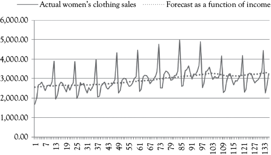
Figure 8.2. Women’s clothing sales data. Compare these two graphs to see how helpful the dummy variables for seasonality can be.
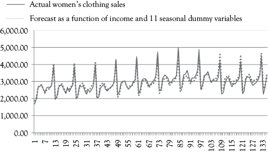
Table 8.3. Women’s Clothing Sales (in M$) and 11 Seasonal Dummy Variables. Only the First Two Years are Shown so That You See How the Dummy Variables are Set Up
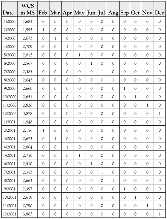
Eleven dummy variables can be used to identify and measure the seasonality in the firm’s sales. In Table 8.3, you see that for each February observation the dummy variable February has a value of 1, but March and April are 0 (as are the dummy variables representing all the remaining months). Note that for each January none of the 11 dummy variables has a value of 1. That is because the first month (i.e., January) is not February, March, or any other month. Having a dummy variable for every month other than January makes January the base month for the model.
The dummy variables for the other months will then determine how much, on average, those months vary from the first month base period. Any of the 12 months could be selected as the base. In this example, you selected the first month (January) because it is the lowest month on average after taking the upward trend in the data into account. Thus, you would expect the February, March, and April dummy variables to all have positive coefficients in the regression model.
First let’s see what happens if you just estimate a simple regression using personal income (PI) as the only independent variable. The equation that results is:
![]()
This function is plotted in the top graph of Figure 8.2 along with the raw sales data. As you can see, the estimate goes roughly through the center of the data without coming very close to any month’s actual sales on a consistent basis.
Now if you add the 11 dummy variables to the regression model, the multiple regression model that results is:

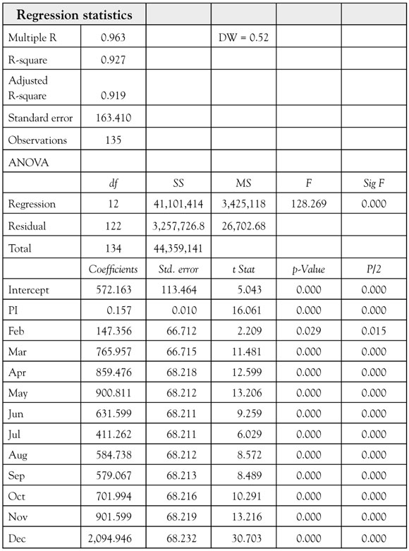
Now look at the lower graph in Figure 8.2 which shows estimated sales based on a model that includes PI and the 11 monthly dummy variables superimposed on the actual sales pattern. In many months, the estimated series performs so well that the two cannot be distinguished from one another. The complete regression results for this model are found in Table 8.4.
The interpretation of the regression coefficients for the seasonal dummy variables is straightforward. Remember that as this model is constructed, the first month (January) is the base period. Thus, the coefficients for the dummy variables can be interpreted as follows:
• For the February dummy the regression coefficient 147.36 indicates that on average February sales are $147.36 million above January (base period) sales.
• For the March dummy the regression coefficient 765.96 indicates that on average March sales are $765.96 million above January (base period) sales.
• For the April dummy the regression coefficient 859.48 indicates that on average April sales are $859.48 million above January (base period) sales.
The remaining eight dummy variables would be interpreted in the same manner.
The regression coefficient for income (0.157) means that WCS are increasing at an average of $0.157 million for every billion dollar increase in PI. Note that WCS are denominated in millions of dollars while income is denominated in billions of dollars. Knowing the units of measurement for each variable is important.
Let’s summarize some of the results of these two regression analyses of WCS:

The model that includes the dummy variables to account for seasonality is clearly the superior model based on these diagnostic measures. The better fit of the model can also be seen visually in Figure 8.2. However, the DW statistic (0.52) in the larger model does indicate the presence of positive serial correlation.
As you have seen, the development of a model such as this to account for seasonality is not difficult. Dummy variables are not only an easy way to account for seasonality; they can also be used effectively to account for many other effects that cannot be handled by ordinary continuous numeric variables.
The model for WCS can be further improved by adding two additional variables: (1) the University of Michigan Index of Consumer Sentiment (UMICS) which measures the attitude of consumers regarding the economy; and (2) the women’s unemployment rate (WUR). Both the new variables are statistically significant and have the expected signs. It should be expected that as consumer confidence climbs, sales would also increase; the positive sign on the UMICS coefficient displays this characteristic. Likewise, as women’s unemployment rises it could be expected that sales of women’s clothing would decrease; the negative sign on the WUR is consistent with this belief. These results are reported in Table 8.5; note that the adjusted R-square has increased to 0.966. This model still has positive serial correlation so you would want to be cautious about the t-tests. However, since all the t-ratios are again quite large this may not be a problem. Also, because serial correlation does not bias the coefficients these can be correctly interpreted.
Table 8.5. Regression results for WCS With the addition of the UMICS and WUR and seasonal dummy variables

In the appendix to this chapter, you will see another complete example of how dummy variables can be used to account for seasonality in data. This example expands on the analysis of occupancy for the Stoke’s Lodge model.
What You Have Learned in Chapter 8
• You understand the meaning of “seasonality” in business data.
• You can take seasonality into account as a pattern in your models.
• You know how to account for seasonality by using dummy variables.
• You understand the use of dummy variables to represent a wide range of events.
• You are able to modify the MS model from chapter 7 for a nonrecurring event.
• You can use dummy variables to account for seasonality in WCS.
AppendixStoke’s Lodge Final Regression Results
Introduction
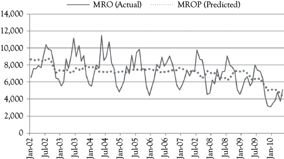
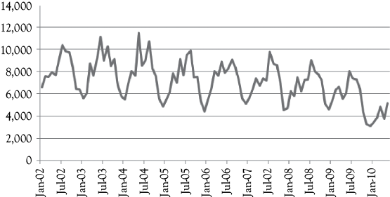
Recall that the Stoke’s Lodge MRO series represents the number of rooms occupied per month in a large independent motel. As you can see in Figure 8A.1, there is a downward trend in occupancy and what appears to be seasonality. The owners wanted to evaluate the causes for the decline. During the time period being considered there was a considerable expansion in the number of casinos in the State, most of which had integrated lodging facilities. Also, gas prices (GP) were increasing. You have seen that multiple regression can be used to evaluate the degree and significance of these factors.
The Data
The dependent variable for this multiple regression analysis is MRO. These values are shown in Figure 8A.1 for the period from January 2002 to May 2010. You see sharp peaks that probably represent seasonality in occupancy. For a hotel in this location, December would be expected to be a slow month.
Management had concerns about the effect of rising gas prices (GP) on the willingness of people to drive to this location (there is not good public, train, or air transportation available). They also had concerns about the influence that an increasing number of full service casino operations might have on their business because many of the casinos had integrated lodging facilities. Rather than use the actual number of casinos, the number of casino employees (CEs) is used to measure this influence because the casinos vary a great deal in size.
In chapter 4, you saw the following model of monthly room occupancy (MRO) as a function of gas price (GP):
![]()
You evaluated this model based on a four-step process and found it to be a pretty good model. The model was logical and statistically significant at a 95% confidence level. However, the coefficient of determination was only 14.8% (R2 = 0.148) and the model had positive serial correlation (DW = 0.691).
In chapter 6, you saw that the original model could be improved by adding the number of casino employees (CE) in the state. This yielded the following model:
![]()
This time you evaluated the model based on a five-step process because you had two independent variables rather than one, so needed to consider multicollinearity. Again the model seemed pretty good. The model was logical and statistically significant at a 95% confidence level. The coefficient of determination increased to 20.1% (Adjusted R2 = 0.201). This model also had positive serial correlation (DW = 0.730). You will see that these results can be improved by using seasonal dummy variables.
A graph of the results from the model with just two independent variables is shown in Figure 8A.2. The dotted line representing the predictions follows the general downward movement of the actual occupancy. But what do you think is missing? Why are the residuals (errors) so large for most months? Do you think it could be because the model does not address the issue of seasonality in the data? If your answer is “yes” you are right. And, as with WCS, dummy variables can be used to deal with the seasonality issue.
The Hypotheses
When you do a regression you know that you have certain hypotheses in mind. In this case you know from chapters 4 and 6 that you have the following hypotheses related to GP and CE.

That is, you have a research hypothesis that for both GP and CE the relationship with MRO is inverse. When either GP or CE increase you would expect MRO to decrease, so the alternative (research) hypothesis is that those slopes would be negative.
Based on conversations with Stoke’s Lodge management, you can expect that December is their slowest month of the year on average. You can set up dummy variables for all months except December to test to see if this is true. Thus, for the dummy variables representing January–November the hypotheses would be:

This is due to the fact that you expect all dummy variables to be positive (by construction).
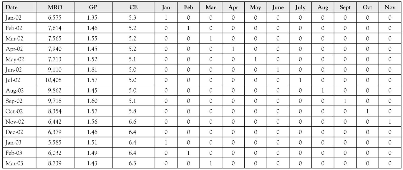
The first fifteen months of data for this situation are shown in Table 8A.1. The regression results are shown in Table 8A.2.
Table 8A.1. The First Fifteen Months of Data. Notice the Pattern of the Values for the Seasonal Dummy Variables. For Each Month in the “Date” Column There is a One in the Corresponding Column Representing that Month
The Results
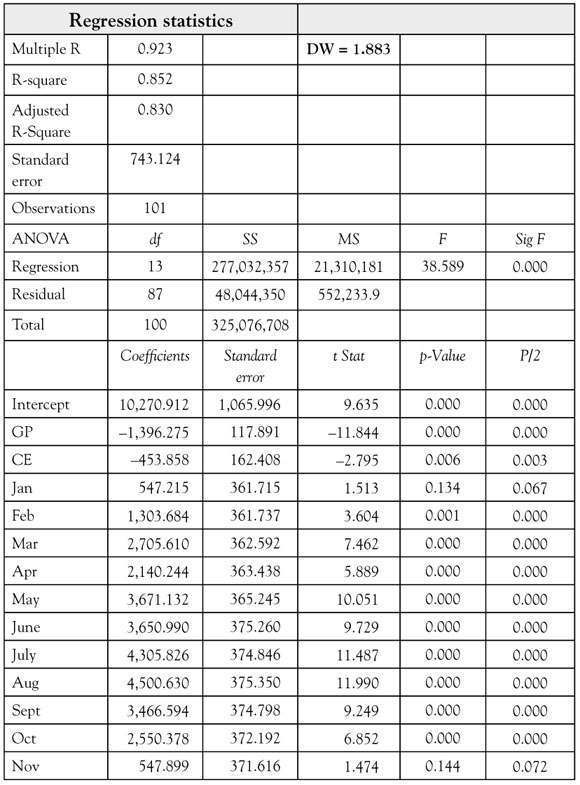
From the regression output in Table 8A.2 you see some interesting results. First, the model follows the logic you would expect with negative coefficients for CP and CE, as well as positive coefficients for all 11 seasonal dummy variables. You also see from the F-test the as a whole the regression is very significant because the significance level (p-value) for F is 0.000. This means that you can be well over 95% confident that there is a significant relationship between MRO and the 13 independent variables in the model.
The t-ratios are all large enough that p/2 is less than the desired level of significance of 0.05 except for January and November. Recall that sometimes it is reasonable for you to drop your confidence level to 90% (a significance level of 10%, or 0.10). The coefficients for January and November satisfy this less stringent requirement. Look at the “Adjusted R-square” in Table 8A.2. It is 0.830, which tells you that this model explains about 83% of the variation in MRO for Stoke’s Lodge. This is much better than the 20.1% you saw when seasonality was not considered.
In Table 8A.2, you also see that the DW statistic of 1.883 is now much closer to 2.0, the ideal value. Based on the abbreviated DW table in an appendix to chapter 4, you would be restricted to using the row for 40 observations and the column for 10 independent variables. Doing so, you would conclude that the test is indeterminate. If you look online you can find more extensive DW tables.1 For n = 100 and k = 13 you would find dl = 1.393 and du = 1.974 in which case the result is still indeterminate.
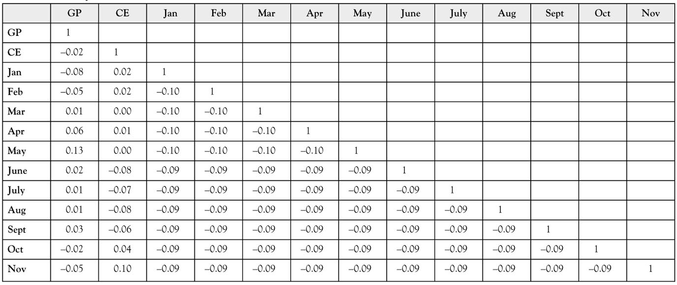
To evaluate the possibility of multicollinearity, you need to look at the correlation matrix shown in Table 8A.3. There you see that all of the correlations are quite small so there is no multicollinearity problem with this model. You may wonder why all the correlations for pairs of monthly dummy variables are not the same. This is because in the data you do not have an equal number of observations for all months. There are five more observations for January through May than for the other seven months.
Table 8A.3. The Correlation Matrix for All independent variables. All the correlation coefficients are quite small so multicollinearity is not a problem
The regression equation can be written based on the values in the “Coefficients” column in the regression results shown in Table 8A.2. The equation is:

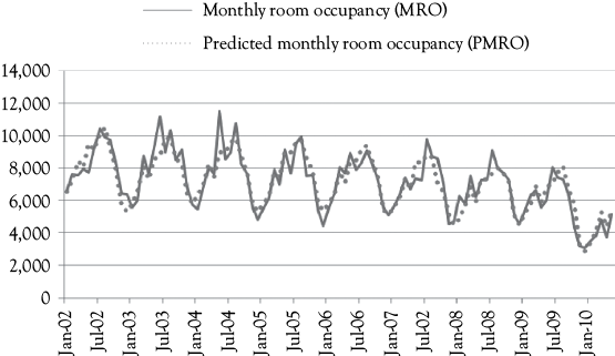
Figure 8A.3 shows you how well the predictions from this equation fit the actual occupancy data. You see visually that the fit is quite good. There are some summer peaks that appear to be underestimated. However, overall the fit is good, and certainly better than the fit shown in Figure 8A.2 for which seasonal dummy variables were not included in the model.
NOTES

