
CHAPTER 2
Elementary Time Series Techniques
Having finished reading Chapter 1, Mo decides that he has collected enough historical data to employ a quantitative forecasting method. However, he worries that he does not know any quantitative techniques. Dr. Theo assures him that this chapter will introduce the two easiest ones: simple moving averages (MA) and exponential smoothing (ES). Both of them are used to obtain one-period forecasts. As Mo has to forecast how many Honda motorcycles to order next quarter, these techniques are good starting steps for his task. Dr. Theo says that once we finish with this chapter, we will be able to:
1.Describe the four components of a time series.
2.Distinguish the MAs from the weighted moving averages (WMs).
3.Explain the ES technique.
4.Apply the Excel commands into calculating one-period forecasts.
5.Analyze and demonstrate the technique of converting nominal values to real values.
Mo looks through the chapter and sees that the section on “Components of Time Series” is easy and fun to read.
Components of Time Series
Time series data comprise trend, seasonal, cyclical, and random components.
The trend component measures the overall direction of a time series, which could have an upward, a downward, or an ambiguous moving direction (not having a trend). Figure 2.1 shows a plot of the monthly visitor arrivals by air at Honolulu.
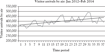
Figure 2.1 Visitor arrivals by air at Honolulu: trend component
Data Source: Department of Business, Economic Development, and Tourism: State of Hawaii (2014).
Dr. Theo reminds us that the data and Excel commands for this chapter are in the file Ch02.xls. The monthly dataset comes from Fligh, an employee of Flightime Airlines. He has carried out a research on the visitor arrivals to U.S. cities and is eager to share the information with us. This monthly dataset is available in the file Ch02.xls, Fig. 2.1, for the period from January 2011 to February 2014. The trend line reveals an upward direction in this case.
The seasonal component is the short-term movement that occurs periodically in a single year. To see this pattern more clearly, we chart the monthly data from the file Ch02.xls, Fig. 2.2, for the period from February 2012 to January 2013 and display the plot in Figure 2.2. From this figure, the peak seasons of tourists coming to Honolulu are clear. Visitor arrivals are high in December followed by the month of August. And visitor arrivals are low in April followed by the month of November.

Figure 2.2 Visitor arrivals by air at Honolulu: seasonal component
Data Source: Department of Business, Economic Development, and Tourism: State of Hawaii (2014).
The cyclical component is the long-term fluctuation that also occurs periodically, for several years and sometimes for several decades. For example, Hawaiian tourism experienced a long declining period from 1992 to 2002 without any substantial interruption. Hence, we chart yearly data from the file Ch02.xls, Fig. 2.3, for the period 1992–2013 to see a full cyclical pattern from a lowest point (the trough) to a highest point (the peak). Figure 2.3 reports the results, which reveal a full cycle of peak-to-peak from 1992 to 2006, or trough-to-trough from 2002 to 2009.
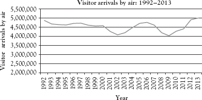
Figure 2.3 Visitor arrivals by air at Honolulu: cyclical component
Data Source: Department of Business, Economic Development, and Tourism: State of Hawaii (2014).
The random component represents the unpredictable fluctuations of any time series. They are the irregular movements resulting from shocks that affect supplies or demands in the economy. Examples of these shocks are hurricanes, earthquakes, wildfires, wars, and so on. This component is the remaining movement once the other three components, trend, seasonal, and cyclical, are factored out. Not all random movements are identifiable. However, when identification is possible, we can incorporate the randomness into our forecasts.
Dr. Theo emphasizes, “In this chapter, we assume that the seasonal and cyclical components of a dataset are not clear, that is, the time series comprises only a deterministic (with clear pattern) component and a stochastic (random movement) component. Under this assumption, forecast values can be obtained using the MA and ES techniques to smooth out any randomness in the data.”
At this point Dr. Theo reminds the class that the section on “Moving Averages” is very important because it is the basis for the later chapters. The class starts smoothly with the following section.
Moving Averages
Concept
We learn that the MA technique is the simplest in time series analyses. This technique can be used for short-term forecasts; for example, Mo has to forecast how many Honda motorcycles to order next quarter based on the historical data of the sales at his Motorland store. The technique assumes that the forecast value for the next period is an average of the previous and current-period values.
Simple MAs
The MA model assigns equal weights to past values and a current value with regard to their influences on the future values. Mathematically, a simple MA of order k can be written as:
where
| Ft+1 = | the forecast value for period (t + 1) |
| At = | the actual value for period t |
| k = | the order of the MAs |
| t = | the time period. |
At this point, Ex raises his hand and says that he does not understand why the formula has two parameters k and t in it. Dr. Theo explains that k and t are separate because k is fixed while t is moving in this formula: Each average value is formed by removing the oldest observation while adding the newest.
He then asks if any student can provide some examples. Cita says she can. Dr. Theo encourages her to go to the board, and she enthusiastically stands up. Cita offers the following discussion.
As an example, if you wish to experiment with an MA of order 3 (k = 3), and you have data for four periods, then the forecasting value for period 4 (Ft+1 = F4) is the MA of the first three periods, MA(3)3, at time period t = 3:
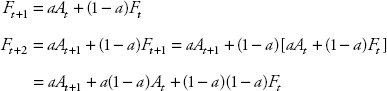
![]()
Thus, the sum in Equation 2.1 starts with:
i = t − k + 1 = 3 − 3 + 1 = 1
and ends with i = t = 3.
Cita cheerfully fills the white board with her calculations. We are all awe-struck by her mathematical skills. Cita continues:
Next, the forecasting value for period 5 (Ft +1 = F5) is the MA of the second through the fourth periods, MA(3)4, at time period t = 4:
![]()
Hence, the sum in Equation 2.1 starts with
i = t − k + 1 = 4 − 3 + 1 = 2
and ends with i = t = 4.
Ex understands now and even volunteers to go to the board to provide the class with an example from his import–export company: The actual sale values from his company in August, September, October, and November are A1 = 20, A2 = 30, A3 = 40, and A4 = 35, respectively, all in thousands of dollars. Thus, the forecasts for his company’s sales in November and December will be:
The class is very impressed with Ex’s demonstration. Dr. Theo then reminds us that a forecaster will have to experiment with several orders and perform evaluations to choose the best model with the lowest forecast errors, which will be discussed in Chapter 3. With that, we feel ready to move on, and Dr. Theo leads us to the next section.
Weighted Moving Averages
The WM technique is a little more advanced than the MA technique. A forecaster often assigns a higher weight to the more current values. The weights in the WM technique are often integers, which are assigned arbitrarily, that is, there is no limitation on the weights. Thus, Equations 2.2 and 2.3 will be transformed to the following equations:

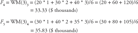
Sol remarks that in the previous example given by Ex, if we assign the weights of 1, 2, and 3 to August, September, and October, respectively, then the forecasts for his company’s sales in November and December will be:
F4 = WM(3)3 = (20 * 1 + 30 * 2 + 40 * 3)/6 = (20 + 60 + 120)/6
= 33.33 ($ thousands)
F5 = WM(3)4 = (30 * 1 + 40 * 2 + 35 * 3)/6 = (30 + 80 + 105)/6
= 35.83 ($ thousands)
Dr. Theo is very pleased, saying that her calculations are correct. He also points out that the simple MA and WM techniques in this chapter only provide one-period forecasts, and that Chapter 4 will discuss forecasting techniques that provide forecasts for two or more periods ahead. We are very excited to hear this.
Excel Applications
Dr. App starts our Excel application section with the simplest model.
Simple MA
We see that Mo is very generous to share his data with us. He also reminds us that the data and commands are in the file Ch02.xls, Fig. 2.4. Dr. App points out that Figure 2.4 displays the quarterly data on demand for Honda motorcycles from the Motorland for the period September 2011 through June 2014, the MA(3) and MA(4) values, and the forecast values using the simple MA technique. We learn that we should follow these steps to obtain the MA(3) forecasts:

Figure 2.4 Simple MA: obtaining forecast values
In cell E5, type = (D3 + D4 + D5)/3 and press Enter
Copy and paste this formula into cells E6 through E14
To obtain forecasting values Ft +1(3), copy cells E5 through E14
Right click cell F6 and select Paste Special
When the dialog box appears, select Values, then click OK
Excel will paste the values (instead of the formula) from column E into column F
The forecast value for the third quarter of 2014 using MA(3) is shown in cell F15
Repeat the same procedure for the MA(4) forecasts:
In cell G6, type = (D3 + D4 + D5 + D6)/4 and press Enter
Copy and paste this formula into cells G7 through G14
To obtain forecasting values Ft+1(4), copy cells G6 through G14
Right click cell H7 and select Paste Special
When the dialog box appears, select Values, then click OK
The forecast value for the third quarter of 2014 using MA(4) is shown in cell H15
Weighted Moving Averages
For comparative purpose, we use the same quarterly data on demand as in Figure 2.4. We find that Figure 2.5 displays the data, WM(3) values, WM(4) values, and the forecast values. The data are available in the file Ch02.xls, Fig. 2.5. To proceed with WM(3), we do the following steps:

Figure 2.5 WM: obtaining forecast values
In cell E5, type = (1 * D3 + 2 * D4 + 3 * D5)/6 and press Enter
Copy and paste this formula into cells E6 through E14
To obtain forecasting values Ft+1(3), copy cells E5 through E14
Right click cell F6 and select Paste Special
When the dialog box appears, select Values and click OK
Excel will paste the values from column E into column F
The forecast value for the third quarter of 2014 using WM(3) is shown in cell F15
For WM(4), repeat the same procedure:
In cell G6, type = (1 * D3 + 2 * D4 + 3 * D5 + 4 * D6)/10 and press Enter
Copy and paste this formula into cells G7 through G14
To obtain forecasting values Ft+1(4), copy cells G6 through G14
Right click cell H7 and select Paste Special
When the dialog box appears, select Values and click OK
The forecast value for the third quarter of 2014 using WM(4) is shown in cell H15
Dr. App concludes this section by reminding us that the Data Analysis tools in Excel has commands for MA and ES. Additionally, we can use the Math Function in Excel to calculate the average. However, she points out that one saves more time doing the techniques manually rather than using the Math Function, and a manual calculation helps us understand the concepts more clearly. We are happy to follow her advice.
Exponential Smoothing
Dr. Theo takes over the class with the next theoretical section on ES.
Concept
We learn that similar to the WM technique, the ES technique assumes that the forecast value for the next period is a weighted average of the previous and current-period values. Different from the WM, only one weight is used in ES models, and the weight is confined between zero and one. This weight is also changeable and depends on the changes in market conditions. Mathematically, the equation of forecasts using the ES model can be written as:
![]()
where Ft+1 and At are the same as in Equation 2.1
Ft is the forecast value for period t
a is the smoothing factor, also called smoothing constant (0 < a <1).
This equation states that the forecast value of period (t + 1) is equal to the weighted actual value of period t plus the weighted forecast value of period t. There are two common ways to obtain the first forecast value: calculate an average of the first several values in the actual data or take the first actual value. Montgomery, Jennings, and Kulahci (2008) also recommend a third approach of calculating an average of all values in the available data. However, this might result in a very large first value if the series moves upward sharply over time. For this reason, most textbooks take either the first value or the average of the first several values in the actual data.
Our textbook follows Hyndman and Athanasopoulos (2014), Krueger (2010), and Lawrence, Klimberg, and Lawrence (2009) in taking the first value in the actual data, that is, F1 = A1, so

Because of this gradual approach, the series does not settle until reaching period 4 and up. Also, since there is only one weight varying between zero and one, the weights assigned to past periods decrease so that the current period is given more weight. We notice the pattern of changes as follows:
Since 0 < a < 1, the weight decreases over time.
To this point, Fligh raises his hand and asks for an example. Fin volunteers to go to the board. The following is his discussion.
For example, if a = 0.2, then the weight assigned to the actual value in each period is as in the following table and continues with higher exponential orders:
| Time period | Cumulative value | Weight |
| Current period | 0.2 | 0.2 |
| One period apart | 0.2 * (1 − 0.2) | 0.16 |
| Two periods apart | 0.2 * (1 − 0.2) * (1 − 0.2) = 0.2 * (1 − 0.2)2 | 0.128 |
“Smart guy!” We exclaim. Now we know why the technique bears the name exponential smoothing.
Dr. Theo also emphasizes the advantage of using ES over WM: there is only one weight, which can be adjusted easily from zero to one, with a larger smoothing factor resulting in more weight given to the current period. For example, if a = 0.9, then the weight for the current period is 0.9, and the following weight drops sharply to 0.09.
Alte asks, “Does that means that if a = 0.1, then the weights are almost equal?” Dr. Theo commends her on the remark because in this case, the weight for the current period is 0.1, and the following weight is still 0.09, which is very close to 0.1.
Dr. Theo also reminds us that the sum of all weights over time equals to one.
At this point, Arti mentions that yesterday she read a book, in which Lawrence, Klimberg, and Lawrence (2009) offer a different way to look at the ES model by manipulating the original equation further:
![]()
The last expression (At − Ft) is the forecast error, which measures the difference between the actual value and the forecast value. In view of Equation 2.7, the ES technique provides the next-period forecast, which equals the sum of the current-period forecast and the weighted adjustment of the forecast error in the current-period forecast.
Dr. Theo is very pleased, and we find that this alternative way to look at the ES model is interesting because it shows that the ES process adjusts itself based on the forecast errors.
Rea raises his hand and suggests that we calculate the sale values from Ex’s company in the section on “Moving Averages,” again using Equation 2.5 and a calculator with the actual sales for the first three months A1 = 20, A2 = 30, and A3 = 40.
Sol asks, “So what smoothing factor should we use?” Ex says, “Let’s use the smoothing factor a = 0.5, because our company doesn’t emphasize too much on the current period but does not ignore it completely either.” Mo then adds that we should let F1 = A1 because the sales at Ex’s company increase quite rapidly over time; if we calculate the average of the three values, the initial forecast might be too large. We all think this is a good idea and work on the calculations shown in the following text.
| August: | F1 = A1 = 20 |
| September: | F2 = 0.5 * 20 + (1 − 0.5) * 20 = 20 |
| October: | F3 = 0.5 * 30 + (1 − 0.5) * 20 = 15 + 10 = 25 |
| November: | F4 = 0.5 * 40 + (1 − 0.5) * 25 = 20 + 12.5 = 32.5 |
Dr. Theo reminds us that we can verify our calculations using Equation 2.7 when we get home and to read the Excel application in the following section.
Excel Application
Dr. App starts this section by showing us Figure 2.6, which displays the data and the forecast values using the same dataset in Figures 2.4 and 2.5, setting F1 = A1, with three different smoothing factors, a = 0.3, a = 0.5, and a = 0.7. The data are in the file Ch02.xls, Fig. 2.6. We learn that we should perform the following steps to obtain the ES forecasts:

Figure 2.6 ES: obtaining forecast values
In cell E3, type = 0.3 * D2 + (1 − 0.3) * E2 and press Enter
In cell F3, type = 0.5 * D2 + (1 − 0.5) * F2 and press Enter
In cell G3, type = 0.7 * D2 + (1 − 0.7) * G2 and press Enter
Copy and paste the formulas in cells E3, F3, and G3 into cells E4 through E14, F4 through F14, and G4 through G14, respectively
Dr. App reminds us that we can experiment with Equation 2.7 using our knowledge of Excel mathematical operations learned in Chapter 1 and type the formula into corresponding cells in the dataset for Figure 2.6, and that we should be able to obtain the same results using either equation.
We then move to the next topic of transforming the data to obtain real values, which are adjusted against inflation, so that we can produce more accurate forecasts.
Nominal versus Real Values
Concept
We learn that in real life situations, some data are in quantity values that are not distorted by inflation or deflation, for example, data on building permits, quantity of books demanded, and so on. However, some data are expressed in currency values, for example, data on sales, gross domestic product (GDP), or house prices are in domestic currencies. If the values in the data are reported using different price levels for different periods (called current prices), then these values are called nominal values. The nominal values have to be converted to the real values, which are values calculated using the price level in a base period (called the constant price).
To this point, Rea asks, “Why is using real values important?” Arti offers her own experience, “Two years ago, my school made a profit of $250,000. Last year, we made $256,000. The board members and I were happy that we were growing. My accountant then pointed out to us that we were worse off because our growth rate was:
G = (256,000 − 250,000)/250,000 = 0.024 = 2.4%
However, the inflation rate during that period was 3.4 percent, so our real growth rate was 1 percent. It was a wake-up call to us. Since then, my school has been very determined to use real value in our data so that we can compensate for the inflation rate.”
“Wow, that is a good example!” We say in unison and now understand why we have to master this section.
The data conversion helps a forecaster avoid inflation and deflation distortions before applying any forecast technique. The nominal values are converted to the real values using price indexes. The two frequently used price indexes are the consumer price index (CPI) and the GDP deflator (GDPD).
Consumer Price Index
The CPI is the cost of a fixed basket of goods and services purchased by a consumer representative in the urban areas in a current year relative to the cost of the same basket in a base year. We are surprised to learn that the measurement was introduced over a century ago by the German economist and statistician, Etienne Laspeyres (1834–1913). Dr. Theo points out that the CPI measures the cost of living and so it is often used when consumer goods are examined. The equation for calculating the CPI for a current year using a base year is:

where
| CPIC = | the consumer price index for the current year |
| Qi,b = | the fixed quantity of good i in the base year |
| Pi,c = | the price of good i in the current year |
| Pi,b = | the price of good i in the base year. |
We then break into small groups to work on an example. Alte, Fligh, and I are in the same group. Here is the exercise.
Suppose the representative consumer buys a nominal value of $11,000 in consumer goods in 2014 and the real value of this basket in 2010 was $10,000, then the CPI for this basket in 2014 using 2010 as the base is:
CPI2014 = ($11,000/$10,000) * 100 = 110
Rea raises a question, “Does the result reveal that the inflation for the period 2010–2014 is 10 percent, implying an inflation rate of 2.5 percent per year on average?” Dr. Theo commends him on the correct interpretation and leads us to the next calculation: When the nominal value of $11,000 and the CPI of 110 are provided, the real value is:
Real value = ($11,000/110) * 100 = $10,000
We now know that we should use this real value to perform forecasting instead of the nominal value.
GDP Deflator
The GDPD was introduced by the German economist and statistician Hermann Paasche (1851–1925) and has been often used in macroeconomics. The index is also called the implicit price level, or the implicit GDPD. The equation for calculating the GDPD for a current year using a base year is:

where
For example, when the NGDP = $10.8 million and the GDPDC = 108, then
RGDP = ($10.8 million/108) * 100 = $10 million.
We find it is interesting to know that the GDPD has an advantage of not using a fixed basket of goods and services the way the CPI does. Hence, the disappearance of a good or appearance of a new one in a current year will be reflected in GDPD. However, the GDPD has a disadvantage of not including imported goods and imported services as the CPI does. For this reason, the GDPD usually understates the price level whereas the CPI overstates it.
At this moment, Dr. Theo asks us to give an example, and Fligh raises his hand to provide one: A hurricane destroys all oranges in Florida, so the overall price level of a few imported oranges increases sharply. Since the quantity of oranges in the CPI basket does not change, the rise in the orange price causes the CPI in Florida to go up a great deal and overstates the inflation in the state. In the meantime, the quantity of oranges is dropped from the GDPD calculation for Florida, so the total value of oranges in the GDPD is zero, and the GDPD understates the inflation in Florida.
We are truly impressed with Fligh’s intelligence. Dr. Theo is very pleased with the class and lets Dr. App work with us on the next section.
Excel Application
Ex has studied the market for exports in order to help his company and is able to provide us with the data on the exports from China to Canada. The data are in the file Ch02.xls, Fig. 2.7. We see that Figure 2.7 displays data from 2000 to 2011 in current U.S. dollars and the GDPD with 2004 as the base.
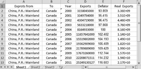
Figure 2.7 Converting nominal values to real values
Data Source: IMF.com: Direction of Trade Statistics (2014).
Since this is a macroeconomic dataset, Dr. App says that using GDPD is appropriate. We learn that to convert the nominal values to the real ones, we have to perform the following steps:
In cell F2, type = (D2/E2) * 100 and press Enter
Copy and paste the formula into cells F3 through F13
The real values are displayed in column F
Dr. App explains that a similar process can be followed to obtain real values using CPI. She also reminds us to read Chapter 3 of the textbook so that we can learn how to evaluate and adjust our forecasts in the following class.
Exercises
1.Data on the actual number of permits for residential buildings in the city are provided by Rea from Realmart and can be found in the file Real.xls. The data are from December 2012 to February 2014. Perform the WM(4) procedure on this dataset to obtain one-period forecasts with the weights of 1, 2, 3, and 4 for periods 1, 2, 3, and 4, respectively. Construct columns in Excel similar to the ones in Figure 2.5.
2.Perform the ES procedures with a = 0.4 and a = 0.6 on the dataset Real.xls to obtain one-period forecasts and construct columns in Excel similar to the ones in Figure 2.6.
3.Use the dataset Sales.xls, a handheld calculator, and the ES technique with a = 0.8 to calculate forecasts for weeks 2 through 5 of this series. Show how the steps of your calculations are similar to those in the section “Concept” under “Exponential Smoothing.”
4.The file Revenue.xls contains data on monthly revenue in current dollars for Artistown and the monthly CPI index for the city. Convert the nominal revenue values into real values.