CHAPTER 4

Intermediate Time Series Techniques

Mo comes to the class today with exciting news: His boss is very happy with the results from our combined forecasting. Additionally, his company is going to open a new branch in the south side of the city. For that reason, his boss asks him to extend the model to allow for forecasts for several periods so that they can stock up the inventory for the new branch. Ex tells us what one of his customers had asked him. “I heard that you are taking a forecasting class. Are you able to forecast your sales correctly?” For which Ex answered, “Sometimes yes, sometimes no, I guess that my forecasts are not always correct because there is a lot of uncertainty in the future.”

Dr. App assures us that this week we will discuss multiperiod forecasting and interval forecasts, which address the future uncertainty. She says that after studying this chapter, we will be able to:

1.Explain the concept of double moving averages (DMs).

2.Explain the concept of double exponential smoothing (DE).

3.Apply the concepts in (1) and (2) while calculating multiperiod forecasts.

4.Obtain interval forecasts to account for the future uncertainty.

Dr. App informs the class that Dr. Theo is still on a sick leave, so she will start our new chapter.

Double Moving Average

As the name suggests, the DM technique calculates the MAs a second time. Dr. App notifies us that for notational simplicity, the first MA henceforth is notated as M ′ while the second MA is notated as M ″.

Concept

In the DM technique, we have to calculate second MAs from the simple MAs and then combine with a trend equation to calculate the forecast values. Since we call the first MA M ′, Equation 2.1 becomes:

and the equation for second MA, M ″, is

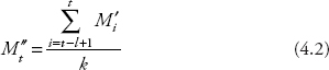
where the variable definitions are the same as those in Chapter 2 except for M ′ and M ″.

Theoretically, you can choose a different order for M ″. Empirically, the two MAs are almost always selected to have the same orders. Therefore, k is used solely to denote the order of both MAs in this textbook. For comparison, Dr. App extends the simple example in Chapter 2 with three additional periods. The new dataset is displayed in Table 4.1.

Table 4.1 Calculating M′ and M″

Period	Actual value	M′	M″
1	20
2	30
3	40	(20 + 30 + 40)/3 = 30
4	35	(30 + 40 + 35)/3 = 35
5	40	(40 + 35 + 40)/3 = 38.33	(30 + 35 + 38.33)/3 = 34.44
6	50	(35 + 40 + 50)/3 = 41.67	(35 + 38.33 + 41.67)/3 = 38.33
7	60	(40+50+60)/3 = 50	(38.33 + 41.67 + 50)/3 = 43.33

Dr. App asks Cita to go over the simple MA technique using the data in Table 4.1. She is able to provide the forecast value for period 6 as:

F_{6, MA} = M ′₅ = 38.33

Ex then volunteers to calculate the forecast error for this simple MA as follows:

The error f_{6, MA} = A₆ − F₆ = 50 − 38.33 = 11.67

We learn that the DM technique includes an equation for the trend T_t, which is written as:

so T₅ = [2/(3 − 1)] * (M₅′ − M₅″) = 1 * (38.33 − 34.44) = 3.89

At this point, Alte asks, “Dr. App, can you explain Equation 4.3 to us?”

Dr. App says, “Yes, I will explain it very soon, but I want you to have fun calculating the forecast value for period 6 with the DM technique first so that you can compare the forecast error of the F_{6, MA} with that of the F_{6, DM}. The equation for one-period forecasts using DM technique is:

where the term (M ′_t − M ″_t ) in (4.4) is the adjustment made by a forecaster upon learning of the error between the two MAs.”

Fligh volunteers to calculate the forecast for period 6 using Equation 4.4:

F_{6, DM} = 38.33 + (38.33 − 34.44) + 3.89 * 1 = 46.11

Arti then calculates the forecast error as follows:

The error f_{6, DM} = 50 − 46.11 = 3.89

We all say “Wow, this forecast error is much smaller than that of the MA.” Clearly, the DM technique can produce a better forecast model than the MA does.

Dr. App emphasizes that multiperiod forecasts are made available by using a trend line. Hence, we will calculate forecasts for period 7 and beyond after she explains the trend equation.

Trend Line in DMs

The trend is the slope of a line by definition. In the DM technique, it is the change in MAs, ΔM, over one unit change in time, Δt:

The problem is that when MAs are taken, the changes in time are often not one period, so an adjusting factor is needed. Figure 4.1 displays three groups: M′(3) and M″(3) in columns A through D, M′(4) and M″(4) in columns F through I, and M′(5) and M″(5) in columns K through N. We learn that all the data and commands for this chapter are available in the file Ch04.xls.

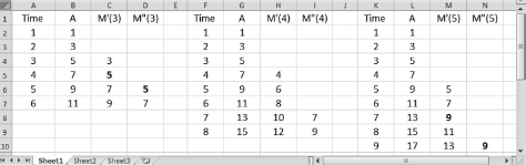
Figure 4.1 Changes in time when MAs are taken

For heuristic purpose, Dr. App uses a dataset with small values so that we can practice using a handheld calculator. Moreover, the series of the actual values has a constant slope of 2 for easy comparison. For all MAs the change in M is shown as follows:

ΔM = M ′ − M ″

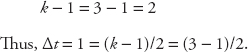
The change in time when k = 3 is exactly one period as shown in cells C5 and D6 with boldfaced numbers for easy recognition of the change. Hence, for the denominator of Equation 4.5, the time change is from period 4 to period 5, whereas the numerator is ΔM = 7 − 5 = 2. However,

Suppose you wish to use k = 5, then you are taking averages of a five-period subset and the change in time is two periods as shown in cells M8 and N10, again with boldfaced numbers to emphasize the time change from period 7 to period 9 while the numerator is:

ΔM = M ′ − M ″ = 13 − 9 = 4

and the denominator is:

Δt = 2 = (k − 1)/2 = (5 − 1)/2

When k = 4, as in columns F through I, it is a little more difficult to see because the interval falls between periods 5 and 6 where

(6 + 8)/2 = 7 = the value in cell I8.

This implies that the change in time is 1.5.

Since k = 4, we now have the denominator as

Δt = (k − 1)/2 = (4 − 1)/2 = 1.5

and the numerator is:

ΔM = M ′ − M ″ = 10 − 7 = 3.

Dr. App then says, “You should convince yourself when you get home that in any case, you always have Δt = (k − 1)/2 and that the trend equation is

Therefore, Equation 4.3 holds and implies that the trend changes from one period to the next, as long as M ′ and M ″ can be calculated.”

We all understand the trend equation now and start to calculate forecasts for the next periods.

Multiperiod Forecasts

We realize that we have already calculated the value T₅:

T₅ = [2/(3 − 1)] * (M ′₅ − M ″₅) = 1 * (38.33 − 34.44) = 3.89

So we continue by calculating the next period trends:

T₆ = 1 * (41.67 − 38.33) = 3.34

T₇ = 1 * (50 − 43.33) = 6.67

Hence, forecast values for periods 7 and 8 are

F_{7, DM} = M′₆ + (M ′₆ − M ″₆) + T₆ = 41.67 + (41.67 − 38.33) + 3.34

= 48.35

F_{8, DM} = M ′₇ + (M ′₇ − M ″₇) + T₇ = 50 + (50 − 43.33) + 6.67 = 63.34

Fin exclaims, “We have run out of trends already, T₇ is the last one!”

Dr. App smiles, “Yes, that is true. However, the trend itself can be projected into the future. For any period beyond period 8, some researchers use the last trend value (T₇ = 6.67 in the preceding example) multiplied by the number of periods ahead to be forecasted:

where m is the number of periods ahead that have to be forecasted. Since T₇ is the last trend available, we have to use T₇ and g₇(= 50 + 50 − 43.33 = 56.67) to calculate the forecast value for all later periods. For example,

However, the fact that you have many trend values also implies that you can utilize them to obtain a forecast series that mimics the market movement more closely. Here are two examples: (1) you can calculate the averages of all trend values and (2) you can calculate averages of the trend subgroups and then use them alternatively. In the preceding sample, if you calculate the average of all trend values, T_a, then

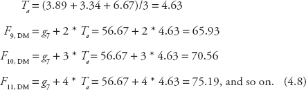
If you calculate averages of the trend subgroups with a priority given to the current trend and use the results alternatively, then the trends could be

T_a1 = (3.89 + 6.67)/2 = 5.28

T_a2 = (3.34 + 6.67)/2 = 5.01

From Table 4.1, g₆ = 41.67 + (41.67 − 38.33) = 45.01.

Hence, the forecasts will be

In brief, adding the trends enables you to forecast multiple periods ahead.”

We are relieved that we are not running out of trends. We then turn to applied exercises.

Excel Applications

Figure 4.2 displays the data from the file Ch04.xls, Fig. 4.3. We proceed with the following steps:

Figure 4.2 DM with alternative trends for multiple-period forecasts

Copy and paste the formula for simple MA in cell E4 into cells F6 through F13

In cell G6, type = 2/(3 − 1) * (E6 − F6) and press Enter

Copy and paste the formula in cell G6 into cells G7 through G13

In cell H7, type = E6 + (E6 − F6) + G6 and press Enter

Copy and paste the formula in cell H7 into cells H8 through H14 to obtain F_t+1

Regarding forecast values for the next three periods, use the last trend value:

In cell H15 type = $E$13 + ($E$13 − $F$13) + C3 * $G$13 and press Enter

(the $ signs are used to keep the same values throughout the cells. Additionally, Cell C3 is used because it has number 2 that will change into 3 and 4 in lower cells)

Copy and paste the formula in cell H15 into cells H16 and H17

To use the average of all trend values:

In cell G14, calculate the average T_a using the average command learned in Chapter 2

In cell I15, type = $E$13 + ($E$13 − $F$13) + C3 * $G$14 and press Enter

Copy and paste the formula in cell I15 into cells I16 and I17

To use the two average trends alternatively:

In cell J12, type = (G11 + G13)/2 and press Enter

In cell J13, type = (G12 + G13)/2 and press Enter

In cell J15, type = E12 + (E12 − F12) + 3 * J12 and press Enter

Copy and paste the formula in cell J15 into cell J16

In cell J17, type = E12 + (E12 − F12) + 5 * J12 and press Enter

We then construct simple plots of these series against each other. Figure 4.3 displays these plots.

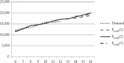
Figure 4.3 DM: plots of forecasts against actual demand

We notice that F_t+m(1) and F_t+m(2) only provide straight-line trends while F_t+m(3) mimics the small fluctuations of the actual series. All three approaches yield better results than those of simple MAs.

Ex says, “I think it is hard to tell which DM model is the best.” Dr. App replies, “That is true, so evaluations are needed. For this purpose, using hold-out sample is the best strategy if the sample for actual demand is large enough to split the historical data.” With that comment, we proceed to experiment with the holdout sample technique.

Dr. App says, “Suppose that actual data from September 2014 through June 2015 are available, we can then use data from 2011 through June 2014 for forecasting and hold data from September 2014 through June 2015 for evaluations and adjustments. This hypothetical case is illustrated in Figure 4.4, where we see that the third technique of alternating the time trend mimic the actual data most closely.”

Figure 4.4 Plots of forecasts against actual demand using holdout sample

Dr. App then encourages us to experiment with longer-term alternatives when we get home, for example, by taking the average of a three-period trend and alternating it with another three-period trend.

Double Exponential Smoothing

We learn that there are two approaches to DE: (1) Brown’s double exponential smoothing or Brown’s one-parameter double exponential smoothing, hereby called Brown’s DE, and (2) Holt’s two-parameter double exponential smoothing, hereby called Holt’s DE.

Brown’s DE

The Brown’s DE approach uses a single smoothing parameter, a, for both the smoothing and the trend equations (Brown 1963). To obtain Brown’s DE forecasts, we need to calculate the simple exponential smoothing (ES) (E ′), the second ES (E ″), and then add a trend equation. For all these calculations, the condition that 0 < a < 1 still holds.

First, we need to review the ES equation from Chapter 2. Cita volunteers to write it on the board. Arti says that she has read the section and volunteers to extend Cita’s equation to the following smoothing equations:

Fin says he has also read the section carefully and can provide the forecast equation as:

F_t+m = g_t + T_t m

where

g_t = E′_t + (E′_t − E ″_t)

T is the trend, which is written as

Dr. App is very pleased with the class’ initiative for active learning. She then asks if anyone can provide a suggestion for the initial value E′ in Equation 4.10.

Rea says he believes the initial E′ value can be calculated in multiple ways as discussed in the ES technique section in Chapter 2: (1) to take the average of a subset of the actual values, (2) to take the first value of the actual data, or (3) to follow Montgomery et al. (2008) and take the average of all values in the available data.

Dr. App praises him on his correct comment and says, “For simplicity we choose Rea’s option (2), E′₁ = A₁, and hence

E″₁ =E ′₁ = A₁ and g₁ = A₁

We will now work on an example.” We see that Table 4.2 displays calculations and forecasts for the first five periods of the data in Table 4.1 using the smoothing factor a = 0.5, E′₁ = A₁, and T₁ = 0. This demonstration can be followed using a handheld calculator. For simplicity, the calculations in this figure are rounded off to one decimal place.

Table 4.2 Brown’s DE: calculating the forecast values using a = 0.5

(1)	(2)	(3)	(4)	(5)	(6)
T	At	Et′	E″t	Tt	Ft+1
1	20	= A1 = 20	= A1 = 20	0.5/0.5 * (20 − 20) = 0
2	30	0.5 * 30 + 0.5 * 20 = 25	0.5 * 25 + 0.5 * 20 = 22.5	1 * (25 − 22.5) = 2.5	20 + 0 = 20
3	40	0.5 * 40 + 0.5 * 25 = 32.5	0.5 * 32.5 + 0.5 * 22.5 = 27.5	1 * (32.5 − 27.5) = 5	25 + 25 − 22.5 + 2.5 = 30
4	35	0.5 * 35 + 0.5 * 32.5 = 33.8	0.5 * 33.8 + 0.5 * 27.5 = 30.7	1 * (33.8 − 30.7) = 3.1	32.5 + 32.5 − 27.5 + 5 = 42.5
5	40				33.8 + 33.8 − 39.7 + 3.1 = 40

Sol points out that the value in column (3) is only E′, and the forecast value is in column (6), which is a good point as it reminds us that we are using DE instead of the ES technique.

Dr. App also mentions that it takes longer for the series to settle using DE but it will predict the market movements better than the ES thanks to the combination of the two ES calculations and the added trend.

We then move to Holt’s DE technique.

Holt’s DE

We learn that in Holt’s DE, two different smoothing parameters are used (Holt 1957). The first parameter, a, is used for the smoothing equation and can still be experimented with various factors between zero and one:

The second parameter, b, is used to smooth the trend T_t, which is calculated as:

Dr. App says that we can also try to use various factors for parameter b and that the equation for the multiperiod forecasts is quite simple:

The initial value for T can be either of the following:

where n is the number of the actual observations, or

Dr. App then asks the class to make suggestions for the initial value of E. We all guess correctly that this initial value for E can be calculated following Rea’s suggestions in the section “Brown’s DE.”

To help us understand the concept, we study Table 4.3, which displays the same dataset from Table 4.2 and shows the steps to calculate Holt’s DE. Similar to the reports in Table 4.2, the calculations in this figure are also rounded off to one decimal place.

Table 4.3 Holt’s DE: calculating the forecast values using a = 0.5 and b = 0.4

(1)	(2)	(3)	(4)	(5)
T	A	Et (a = 0.5)	Tt (b = 0.4)	Ft+1
1	20	= A1 = 20	[(30 − 20) + (35 − 40)]/2 = 2.5
2	30	0.5 * 30 + 0.5 * (20 + 2.5) = 26.3	0.4(26.3 − 20) + 0.6 * 2.5 = 4	20 + 2.5 = 22.5
3	40	0.540 + 0.5 * (26.3 + 4) = 35.2	0.4(35.2 − 26.3) + 0.6 * 4 = 6	26.3 + 4 = 30.3
4	35	0.5 * 35 + 0.5 * (35.2 + 6) = 38.1	0.4(38.1 − 35.2) + 0.6 * 6 = 4.8	35.2 + 6 = 41.2
5	40			38.1 + 4.8 = 42.9

We work on the problem using a handheld calculator and applying Equation 4.15 with the two parameters specified as a = 0.5, b = 0.4, and E₁ = A₁. We notice again that the value in column (3) is only E_t, and the forecast value is in column (5).

Dr. App says that Holt’s DE process takes even longer to settle due to its use of two different parameters.

Cita raises her hand and asks, “Does that mean that Holt’s DE technique produces better results than Brown’s DE technique?” Dr. App responds, “No, it does not necessarily work that way. Evaluations and monitoring are crucial to find the best model with the smallest error measurements, as we learned in Chapter 3.”

She then asks the class to open the Excel file and go to the applied section.

Excel Applications

We find that Figure 4.5 displays the data and calculations from the file Ch04.xls, Fig. 4.8, to obtain Brown’s DE forecasts using the smoothing factor a = 0.3 and E₁ = A₁. The following steps are needed for this exercise:

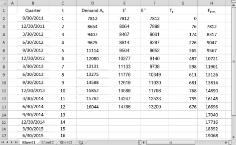
Figure 4.5 Brown’s DE with a = 0.3

In cell E3, type = 0.3 * D3 + (1 − 0.3) * E2 and press Enter

Copy and paste the formula in cell E3 into cells E4 through E13 and F3 through F13

In cell G2, type = (0.3/0.7) * (E2 − F2) and press Enter

Copy and paste the formula in cell G2 into cells G3 through G13

In cell H3, type = E2 + (E2 − F2) + G2 and press Enter

Copy and paste the formula in cell H3 into cells H4 through H14 to obtain F_t+1

To obtain F_t+m using the last period trend:

In cell H15, type =$E$13 + ($E$13 − $F$13) + C3 * $G$13 and press Enter

Copy and paste the formula in cell H15 into cells H16 and H17

For the average trend and the alternative trends, refer to the section on “Excel Applications” under “Double Moving Averages”

Suddenly, Arti exclaims, “Oh, how come the value in cell E3 of Figure 4.5 is different from that in cell E3 of Figure 2.6?”

We all look at the cells and see that she is correct.

Dr. App assures us, “Yes, the one in Figure 4.5 represents the term E′₂, which could be the forecast for period three (F₃) if you use the ES technique whereas the one in Figure 2.6 represents the forecast for period two (F₂). If you wish to scrutinize this point, you can compare the two figures and find that in Figure 4.5, the value in cell E3 is E′₂ = 8064, which equals the forecast for period three F₃ = 8064 in Figure 2.6, using the same smoothing factor a = 0.3. The forecasts of Brown’s DE are in column H.” Now it is clear to us.

We then experiment with Holt’s DE using the smoothing factor a = 0.7, b = 0.4, and E₁ = A₁. Figure 4.6 displays the data from the file Ch04.xls, Fig. 4.9, for this exercise. We learn that the following steps should be carried out:

Figure 4.6 Holt’s DE with a = 0.7 and b = 0.4

In cell E3, type = 0.7 * D3 + (1 − 0.7) * E2 and press Enter

Copy and paste the formula in cell E3 into cells E4 through E13

In cell F2, type = ((D3 − D2) + (D5 − D4))/2 and press Enter

In cell F3, type = 0.4 * (E3 − E2) + (1 − 0.4) * F2 and press Enter

Copy and paste the formula in cell F3 into cells F4 through F13

In cell G3, type = E2 + F2 and press Enter

Copy and paste the formula in cell G3 into cells G4 through G14

The forecast value for period 13 is in cell G14

To obtain F_t+m using the last period trend:

In cell G15, type= $E$13 + C3 * $F$13 and press Enter

Copy and paste the formula in cell G15 into cells G16 and G17

Dr. App then says, “You can experiment with the average trend, the alternative trends, and various smoothing factors for Brown’s DE and Holt’s DE when you get home.”

Figure 4.7 DE: plots of the forecasts against actual demand

We also chart the actual demand against Brown’s DE and Holt’s DE forecasts using the data from the file Ch04.xls, Fig. 4.10, and display them in Figure 4.7.

Dr. App concludes this section by reminding us that the holdout sample is again an appropriate strategy for evaluations in these multiperiod forecasts. She also says that Dr. Theo has recovered from his flu and is very happy to return to the class to lead us into the following section.

Interval Forecasts

Dr. Theo says that we have only learned to make point forecasts, that is, one value for each period. We learn that a point forecast does not account for the inherent fluctuation in the market. Obtaining an interval forecast will allow us to state with a certain level of confidence that the actual value will likely fall between the upper and lower bounds of this range.

Concept

Alte gives us an example from her Alcorner store. She used to buy zippers from an online source on a weekly basis. Since the shipping takes two weeks to arrive, she had to place the order on a rolling scheme: the package needed for the third week has to be ordered by the first week of a month, the package needed for the fourth week has to be ordered by the second week, and so on. Last month, she read the section on multiperiod forecasts and, based on her calculations, decided to place one large order of zippers for four weeks in place of her usual rolling scheme orders. However, by week four, she had run out of zippers and had to rush to a local store to buy them at twice the online cost. Hence, she guessed that the uncertainty is what she did not account for in her four-week forecast.

Dr. Theo thanks her for sharing her experience with us and says that she should have used interval forecasts instead of point forecasts for placing her orders. In Chapter 3, we learned that the mean absolute error (MAE) can be used to evaluate a forecast model. This same MAE can be used to construct an interval forecast. First, Equation 3.4 in Chapter 3 is for one-period MAE. For multiperiod forecasts, the uncertainty increases over time, so the simplest approximation is to adjust the MAE to MAE_t+m:

where m is the number of periods ahead to be forecasted.

The standard error of the forecast, se(f)_t+m, then can be written as:

To calculate interval forecasts, a Z-critical value of a normal distribution, Z_c, which is similar to the one we learned in Chapter 3, is given so that:

The interval is called a 100(1 − α)% confidence interval. For example, if we choose α = 0.05, then the confidence interval is 95 percent, that is, we are 95 percent confident that the actual value will fall between the upper and lower bounds of the interval.

We then break into groups to work on the problem for Alte’s store. Alte tells us the four-week forecast for Alcorner is F = 50. We follow the instruction in Chapter 3 and find that the sum of |A_t − F_t| is 96. Alte’s data contain 16 periods, but her forecast is four periods ahead, that is, m = 4. Thus, the standard error of the forecast for the fourth period is:

We decide to choose α = 0.05. Similar to the procedure in Chapter 3, α/2 = 0.025, so a normal distribution table will give Z_c = Z_(0.975) = 1.96, and the 95 percent confidence interval forecast for Alte’s store is:

50 ± 1.96 * 10 = (30.4; 69.6) ≈ (30; 70)

Thus, we are 95 percent confident that the number of zippers needed for her store will be between 30 and 70. Alte is very happy. From now on, she will make sure to order 70 zippers instead of 50 for her four-week supply.

Dr. Theo is quite pleased and says that he will continue to guide us through the next section because the Excel application is simple.

Excel Application

The interval forecasts have a lower bound and an upper bound, so we need the regions for the two tails of a normal distribution. For example, if α = 0.05, then:

α/2 = 0.025, so 1 − α/2 = 0.975.

After that, all we have to do is to type in any cell

= NORMSINV(1 − α/2) and press Enter.

For example, type

= NORMSINV(0.975) and press Enter. This yields 95 percent Z-critical value = 1.9599 ≈ 1.96.

Once the Z-critical is obtained, we can calculate the interval forecasts using the Excel mathematical operations introduced in Chapter 1.

Dr. Theo concludes the section by saying that this technique is the simplest one. In Chapters 5 and 6, we will learn more sophisticated techniques of calculating interval forecasts.

Exercises

1.The file Maui.xls contains data on visitor arrivals at Maui in Hawaii. Perform the DM(4) procedure on an Excel spreadsheet with the last trend value as the long-term trend for F_t+m up to m = 4. Construct columns in Excel similar to the ones in Figure 4.2.

2.Use the dataset Maui.xls to perform Brown’s DE procedure on an Excel spreadsheet with a = 0.7 and the long-term trend as an average of all previous trends for F_t+m up to m = 4. Construct columns in Excel similar to the ones in Figure 4.5.

3.Use a handheld calculator to perform the DM(3) on the first six observations in the dataset Sales.xls. Organize the results into a table similar to the one in Table 4.1.

4.Use a handheld calculator to perform Brown’s DE with a = 0.2 and then Holt’s DE with a = 0.2 and b = 0.7 on the first four observations in the dataset Sales.xls. Organize the results into tables similar to the ones in Tables 4.2 and 4.3.

5.The file Electricity.xls contains data on demand for electricity in Hawaii. Perform Holt’s DE on an Excel spreadsheet with a = 0.3 and b = 0.6 and with the last period trend as the long-term trend for F_{t + m} up to m = 4.

a.Construct columns in Excel similar to the ones in Figure 4.6.

b.Construct a 95 percent confidence interval for the three-period forecast (m = 3).