
CHAPTER 7
Advanced Time Series Techniques
Fligh raises a question in today’s class, “Dr. Theo, so far my boss has been satisfied with my demand forecasts for Flightime Airlines. However, he says that the holiday season is coming and that he expects high volumes of visitor arrivals by air. So he has asked me to adjust for the seasonal and cyclical effects but I don’t know how to estimate them.” Dr. Theo assures him that this week we will learn how to adjust for these two components. Some of the estimations require regression techniques learned in Chapters 5 and 6. He says that once we finish with this chapter, we will be able to:
1.Discuss the concept of decomposing a time series.
2.Analyze triple exponential technique.
3.Explain the AR(p) and ARMA/ARIMA (p, d, q) models.
4.Apply Excel while obtaining forecasts using the models learned in (1), (2), and (3).
The seasonal and cyclical components of a time series will be discussed in several sections of the chapter.
Decomposition
Dr. Theo reminds us that we were introduced to four components of a time series in Chapter 2. Each of these components now can be isolated and calculated before they are combined together to form the final forecasts.
Concept
In Chapter 6, we assume an additive model for multiple linear regressions. In this chapter, we assume a multiplicative model for decomposing a time series:
![]()
where
At = the actual data at time t
Tt = the trend component at time t
Rt = the random component at time t
St = the seasonal component at time t
Ct = the cyclical component at time t
Three-Component Decomposition
For introductory purposes, Dr. Theo first teaches us a decomposition technique that can be performed without the cyclical component similar to the one in Lawrence, Klimberg, and Lawrence (2009). The three-component model can be written as:
![]()
The decomposition process is performed in four steps:
1.Construct seasonal-random indices (SRt) for individual periods.
2.Construct a composite seasonal index (St).
3.Calculate the trend-random value (TRt) for each period.
4.Calculate the forecast values by replacing At with Ft in Equation 7.2: Ft = TRt * St.
Dr. Theo then discusses each of these four steps in detail.
Constructing Seasonal-Random Indices for Individual Periods The seasonal-random component is written as:
![]()
Equation 7.3 implies that our main task in step (1) is to obtain the de-trended data. The following technique consists of calculating a center moving average (CMA). Since data come in either quarterly or monthly, the exact center is either between the second quarter and the third quarter, or between June and July, respectively.
Suppose we have five years of quarterly data, making a total of 20 quarters. Let Q1 denote quarter 1, Q2 denote quarter 2, and so on. Then the following steps should be performed for quarterly data:
First, calculate the early moving average: EMA = (Q1 + Q2 + Q3 + Q4)/4.
Second, calculate the late moving average: LMA = (Q2 + Q3 + Q4 + Q5)/4.
Third, calculate the trend Tt = central moving average = CMA = (EMA + LMA)/2.
Finally, calculate SRt = At /Tt following Equation 7.3.
For example, data for A3, T3 for Q3, are provided, and SR3 are calculated as follows:
| Time | A3 | CMA3 = T3 | SR3 |
| Q3year1 | 64.5 | 65.8625 | 64.5/65.8625 = 0.9793 |
| Q3year2 | 59.4 | 60.3875 | 59.4/60.3875 = 0.9836 |
| Q3year3 | 70.1 | 68.85 | 70.1/68.85 = 1.0182 |
| Q3year4 | 70.8 | 70.75 | 70.8/70.75 = 1.0007 |
| Q3year5 | 72.4 | 73.0375 | 72.4/73.0375 = 0.9913 |
Ex then asks, “How about monthly data?” Dr. Theo answers, “You can analyze monthly data in the same manner, except that 12-month moving averages will be calculated.”
Constructing a Composite Seasonal Index Dr. Theo continues, “Since the seasonal-random indices are for individual quarters, and since there is some randomness in the series, an average seasonal index (AS) must be calculated.”
Dr. Theo then asks us to calculate the average seasonal index for the third quarter (AS3), and we are able to find the answer as follows:
AS3 = (0.9793 + 0.9836 + 1.0182 + 1.0007 + 0.9913)/5 ≈ 0.9946
Dr. Theo continues that 1.00 is the average index, so the sum of the four quarters must be 4.00:
AS1 + AS2 + AS3 + AS4 = 4.00
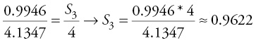
However, this is not the case most of the time due to the randomness of a time series. Hence, an adjusted average has to be calculated by scaling down all values to obtain a composite index (SQ) for each quarter, with S1 for Q1, S2 for Q2, and so on. For example, if the sum of four quarters is 4.1347, then the equation for scaling down the preceding third quarter is derived as follows:
We learn that an index lesser than 1.00 indicates a low season, and an index greater than 1.00 implies a high season. Also, some researchers multiply the index by 100 to obtain it in hundreds.
Calculating the Trend-Random Values (TRt) In the section
“Constructing Seasonal-Random Indices for Individual Periods,” we estimate each period trend so that we can divide the data by the trend to obtain the seasonal-random index. In this step, we need to obtain trend-random values by deseasonalizing the data:
![]()
Dr. Theo says that the regression technique is used for this purpose, and the econometric equation for the trend values is written as:
![]()
| where TRt = | the predicted value of the TRt line at time t |
| b1 = | the intercept of the TRt line |
| b2 = | the slope of the TRt line |
For example, suppose the regression results on the quarterly data yield this equation:
TRQ = 62.9 + 0.49 * t
Then the forecasted TRt for period 3 is:
TR3 = 62.9 + 0.49 * 3 = 64.37
Obtaining Forecast Values We learn that the forecast values can be obtained by replacing At with Ft in Equation 7.2:
![]()
For example, the composite seasonal index for Q3 is S3 = 0.9622 and the trend TR3 = 64.37, therefore:
F3 = 64.37 * 0.9622 = 61.94
Dr. Theo reminds us to note the subscript t in Equation 7.6 for Ft instead of t + 1 as in Chapters 2 through 4. In the decomposition technique, we assume that the cycle will repeat itself in the years ahead so that the calculated indices can be used to forecast for a whole new year or years ahead instead of one-period forecasts. In the preceding example, data are available up to the fourth quarter of the fifth year, so we can use the calculated indexes to obtain forecasts for the four quarters in the sixth year, the seventh year, and so on. This will become clear when we get to the section on “Excel Applications.”
Adding the Cyclical Component
Dr. Theo now adds the cyclical component, so the four-component model is:
![]()
where Ct is the cyclical component at time t.
He reminds us that calculations of the composite seasonal index SQ and time-random index TRQ are the same as earlier except that a cyclical component is assumed. Hence, we can use the same SQ and TRQ. The next step is to calculate the cyclical-random index, which can be obtained using the following equation:
![]()
Once CRt is calculated, the cyclical component C is isolated from CR (i.e., we are derandomizing the cyclical component) by calculating moving averages of the CR data to smooth out the randomness. The order of the moving average depends on the length of the business cycle. For example, if MA(5) is selected, then the results are put in the center of each five-period horizon. The values of MA(3) can be adopted for shorter cycles.
Once the cyclical component C is obtained, the random component R can be isolated:
![]()
A random index of 1.00 implies no randomness in the series. Dr. Theo reminds us that this random component is not needed to calculate the forecast values because it has been incorporated into TRt. This random component is just to show how random the time series is. Finally, forecast values are calculated using Equation 7.7 with Ft in place of At:
![]()
To conclude this theoretical section, Dr. Theo reminds us that an additive model for the decomposition technique is possible and is discussed in Gaynor and Kirkpatrick (1994).
Excel Applications
Fligh is collecting data on tourism and shares with us one of his datasets on hotel occupancy in Maui, Hawaii. The data are from the first quarter of 2008 through the second quarter of 2013 and are available in the file Ch07.xls, Fig. 7.1.

Figure 7.1 Regression results for the TRt line
Data Source: Department of Business, Economic Development, and Tourism: State of Hawaii (2014).
Dr. App tells us that it is more convenient to obtain the regression results for the TRt line first so that the steps of decomposition calculations can be grouped together in one figure.
Estimating the TRt Line
We learn that we need to perform the following steps:
Go to Data then Data Analysis, select Regression then click OK
Enter the input Y range C1:C23 and the input X range D1:D23
Check the Labels box and the button at the Output Range box
Enter F1 into the box then click OK and then OK again to overwrite the data.
Figure 7.1 displays the results of the regression with the hotel occupancy as a dependent variable and the time period as an independent variable. From this figure, you can see that the coefficient estimate of the TRt line is positive and statistically significant, implying an upward trend.
The data in this figure also reveal that the high season is in the first quarter and the low season is in the second quarter. Additionally, the hotel occupancy reached a high value of 80.9 percent in the first quarter of 2008, dropped to a trough of 56.3 percent in the second quarter of 2009, and it again rose to 80.2 percent in the first quarter of 2013. Since the seasonal pattern is clear, decomposition is the appropriate technique.
Three-Component Decomposition
Constructing Seasonal-Random Indexes for Individual Quarters (SRt) The file Ch07.xls, Fig. 7.2, shows the same quarterly data on the Maui hotel occupancy as those in the file Ch07.xls, Fig. 7.1. We must proceed as follows:
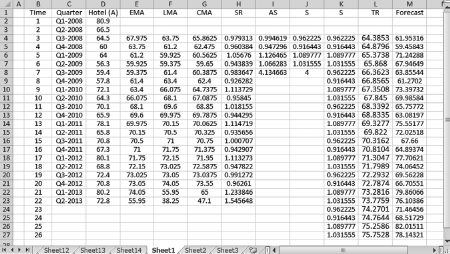
Figure 7.2 Decomposition without the cyclical componet: obtaining forecast values
In cell E4, type = (D2 + D3 + D4 + D5)/4 and press Enter
Copy and paste the formula into cells E5 through E23
In cell F4, type = (D3 + D4 + D5 + D6)/4 and press Enter
Copy and paste the formula into cells F5 through F23
In cell G4, type = (E4 + F4)/2 and press Enter
Copy and paste the formula into cells G5 through G23
In cell H4, type = D4/G4 and press Enter
Copy and paste the formula into cells H5 through H23
The seasonal-random indexes for individual quarters is displayed in column H of Figure 7.2.
Obtaining a Composite Seasonal Index (S) Cells I4 through I7 display the calculations of the average indexes ASQ, and cell I8 displays their sum. We need to perform the following steps:
In cell I4, type = (H4 + H8 + H12 + H16 + H20)/5 and press Enter
Copy and paste the formula into cells I5 through I7
In cell I8 type = SUM (I4:I7) and press Enter
In cell J4 type = I4 * 4/$I$8 and press Enter
Copy and paste the formula into cells J5 through J7
Copy and paste the formula in cell I8 into cell J8 to see that the sum is 4.00.
Copy and paste-special the values in cells J4 through J7 into cells K4 through K27
(We assume that the cycle will repeat itself in the next four quarters.)
Dr. App reminds us that the indexes in cells J4 through J7 are the composite seasonal indexes SQ. Thus, you can paste repeatedly and extend the periods to t = 26 for forecast values.
Calculating the Trend-Random Values (TRt) The TRt values are calculated by applying the regression results for the TRt line in Figure 7.1 into the 26 periods from 1 to 26. Hence,
In cell L4, type = 62.9026 + 0.49424 * B4 and press Enter
Copy and paste the formula into cells L5 through L27.
Obtaining Forecast Values (St * TRt) We learn that the following steps must be performed:
In cell M4, type = K4 * L4 and press Enter
Copy and paste the formula into cells M5 through M27.
The forecast values for the next four periods are displayed in cells M24 through M27.
Dr. App reminds us that we can extend the forecasts into the long-term future by simply extending data in columns K and L as far as you need.
Adding Cyclical Component
We find that the file Ch07.xls, Fig. 7.3, retains most of the data from the file Ch07.xls, Fig. 7.2, except for the calculations of the seasonal indexes. We proceed with this exercise as follows:

Figure 7.3 Decomposition with cyclical component: obtaing forecast values
In cell G4, type = D4/(E4 * F4) and press Enter
Paste the formula into cells G5 through G23
Copy and paste-special the values in cells G20 through G23 into cells G24 through G27
In cell H6, type = (G4 + G5 + G6 + G7 + G8)/5 and press Enter
Copy and paste the formula into cells H7 through H25
In cell I6, type = G6/H6 and press Enter
Copy and paste the formula into cells I7 through I25
(The results in column I are only used to show the randomness of the data. They are not used for forecasting)
In cell J6, type = E6 * F6 * H6 and press Enter
Copy and paste the formula into cells J7 through J25
The forecast values for the next two periods are in cells J24 and J25.
Triple Exponential Smoothing
The first approach to the triple exponential smoothing is called Holt–Winters exponential smoothing (HWE) thanks to Winters (1960) who modified the original model by Holt (1957). The HWE uses a seasonal index similar to the decomposition technique (DT). Different from the DT, the HWE adds a third equation to the existing two equations of the double exponential smoothing (DE) instead of decomposing other components of the time series.
The second approach to the triple exponential smoothing is called the higher-order exponential smoothing (HOE) because it adds a nonlinear term to the trend equation. The nonlinear term could be in quadratic, cubic, logarithmic, or any other form depending on the curvature of the series.
Concept
Holt–Winters Exponential Smoothing
This model comprises three equations with three parameters. The first parameter, a, is used to smooth out the original series:
![]()
where
L = the length of the cyclical component
S = the seasonal index
L = 4 if quarterly data are used
L = 12 if monthly data are used (Lapin 1994). The subscript (t − L) indicates that the seasonal factor is considered from L periods before period t
At this point, Arti asks, “Does that mean that the HWE uses the individual seasonal indexes instead of the composite ones?” Dr. Theo commends her for the correct observation and provides us with an example from Figure 7.3, where the actual data on hotel occupancy for the first quarter of 2012 should be divided by the seasonal index for the first quarter of 2011:
EQ1, 2012 = a(AQ1, 2012/SQ1, 2011) + (1 − a) * (EQ4, 2011 + TQ4, 2011)
The second parameter, b, is used to smooth out the trend Tt, which is the same as the one in Chapter 4:
![]()
The third parameter, c, is used to smooth out the seasonal changes:
![]()
The equation for the multiple period forecasts is:
![]()
Because the three distinct parameters are used in the three equations, this approach is also called three-parameter exponential smoothing.
Higher-Order Exponential Smoothing
This approach is appropriate when the curvature of the trend is observed. Adding a quadratic term is suitable if the curve is convex, that is, the trend rises at increasing rates over time. If the curve is concave, adding a logarithmic term is more suitable than a quadratic one.
Alte asks, “How can we know the curvature of the time series?” Dr. Theo replies, “Constructing a time series plot will help you recognize the shape of the curve and select the model.” He then says that this curve fitting processes already smooth out for the seasonal and cyclical components, so there is no need to go through the de-seasoning and de-randomizing processes as in decomposition technique. Thus, the forecast model with a quadratic term added is:
![]()
| where Ft+1 = | the forecasted value of the series at time (t + 1) |
| b1 = | the intercept of the trend curve = the initial value of the actual data |
| b2 = | the slope of the linear trend |
| b3 = | the slope of the nonlinear trend |
If the trend equation is extended to allow a logarithmic term, then Equation 7.15 becomes:
![]()
In Equations 7.15 and 7.16, there are a total of three parameters to be estimated, so the technique is also called the triple exponential or three-parameter exponential smoothing technique. We learn that estimating Equation 7.15 or Equation 7.16 to obtain the three parameters and the predicted values in one regression is the best approach of forecasting.
Dr. Theo tells us that researchers also try higher-order polynomial models (Brown 1963; Montgomery, Jennings, and Kulahci 2008) and hence we have the name higher-order exponential smoothing.
Excel Applications
Holt–Winters Exponential Smoothing
The file Ch07.xls, Fig. 7.4, displays the same data from Fligh as those in the file Ch07.xls, Fig. 7.2, and the calculations using the smoothing factors a = 0.4, b = 0.6, and c = 0.7. The data are on hotel occupancy in Maui, Hawaii from the first quarter of 2008 through the second quarter of 2013. The initial exponential smoothing value is chosen as the first actual value, and the first trend value is calculated by averaging the first two trend values. We learn to proceed as follows:
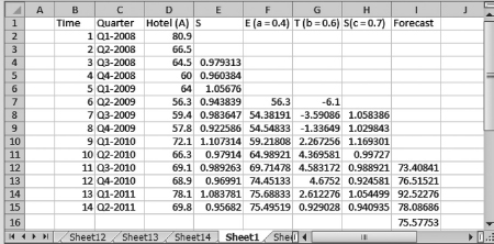
Figure 7.4 Holt-Winters exponential smoothing: obtaining forecast values
In cell G7, type = ((D7 − D6) + (D5 − D4))/2, then press Enter
In cell F8, type = 0.4 * (D8/E4) + 0.6 * (F7 + G7), then press Enter
Copy and paste the formula into cells F9 through F15
In cell G8, type = 0.6 * (F8 − F7) + 0.4 * G7, then press Enter
Copy and paste the formula into cells G9 through G15
In cell H8, type = 0.7 * (D8/F8) + 0.3 * E4, then press Enter
Copy and paste the formula into cells H9 through H15
In cell I12, type = (F11 + G11) * H8, then press Enter
Copy and paste the formula into cells I13 through I16
The one period forecast is in cell J16
For multiperiod forecasts, follow the same alternative procedures as those in Chapter 4. The advantage of the HWE is that it can be used for data that exhibit seasonal patterns in addition to the two deterministic and random components as in moving average and DE techniques.
Higher-Order Exponential Smoothing
Cita is doing research on the behavior of the firms and shares with us data on labor force from the Department of Business, Economic Development, and Tourism in Hawaii. Data are for the first quarter of 2006 through the second quarter of 2013 and are available in the file Ch07.xls, Fig. 7.5. To select an appropriate model for regression, we need to construct a time series plot. Figure 7.5 displays this plot, which shows a concave curve and implies that adding a logarithmic trend to the forecast model appears to be the best strategy.

Figure 7.5 Selecting regression model: time series plot
Data Source: Department of Business, Economic Development, and Tourism: State of Hawaii (2014).
Hence, the econometric model is written as:
LABORt+1 = b1 + b2 TIMEt + b3 ln(TIMEt) + et+1
We learn to perform the following steps with the data in the file Ch07.xls, Fig. 7.6:
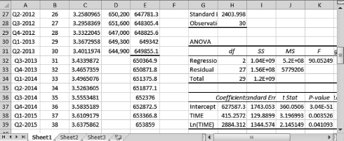
Figure 7.6 Higher-order exponential smoothing: obtaining forecast values
Go to Data then Data Analysis, select Regression and click OK
The input Y range is D1:D31, the input X range is B1:C31
Check the boxes Labels and Residuals
Check the button Output Range and enter G21 then click OK
(We place the results into cell G21 to make the next steps of calculations convenient)
A dialogue box will appear, click OK to overwrite the data
Dr. App reminds us to click on Residuals so that predicted values are reported in the Excel results. Sections of the regression results and data (from time period t = 26 through t = 30) are displayed in Figure 7.6. We also notice that the actual and predicted values from Excel results end at period t = 30, where a dark line marks the end in cell E31. The advantage of this approach is that multiperiod forecasts can be easily obtained. The values in cells E32 through E39 are multiperiod forecasts. To proceed with this exercise, we must follow these steps:
Copy and paste the formula in cell C31 into cells C32 through C39
In cell E32, type = $H$37 + $H$38 * B32 + $H$39 * C32, then press Enter
Copy and paste this formula into cells E33 through E39
Dr. App reminds us that we can extend the forecasts as far as we wish into the future. The results from Figure 7.6 also confirm our intuition that a combination of a logarithmic trend and linear trend is suitable for this time series: coefficient estimates of both variables are statistically significant with p-values of TIME and ln(TIME) equal 0.0035 and 0.041, respectively.
Dr. Theo says that sometimes our selection of a model might not be suitable. If the model is not statistically significant, then we will need adjustments as discussed in Chapters 5.
A Brief Introduction to AR and ARIMA Models
The name ARIMA sounds so pretty that we are curious to learn about the model. The autoregressive (AR) and autoregressive integrated moving average (ARIMA) models belong to time series analyses instead of associative analyses because they involve only the dependent variable and its own lags instead of an outside explanatory variable.
Concept
AR and ARIMA models explore the characteristics of a time series dataset that often has the current value correlated with its lagged values and can be used for multiple period forecasts.
AR models
A dependent variable in an AR model can contain numerous lags. The model is denoted as AR(p), where p is the number of lags. When a dependent variable is correlated to its first lag only, the model is called an autoregressive model of order one and is denoted as AR(1):
![]()
If |a| < 1, then the series is stationary because the series gradually approaches zero when t approaches infinity. When |a| ≥ 1, the series is nonstationary: If a >1, then the series explodes when t approaches infinity. If |a| = 1, the series is said to follow a random walk because it is wandering aimlessly upward and downward with no real pattern:
![]()
At this point, Ex asks, “Why is the process called a random walk?” Fin raises his hand and offers a story to explain the concept, “A drunken man behind the wheel was stopped by a police officer, who then asked him to walk a straight line. Of course the man could not do it. He just wandered aimlessly one step to the right, one step to the left, going forward one step, and then going backward one step. Hence, the best you can guess of his next step is to look at his previous step and add some random error to it. This is exactly what we see in Equation 7.18.”
Dr. Theo thanks Fin for the fun story and says that et is assumed to be independent with a mean of zero and a constant variance. He then continues, “If all lagged variables are stationary as in Equation 7.17, regressions using OLS can be performed, and multiple period forecasts can be obtained by the same recursive principle discussed in Chapter 6. For example, a model with a constant and two lagged values can be estimated as:
![]() t = â1 + â2 yt−1 + â3 yt−2
t = â1 + â2 yt−1 + â3 yt−2
![]() t+1 = â1 + â2
t+1 = â1 + â2 ![]() t + â3 yt−1
t + â3 yt−1
![]() t+2 = â1 + â2
t+2 = â1 + â2 ![]() t+1 + â3
t+1 + â3 ![]() t
t
Hence, long-term forecasts can be obtained in a very convenient manner.”
Point Forecasts
We then break into groups to work on the following example. Estimating a stationary AR(2) model of Galaxy phone sales from a telephone shop in our city gives the following results:
SALEt = 0.54 SALEt−1 + 0.48 SALEt−2
Sale values are known as SALEt = $4800 and SALEt−1 = $4700. Thus:

Dr. Theo tells us that when a series follows a random walk, we might obtain significant regression results from completely unrelated data, which is called a spurious regression. He assures us that if one of the lagged variables has unit coefficient (ak = 1), taking the first difference of the equation can turn it into a stationary series. For example, taking the first difference of Equation 7.18 yields a first differencing model:
![]()
Δyt is a stationary series because et is an independent random variable with a mean of zero and a constant variance. Any series that can be made stationary by taking the first difference is said to be integrated of order one and is denoted as an I(1). Any series similar to Δyt is said to be integrated of order zero and is denoted as an I(0). This characteristic can be applied in forecasting an AR(p) model, in which (p − 1) series are stationary. For example, an AR(3) model that has the first lagged series nonstationary is as follows:
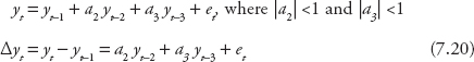
Estimation can be performed on Equation 7.20 using the OLS technique. Once coefficient estimates are obtained, the predicted value of Δyt can be calculated. Since yt−1 is known, yt can be calculated, which allows for multiperiod forecasts.
We then work on the next example. A restaurant estimates this equation for its sale values:
ΔSALEt = SALEt − SALEt−1 = 0.12 SALEt−2 + 0.08 SALEt−3
Sale values are known as SALEt = $4200, SALEt−1 = $4100, and SALEt−2 = $4000. Hence:

Dr. Theo then reminds us that the first differenced model can be extended to panel data. The suitable case for using first differencing in panel data is that the error term follows a random walk (Wooldridge 2013). In this case, taking the first difference serves two purposes: (i) to eliminate the intercept a1i presented in Equation 6.24, and (ii) to make Δe become an I(0):

Interval Forecasts
The formula for the standard error of the regression, s, in AR(p) models is still the same:

However, the formulas for the standard error of the forecast, se(f), can be calculated in a more precise manner than the ones in the previous chapters and are shown in Hill, Griffiths, and Lim (2011):

For AR(1) models, the first two se(f) values are the same as in Equation 7.22, but the se(f) for the interval forecasts can be extended into m periods ahead as shown in Griffiths, Hill, and Judge (1993):
![]()
As an example, suppose that SSE = 1260 and T = 40. The point forecasts from the previous example are:
SALEt+1 = 0.54 SALEt + 0.48 SALEt−1 = 0.54 * 4800 + 0.48 * 4700 = 4848
SALEt+2 = 0.54 SALEt+1 + 0.48 SALEt = 0.54 * 4848 + 0.48 * 4800 ≈ 4922
SALEt+3 = 0.54 SALEt+2 + 0.48 SALEt+1 = 0.54 * 4922 + 0.48 * 4848 ≈ 4985
The standard errors of the forecast errors are:

![]()

![]()
Thus, the interval forecasts for a 95 percent confidence interval are:
SALEt+1 = 4848 ± 5.7583 * 2.024 = (4836; 4860)
SALEt+2 = 4922 ± 6.5442 * 2.024 = (4909; 4935)
SALEt+3 = 4985 ± 7.91 * 2.024 = (4969; 5001)
ARMA versus ARIMA
When a dependent variable is correlated to a lagged value of its errors, the model is called a moving average of order one and is denoted as MA(1):
![]()
Combining an AR(1) and an MA(1) gives an ARMA(1, 1) model:
![]()
If the series can be made stationary by taking the first difference, the ARMA(1, 1) becomes an ARIMA(1, 1, 1), where the letter I in the middle of ARIMA stands for integrated of order one.
The model can have any order. Hence, a general ARIMA model can be written as an ARIMA (p, d, q), where p is the order of autoregressive, d is the order of integration (differencing), and q is the order of moving average. Once an ARIMA model is specified, the value for period (t + 1) can be forecasted by substituting the value for period t into Equation 7.17 or Equation 7.18 and continue for the subsequent periods using the recursive principle.
For choosing p and q in the ARIMA (p, d, q) model, a model search process called Box–Jenkins procedure is often followed. The Box–Jenkins procedure consists of three steps. The first step is the model identification, in which a model is derived based on economic theories. The second step is the estimation, in which regressions are performed. The third step is the diagnostic checking, in which tests are carried out and residual plots are produced to evaluate the robustness of the model. The procedure is then repeated until the best model is obtained.
To conclude the section, Dr. Theo says that the topic of ARIMA models requires an in-depth knowledge of time series analysis and is beyond the scope of this textbook. He encourages us to read a book written specifically for time series modeling if we are interested in ARIMA models and the Box–Jenkins procedure.
Testing for Stationarity
We learn that the test is called the Dickey–Fuller test or unit-root test because a series is stationary if a < 1. The null hypothesis is that y is nonstationary. The calculations of the statistic values are the same as those of the t-statistics. However, when y is nonstationary, the variance of y is inflated and so the distribution is no longer a t-distribution but follows a τ (tau) distribution. The statistic is therefore called τ-statistic (tau-statistic). The original equation to derive the test is:
yt = ayt−1 + et
Subtracting yt−1 from both sides yields:
yt − yt−1 = (a − 1) yt−1 + et
Δyt = c yt−1 + et
where
![]()
If a = 1 then c = 0, so Equation 7.26 is very convenient to test because t-statistics in all quantitative packages are for a test of significance with the null hypothesis for c = 0. The four steps of the Dickey–Fuller test are similar to those in Chapter 5 with the hypotheses:
H0: c = 0; Ha: c < 0
To perform the Dickey–Fuller test, the model in Equation 7.26 is often extended to allow for a constant term and a trend. The model with the constant term is:
![]()
The model that adds the trend is:
![]()
Dr. Theo says that these three models are usually estimated concurrently so that the most appropriate model is selected based on whether or not the constant term or the trend is significant. The τ-critical values for Dickey–Fuller tests are organized into tables that are three pages long in Fuller (1976, 371–3). For instructional purposes, Table 7.1 displays the most important ones based on OLS estimates for large samples and are reformatted to fit the preceding models.
Table 7.1 Critical values for Dickey–Fuller τ distribution
| Significance Level | 0.01 | 0.025 | 0.05 | 0.10 |
| For model (7.26) | −2.58 | −2.23 | −1.95 | −1.62 |
| For model (7.27) | −3.43 | −3.12 | −2.86 | −2.57 |
| For model (7.28) | –3.96 | −3.66 | −3.41 | −3.12 |
Source: Adapted from Fuller (1976, 373).
Since τ-statistics have the same values as t-statistics, you can look for the standard errors from Excel Summary Outputs and calculate the t-statistics using the same formula for those in Chapter 5. Hence, the four standard steps of the Dickey–Fuller tests are as follows.
ii.Calculate τ-statistics = t-statistics.
iii.Find τ-critical.
iv.Decision: If |τ-statistics| > |τ-critical| (or τ-statistics < τ-critical), we reject H0, meaning c < 0, implying the model is stationary.
Dr. Theo reminds us that we can extend the preceding models to allow more lags and still use the critical values listed in Table 7.1.
Excel Applications
Dr. App starts this section by informing us that we will need special statistical packages to perform estimations and obtain forecasts with ARIMA (p, d, q) models. Hence, she only provides demonstrations for the AR(p) model in the following section.
Sol is doing research on the effect of the solar energy on electricity companies. She shares with us a monthly dataset on the sales of electricity for commercial facilities in Kauai from the Department of Business, Economic Development and Tourism in Hawaii. The data are available in the file Ch07.xls, Fig. 7.8.
Testing Stationarity
We first estimate Equation 7.26 by regressing ΔELECTt on ELECTt−1 without a constant term:
Go to Data then Data Analysis, select Regression and click OK
The input Y range is E1:E99, the input X range is D1:D99
Check the boxes Labels and Constant is Zero
Check the button Output Range and enter I1 and click OK
Click OK again to overwrite the data
We learn that Figure 7.7 displays coefficient estimates and their t-statistics for the three regressions of Equations 7.26, 7.27, and 7.28. Panel 7.8a is for Equation 7.26. Panels 7.8b and 7.8c are for Equations 7.27 and 7.28, respectively. We then continue with the second regression of ΔELECTt on ELECTt−1 for Equation 7.27, which has the constant term added to the model:

Figure 7.7 Regression results for the Dickey–Fuller tests
Data Source: Department of Business, Economic Development, and Tourism: State of Hawaii (2014).
Go to Data then Data Analysis, select Regression and click OK
The input Y range is E1:E99, the input X range is D1:D99
Check the box Labels (this time do not check on the box Constant is Zero)
Check the button Output Range and enter N1 and click OK
Click OK again to overwrite the data and obtain the results in Panel 7.8b
Finally, we perform the third regression of ΔELECTt on ELECTt−1 and TIME for Equation 7.28:
Go to Data then Data Analysis, select Regression and click OK
The input Y range is E1:E99, the input X range is C1:D99
Check the box Labels
Check the button Output Range and enter S1 and click OK
Click OK to overwrite the data and obtain the results in Panel 7.8c
From the results in Panel 7.8a, the null hypothesis is not rejected, implying that the model is not stationary. From the results in Panel 7.8b and 7.8c, the null hypotheses are rejected for the second and the third models, implying the stationarity of each model. Panel 7.8c also shows that the trend is significant. Hence, forecasting should be performed using the third model in Panel 7.8c.
Forecasting with AR Models
Since we choose Equation(7.28), of which the results are displayed in Panel 7.8c, using the recursive principle to project one period forward yields:
ΔELECTt+1 = 9,533,512 − 10082 TIME − 0.3889 ELECTt
The data shows that ELECTFeb-06 = 21,761,678, so

To obtain the multiperiod forecasts in Excel, we must perform the following steps:
In cell F3, type = 9533512 − 10082 * C2 − 0.3889 * B2 and press Enter
(Alternatively, you can enter the cell numbers in cells T17, T18, and T19, respectively)
In cell G3, type = B2 + F3 and press Enter
In cell F4, type = 9533512 − 10082 * C3 − 0.3889 * G3
Copy and paste the formula into cells F5 through F103
(Ignore the values at this moment, as the formula in cell G4 needs to be adjusted)
In cell G4 type = G3 + F4
Copy and paste the formula into cells G4 through G103 for multiperiod forecast
Dr. App concludes, “You can extend the forecasts into long-term future by extending columns F and G. You can also obtain the interval forecasts by typing the formulas in the section on “Concept” under “A Brief Introduction to AR and ARIMA Models” in any Excel cells using the mathematical operations learned throughout this book. However, a handheld calculator is doing just as well and so no Excel application is introduced for interval forecasts.”
Exercises
1.The file Hawaii.xls contains data on the number of visitor arrivals to the Big Island of Hawaii from Quarter 1, 2008, to Quarter 2, 2013. Obtain point forecasts for the next four quarters (Quarter 3, 2013, through Quarter 2, 2014) using the decomposition technique without the cyclical component.
2.Use the dataset in (1) to obtain point forecasts for the next four quarters (Quarter 3, 2013, through Quarter 2, 2014) using the decomposition technique with the cyclical component and MA(5) to de-randomize the cyclical component.
3.The file Molokai.xls contains data on oil consumption in Molokai, Hawaii. Perform the Dickey–Fuller tests on Equations 7.26, 7.27, and 7.28.
4.Use the dataset in (3) to obtain point forecasts for the next four periods by performing a regression on model (7.28) and by using the recursive principle to project the model forward.
5.The file Kauai.xls contains data on energy consumption (ENER) in Kauai for the period from February 2006 through March 2014.
a.Estimate the AR(1) model by regress ENERt on ENERt−1
b.Obtain the first-period interval forecast (m = 1) following the formula in Equation 7.22 and the subsequent example.