CHAPTER 6

Multiple Linear Regressions

Having learned the concept of econometric forecasting, Rea is looking forward to the multiple linear regression technique so that he can show the determinants of home prices to his customers at Realmart. Fin also tells us that the U.S. stock market has performed very well since 2010, and he wonders how this factor affects consumer spending. Ex then says that incomes are rising worldwide thanks to the recoveries from the global recession and adds that he wishes to see how they will affect the U.S. exports. Dr. Theo tells us that all these issues will be discussed this week and that once we finish with the chapter, we will be able to:

1.Develop models for multiple linear regressions and discuss conditions for using them.

2.Discuss the econometric forecasting approach using multiple linear regressions.

3.Analyze numerous methods of evaluations and adjustments.

4.Describe and address common problems in panel-data forecasting.

5.Perform regressions and obtain forecasts using Excel.

We learn that this chapter will involve two or more explanatory variables.

Basic Concept

In business and economics, we often see more than one factor affecting the movement of a market. Hence, a new model needs to be introduced.

Econometric Model

An economic model with more than one determinant of consumption (CONS) will look like this:

where CONS and INCOME are the same as in Chapter 5, and STOCKP is the average stock price, which might affect consumer wealth and subsequent spending. The interpretation of a₁ and a₂ is the same as in Chapter 5, and a₃ represents the change in consumption due to one unit change in the average stock price.

Converting the economic model in Equation 6.1 into an econometric model yields:

The generalized version of this econometric model for cross-sectional regressions is:

where y is the dependent variable, and xs are usually called explanatory variables or the regressors instead of independent variables, because the presence of more than one x implies that the xs might not be completely independent of each other.

The six classic assumptions in multiple linear regressions for cross-sectional data are as follows:

i.The model is y_i = a₁ + a₂ x_i2 +…+ a_k x_ik + e_i

ii.E(e_i) = E(y_i) = 0

iii.Var(e_i) = Var(y_i) = s²

iv.Cov(e_i, e_j) = Cov(y_i, y_j) = 0 for i ≠ j

v. Each x_ik is not random, must take at least two different values, and xs are not perfectly correlated to each other (called the multicollinearity problem)

vi. e_i ~ N(0, s²); y_i ~ ([a₁ + a₂ x_i2 +…+ a_k x_ik ], s²)

Dr. Theo reminds us, “Assumption (v) only requires that xs are not 100 percent correlated to each other. In practice, any correlation of less than 90 percent can be acceptable depending on the impact of the correlation on a specific problem.”

Regarding time-series data, assumption (v) changes to:

a.y and xs are stationary random variables, and e_t is independent of current, past, and future values of xs.

b.when some of the xs are lagged values of y, e_t is uncorrelated to all xs and their past values.

If assumptions (i) through (v) hold, then the multiple linear regressions will produce the best linear unbiased estimators (BLUE) using the ordinary least squares (OLS) technique. If assumption (vi) holds, then test results are valid. The central limit theorem concerning the distribution of the errors and the OLS estimators continues to apply.

Estimations

The estimated version of Equation 6.3 on a particular sample is:

Point Estimates:

Suppose that estimating Equation 6.2 yields the following results:

where the units continue to be in hundreds of dollars, then the results imply the following:

i.Weekly consumption of a person with no income is $150.

ii.Holding the stock price constant, $100 increase in weekly income raises weekly consumption by $50.

iii.Holding the personal income constant, $100 increase in the average stock price increases weekly consumption by $2 (= 0.02 * 100).

Interval Estimates:

We learn that the equation for interval estimate is the same as Equation 5.8, which is rewritten here:

The only change is that t-critical bears (N − K) degrees of freedom instead of (N − 2) because we have K parameters (coefficients) to be estimated in multiple regressions.

Predictions and Forecasts

Predictions

We then work on an example by substituting values of personal income and price level into Equation 6.5 and find that a person with a weekly income of $400 when the average stock price is $1,000 can expect a weekly consumption of:

Dr. Theo says that interval predictions can also be made for multiple regressions with similar formulas as those in Equation 5.9, except for the estimated variance of the error terms:

The interval prediction is also calculated in a similar manner as in Equation 5.10:

In the consumption example in Equation 6.7, if N = 33 so that the df = 33 − 3 = 30, se(f) = 0.1, then the 95 percent confidence interval prediction is

3.7 ± 2.042 * 0.1 = (3.4958; 3.9042) = ($349.58; $390.42)

Hence, we predict with 95 percent confidence that a person with a weekly income of $400 will spend between $349.58 and $390.42 weekly when the stock price is added to the econometric model.

Forecasts

For the multiple linear regressions using time series data, the econometric model with one-period lag is written as:

For example, the forecast for period (t + 1) is:

CONS_t+1 = 1.5 + 0.5 * INCOME_t + 0.02 * STOCKP_t

Multiple linear regressions also have great advantage over simple regressions when more than one lag is involved because multiperiod forecasts can be obtained without the need of using MA or exponential smoothing (ES) techniques. For example, if we have:

CONS_t+1 = 5 + 0.4 * INCOME_t + 0.02 * STOCKP_t + 0.1 * INCOME_t−1 + 0.01 STOCKP_t−1

then two-period forecasts can be obtained, and this model is called a distributed lagged (DL) model. Another model that includes lagged-dependent variables in addition to other explanatory variables is called autoregressive distributed lagged (ARDL) model. For example:

CONS_t+1 = 100 + 0.4 * INCOME_t + 0.2 * CONS_t

The ARDL model allows long-term forecasts thanks to the lagged-dependent variable (hence the name autoregressive). Assuming that income remains constant over time, once CONS_t+1 is obtained, substitute CONS_t+1 into the model and continue the next substitutions to find:

CONS_t+2 = 100 + 0.4 * INCOME_t + 0.2 * CONS_t+1

CONS_t+3 = 100 + 0.4 * INCOME_t + 0.2 * CONS_t+2

Suppose INCOME_t = $4000 monthly and CONS_t = $2000 for the first month, then:

CONS_t+1 = 100 + 0.4 * 4000 + 0.2 * 2000 = 100 + 1600 + 400 = 2100

CONS_t+2 = 100 + 0.4 * 4000 + 0.2 * 2100 = 100 + 1600 + 420 = 2120

CONS_t+3 = 100 + 0.4 * 4000 + 0.2 * 2120 = 100 + 1600 + 424 = 2124

This process can be extended far into the future. It is called recursion by the law of iterated projections (henceforth called the recursive principle) and is proved formally in Hamilton (1994). Since income is not changing every month, the model is quite realistic and convenient for long-term forecasts.

Dr. Theo then reminds us that one-period interval forecasts can be calculated using Equation 6.8, which is adapted for time series data with N = T. He also says that the simplest approximation to Equation 6.8 for multiple periods ahead is:

We learn that this is only one of the several ways to approximate the multiperiod interval forecasts. More discussions of this topic will be presented in Chapter 7.

Excel Applications

Dr. App just returned from the conference and is very happy to see us again. She says that the procedures for performing multiple linear regressions are very similar to those for simple linear regressions except for the correlation analysis.

Cross-Sectional Data

The dataset is again offered by Rea and is available in the file Ch06.xls, Fig. 6.1 and Fig. 6.2. Data on financial aid by local governments (LOCAID) are added to the original data on personal income (INCOME) and residential-property investment (INV) in Chapter 5. The units are in thousands of dollars. The dependent variable is INV, and the two explanatory variables are LOCAID and INCOME. First, we carry out a correlation analysis:

Figure 6.1 Dialog box for correlation analysis

Go to Data then Data Analysis on the Ribbon

Select Correlation instead of Regression and click OK

A dialog box will appear as shown in Figure 6.1

In the Input Range, enter C1:D52

Check the box Labels in the First Row

Check the button Output Range and enter O1 then click OK

A dialogue box will appear, click OK to overwrite the data

The result reveals that the correlation coefficient between INCOME and LOCAID is 0.8981, which is quite high but acceptable to perform a regression (in the data file, you can find this correlation coefficient in cell P3. We copy and paste it into cell G3 in Figure 6.2).

Figure 6.2 Cross sectional data: multiple regression results

Next, we perform a regression of INV on LOCAID and INCOME:

Go to Data then Data Analysis, select Regression then click OK

The input Y range is B1:B52, the input X range is C1:D52

Check the boxes Labels and Residuals

Check the button Output Range and enter F1 and click OK

A dialogue box will appear, click OK to overwrite the data

The regression results are given in Figure 6.2.

From these results, the estimated equation can be written as:

INV_i = –5141 + 0.0939 INCOME_i + 0.3846 LOCAID_i

The predicted values are next to the residuals in the data file, and interval prediction can be calculated using Equations 6.8 and 6.9.

Time Series Data

Ex again shares with us the dataset, which is available in the file Ch06.xls, Fig. 6.3. Data on Real GDP (RGDP) for China are added to data on China–United States real exchange rate (EXCHA) and exports from the United States to China (EXPS) for the period 1981–2012. The new data on RGDP are from World Bank’s World Development Indicators (WDI) website and are in billions of dollars, which are converted to millions of dollars before adding to the original data. The dependent variable is EXPS_t, and the two explanatory variables are RGDP_t−1 and EXCHA_t−1. We first perform a correlation analysis:

Figure 6.3 Time series data: multiple linear regression results

Data Source: IMF.com: IMF Data and Statistics (2014); World Bank.com (2014).

Go to Data then Data Analysis, select Correlation then click OK

In the Input Range, enter C1:D33

Check the box Labels in the First Row

Check the button Output Range and enter O1 then click OK

A dialogue box will appear, click OK to overwrite the data

The results of the correlation and the estimated coefficients are displayed in Figure 6.3. The correlation between INCOME and LOCAID is 0.4226, which is quite low, so the regression results are reliable. Next, we perform a regression of EXPS_t on RGDP_t−1 and EXCHA_t−1:

Go to Data then Data Analysis, select Regression and click OK

The input Y range is B1:B33, the input X range is C1:D33

Check the boxes Labels and Residuals

Check the button Output Range and enter F1 then click OK

A dialogue box will appear, click OK to overwrite the data

From the results, the estimated equation is:

EXPS_t+1 = −970.0661 − 649.6924 EXCHA_t + 0.0193 RGDP_t

You can find the forecast value of EXPS₂₀₁₃ in cell G57.

Again, the predicted values for EXPS are next to the residuals in the data file, and interval forecasts can be calculated using Equation 6.11.

Evaluations and Adjustments

We learn that a t-test can still be used to evaluate each of the estimated coefficients. Additionally, testing for the joint significance of two or more coefficients is performed using an F-test. For example, in Figure 6.3, the coefficient of EXCHA is no longer significantly different from zero, but EXCHA might be jointly significant with RGDP. In that case, EXCHA should not be eliminated from the model even though its coefficient is statistically insignificant.

F-Tests

Dr. Theo says that F-tests are used to evaluate the joint significance of two or more coefficients or the significance of a model.

Testing the Joint Significance

Consider an equation for multiple regressions with three explanatory variables:

where INCOME and LOCAID are the same as in the section “Predictions and Forecasts” of this chapter, and FED is federal tax credits to residential-property investment. The model in Equation 6.12 is called an unrestricted model. Suppose the regression results for Equation 6.12, with the standard errors of the corresponding coefficients in parentheses, are as follows:

INV = −23 + 0.086 INCOME + 0.32 LOCAID + 0.12 FED

(se) (−11) (0.01) (0.04) (0.09)

Number of Observations = 51

SSE_U = 150

where U stands for unrestricted.

From these results, the coefficient of FED is not statistically significant. However, if FED and LOCAID are jointly significant, or FED and INCOME are jointly significant, then FED should not be eliminated from the model. To test the joint significance of FED and LOCAID, perform a regression on the restricted model:

INV = a₁ + a₂ INCOME + e

Suppose the results for this restricted model are as follows:

INV = –12 + 0.986 INCOME (se) (−5) (0.02)

SSE_R = 180

where R stands for restricted.

The test is performed in four steps as follows:

i.The hypotheses

H₀: a₃ = a₄ = 0; H_a: a₃ and a₄ are jointly significant.

ii.The F-statistic

where J is the number of restrictions, in this case J = 2 (a₃ and a₄), and (N − K) is the degrees of freedom (df), in this case the df = 47 (= 51 − 4). Hence,

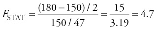
iii.The F-critical value, F_c, can be found from any F-distribution table. For example, if α = 0.05 is F_c = F_{(0.95, 2, 47)} ≈ 3.195

In Excel, to obtain F_c type = FINV(α, J, N − K) and then press Enter.

For example, type = FINV(0.05, 2, 47) then press Enter, this will give 3.195.

iv.Decision: Since F_STAT > F_c, we reject the null, meaning the two coefficients are jointly significant and implying that we should include FED in the regression.

Testing the Model Significance

To this point, Arti raises her hand and asks, “What if all coefficients of the explanatory variables in a model are zero? Cita also asks, “Does that mean that the model does not predict anything?” Dr. Theo praises them for raising the issue and says that in this case the model should be revised. Thus, the four-step procedure for the test is as follows:

i.H₀: All a_k are zeros for k = 2, 3,…, K; H_a: at least one a_k ≠ 0.

For example, in Equation 6.12, we can state that

H₀: a₂ = a₃ = a₄ = 0; H_a: at least one a_k ≠ 0.

ii.The F-statistic:

J is the number of restrictions. In the test for model significance, only a₁ is not included in the null hypothesis, so J = K − 1, and in the preceding example, J = 4 − 1 = 3.

iii.F-critical: This step is similar to the test for the joint significance.

iv.Decision: If F_STAT > F_c, we reject the null hypothesis, meaning at least one a_k ≠ 0 and implying that the model is significant.

Fligh then asks, “Can anyone analyze the relationship between t-tests and F-tests?” Mo volunteers to address the issue. Here is his discussion.

F-tests and t-tests are both testing for the significance or the expected values of the estimated coefficients. The comparison and contrast of F-test to t-test are as follows:

1.In F-test we have joint hypotheses.

2.For the test with a_k ≠ 0, the t-test is a two-tail test whereas the F-test is a one-tail test.

3.F distribution has J numerator df and (N − K) denominator df.

4.When J =1, the t- and F-tests are equivalent.

Dr. Theo is very pleased saying that all four points are correct and that we can now move to the next section.

Error Diagnostics

Heteroskedasticity and Autocorrelation

The testing procedures on these two problems in multiple linear regressions are similar to those in simple linear regressions except that the hypotheses are stated for multiple coefficients.

Testing Heteroskedasticity

Estimate the original equation

Obtain and generate then estimate the variance function:

Obtain R² for the LM_STAT = N * R ²

Using the same four-step procedure for any test, state the hypotheses as:

H₀: c₂ = c₃ = … = c_k = 0; H_a: at least one c is not zero

The next three steps are similar to the one for simple regressions with df = K − 1

Testing Autocorrelation

Estimate equation

Obtain and generate

Estimate the equation

Obtain R² for the LM_STAT = T * R ²

The hypotheses are stated as

H₀: r₁ = r₂ = … = r_k = 0; H_a: at least one r ≠ 0

The next three steps are similar to the one for simple regressions, where df = the number of restrictions.

Testing Endogeneity

Dr. Theo says that endogeneity is also called the problem of endogenous regressors and occurs when assumption (v), which states that x is not random, is violated. Given the equation

Suppose that x_i2 is random then x_i2 might be correlated with the error term. In this case the model has an endogeneity problem. The consequences of the endogeneity are serious:

i.OLS estimators are biased in small samples and do not converge to the true values even in a very large sample (the estimators are inconsistent).

ii.The standard errors are inflated, so t-tests and F-tests are invalid.

To detect endogeneity, a Hausman test must be performed. Dr. Theo says that the original Hausman test requires knowledge of matrix algebra, so he teaches us the modified Hausman test, which is discussed in Kennedy (2008).

The theoretical justification of the modified Hausman test is simple. In Equation 6.17, the exogenous variables are x_js, where When the endogenous variable x_i2 is regressed on these x_js, the part of x_i2, which is explained by x_js, will be factored out. The rest of x_i2 is explained by the residual, v_i, from the estimation:

The v_i from Equation 6.18 can be added to Equation 6.17 in the subsequent regression:

A t-test on the estimated coefficient of v_i is then performed. If this coefficient is not statistically different from zero, then x_i is not correlated with the error term, and the model does not have an endogeneity problem. Hence, the steps to perform the test are as follows:

i.Regress x_i2 on all x_js and obtain the residuals .

ii.Include the residuals in the subsequent regression of Equation 6.17.

iii.Perform the t-test on the coefficient of with the hypotheses:H₀: c = 0; H_a: c ≠ 0.

iv.If c ≠ 0, then the null hypothesis is rejected, meaning x_i is correlated with the error and implying that the model has an endogeneity problem.

Dr. Theo then asks the class, “Suppose adding into Equation 6.19 for the second regression yields = 2.5 with its standard error se () = 2.5, and N = 32. Can you find the t-statistic and make your decision?” We are able to calculate t_STAT = 2.5/2.5 = 1. Thus, c is not statistically different from zero, and we do not reject the null, meaning that x₂ is not correlated with the error and implying that the model does not have an endogeneity problem.

Adjustments

Heteroskedasticity and Autocorrelation

We learn that adjustments for these two problems are similar to the cases of simple linear regressions except that the procedures are performed on multiple explanatory variables.

Forecasting with Endogeneity

Dr. Theo then says that endogeneity problems are corrected by using the method of moments (MM). Theoretically, the purpose of the MM estimation is to find a variable w to use as a substitute for x. Theoretically, MM estimators will satisfy the condition that cov(w, e) = 0. Empirically, w almost satisfies this condition by minimizing cov(w, e), and w is called the instrument variable (IV). The MM estimators are the IV estimators. In the following section, we continue to assume that x_i2 is the endogenous variable.

The instrumental variable w has to satisfy two conditions:

i.w is not correlated with e, so that cov(w, e) = 0.

ii.w is strongly (or at least not weakly) correlated with x_i2.

In the first stage, we perform a regression of the endogenous variable x_i2 on all exogenous variables, including the IV, which is w_i:

We then estimate the original equation with the predicted value of x_i2, i2, in place of x_i2. Because of this second stage, the IV estimators are also called two stages least squares (2SLS) estimators:

The problem is solved because i2 does not contain v_i, , hence _i does not contain v either, .

Other Measures

Goodness of Fit

Although an R² value is still reported by Excel, using more than one variable decreases df. Hence, an adjusted R² value is a better measure to account for the decreasing df:

Model Specification

Dr. Theo reminds us that multiple regression models have more than one explanatory variable, so the issue of how many variables should be included in the model becomes important.

An omitted variable causes significant bias of the estimated coefficients. For example, if we remove FED from Equation 6.12 reasoning that FED is not statistically significant, then the estimated coefficients will be biased because FED and LOCAID are jointly significant. Hence eliminating FED will cause an omitted variable.

Including irrelevant variables will not significantly bias the estimated coefficients, but may inflate the variances of your coefficient estimates, so the tests are less reliable. For example, adding social assistance (SOCIAL) to Equation 6.12 will yield these results:

where the standard error of the coefficient estimate for INCOME is greatly inflated. In this case, the t-test result implies that the coefficient of INCOME is not statistically significant whereas it actually would be significant had we removed SOCIAL from Equation 6.12.

We now see that choosing a correct model is crucial. Dr. Theo says that we might want to use a piecewise-downward approach starting from all theoretically possible variables with all available data. F- and t-tests then are used to eliminate the highly insignificant variables. He says that we can also use a piecewise-upward approach, which starts from a single explanatory variable. However, the downward approach is preferable because this approach avoids the omitted variable problem that might arise if you use the piecewise-upward approach.

Excel Applications

Dr. App reminds us that the F-tests can be performed using a handheld calculator except for the critical value, the command of which has already been given in the section “F-Tests.” Also, Excel applications for the heteroskedasticity and autocorrelation tests have been given in Chapter 5. Hence, she only discusses Excel applications for the endogeneity test and correction.

Data on sale values (SALE_t), advertisement expenditures (ADS_t), income (INC_t), and values of sale coupons (COUP_t−1) are from the file Ch06.xls, Fig. 6.4 and Fig. 6.5. The model is as follows:

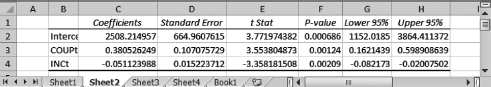
Figure 6.4 Qualification of COUP_t−1 as an instrument variable

However, we suspect that ADS_t is endogenous and so we prefer using COUP_t−1 as an IV for ADS_t. Since COUP_t−1 is in period (t − 1), it is not correlated to e_t. Since most companies include sale coupons with their advertisements and calculate the coupon values before sending out advertisements, COUP_t−1 is correlated with ADS_t. This makes COUP_t−1 a good IV for ADS_t. To perform the modified Hausman test for endogeneity, we first regress ADS on COUP and INC:

Go to Data then Data Analysis, select Regression and click OK

The input Y range is E1:E35, the input X range is C1:D35

Check the Labels box

Check the button Output Range and enter J1 then click OK

A dialogue box will appear, click OK to overwrite the data

The results are displayed in Figure 6.4.

The results support our argument that COUP_t−1 is correlated with ADS_t because the estimated coefficient of COUP_t−1 has the p-value = 0.00124 < 0.05. Additionally, by the classic assumptions, COUP_t−1 is not correlated to e_t. Therefore, COUP_t−1 satisfies both conditions to be a good IV.

Next, copy the Residuals from cells L25 through L59 and paste into cells F1 through F35

Finally, perform the regression of the original equation with the Residuals (t) added:

Go to Data then Data Analysis, select Regression and click OK

The input Y range is B1:B35, the input X range is D1:F35

Check the Labels box

Check the button Output Range and enter N22

Click OK and then OK again to overwrite the data

The main results displayed in Figure 6.5, reveal that the estimated coefficient of t, called Residuals, is significant with a p-value of 0.02 (you can find this value in cell R41 in the Excel file), so the endogeneity problem exists.

Figure 6.5 Modified Hausman test results

To correct this endogeneity problem:

Copy and paste Predicted ADS from cells K25 through K59 into cells G1 through G35

Second, copy INC in column D and paste INC into column H next to Predicted ADS

Finally regress the original equation with Predicted ADS in place of ADS:

Go to Data then Data Analysis, select Regression then click OK

The input Y range is B1:B35, the input X range is G1:H35

Check the box Labels

Check the button Output Range and enter A37

Click OK and then OK again to overwrite the data

This will correct the endogeneity problem. F-tests should be performed on the joint significance and the model significance before point and interval forecasts can be calculated.

Forecasts with Panel Data

Concept

Dr. Theo reminds us that panel data comprise cross-sectional identities over time and advises us to carry out forecasts using these data whenever they are available. Arti asks, “What do we gain from using panel data?” Alte volunteers to explain. Here is her discussion, “First, the sample size is enlarged. For example, if we have a time series dataset on TV sales in Vietnam for 16 months and another dataset on TV sales in Cambodia for the same 16 months, then combining the two datasets gives us 32 observations. Second, being able to observe more than one identity over time provides us with additional information on the characteristics of the market. For example, we can understand demand for TV in Indochina by studying their sales in Cambodia and Vietnam. Finally, we are able to carry out comparative study over time. For example, we can compare demand in Vietnam with demand in Cambodia and develop different strategies to increase sales in each country.”

Dr. Theo commends her on a good analysis and says that performing forecasts on a panel dataset is simple if the two identities share the same behavior, for example, if sales in Vietnam and Cambodia share the same market characteristics, then the coefficient estimates will be the same for the two countries. In that case, we only have to stack one dataset above the other as shown in Figure 1.1, columns G through I, of Chapter 1, and perform an OLS estimation called pooled OLS to enjoy a dataset of 32 observations.

Most of the time, the two markets do not share the same behavior. In this case, the classic OLS estimators using all 32 observations are biased, and the diagnostic tests are invalid. Hence, panel-data techniques are needed. One way to write the forecast equation is:

Dr. Theo reminds us to note the subscript “i” in a_1i indicates different intercepts across the identities. For example, Vietnam is different from Cambodia. Another way to write the relations is to also allow differences in the slopes.

Forecasting with Fixed Effect Estimators

Dr. Theo then introduces us to a way to solve the problem by using the “fixed effect” estimators. For introductory purposes, he discusses the difference in intercepts first. Theoretically, the adjustment is made by taking the deviation from the mean, so we first take an average of Equation 6.24:

Next, we subtract Equation 6.25 from Equation 6.24:

Then we can perform forecasts on the transformed model using OLS:

where

The fixed-effect problem is solved because the intercept is removed from Equation 6.26.

Empirically, the most convenient and flexible way to perform forecasts on a fixed-effect model is to use the least squares dummy variable (LSDV) approach whenever the number of identities is not too large (less than 100 identities are manageable). To obtain the LSDV estimators, we generate a dummy variable for each of the identities. For example, if we have eight different identities, then

Then Equation 6.24 can be adjusted as:

Dr. Theo reminds us that the constant is removed, so the regression does not have a constant.

We then go back to the example of the TV sales in Vietnam and Cambodia, we need to add two dummies: D_V = Vietnam and D_C = Cambodia. Thus, Equation 6.23 can be written as:

Ex asks, “What if the two markets might also differ over time?” Dr. Theo says, “Then adding time dummies to the equation will solve the problem:”

Fin asks, “How about the differences in the slopes of the two markets.” Alte suggests, “Then we can add the slope dummies to the equation:”

Dr. Theo praises her for the correct answer. He then says that point and interval forecasts can be obtained in the same manner as those in the section on “Forecasts” of this chapter.

Dr. Theo also tells us that three other approaches to correct for the problem of different characteristics in panel data are first differencing, random effect, and seemingly unrelated estimations. The first differencing approach is similar to the one used in time series analysis for AR(1) models, which will be discussed in Chapter 7. The other two methods are beyond the scope of this book. He encourages us to read an econometric book if we are interested in learning more techniques on panel data.

Detecting Different Characteristics

We want to test if the equations for Vietnam and Cambodia have identical coefficients so that OLS can be performed. This is a modified F-test for which the restricted model is:

The unrestricted model needs only one dummy because a₁₁ already catches one country’s effect:

If the two countries share the same trait, then a₁₂ = 0, so the hypotheses are stated as:

H₀: a₁₂ = 0; H_a: a₁₂ ≠ 0.

Under assumptions of equal error variances and no error correlation, this F-test is similar to the F-tests discussed in the section on “Evaluations and Adjustments” of this chapter:

where NT = the number of observations.

Dr. Theo reminds us that if we reject H₀, then the two equations do not have identical coefficients, and a panel-data technique is needed for estimations and forecasts.

Excel Applications

Ex shares with us a yearly dataset on per capita income and imports for Australia, China, and South Korea from the years 2004 to 2012 from the World Bank website. Since one lagged variable is generated, we have data for the years 2005–2012 to perform the regressions and tests. We find that the data are from the file Ch06.xls, Fig. 6.6.

Figure 6.6 ANOVA sections of the results for the restricted and unrestricted models

Testing Different Characteristics

The restricted model is:

where IMPS is imports, and PERCA is per capita income.

The unrestricted model is:

D_A and D_C are the dummies for Australia and China, respectively.

To perform the cross-equation test on the three countries, we first estimate the restricted model by regressing IMPS on PERCA:

Go to Data then Data Analysis, select Regression and click OK

The input Y range is E1:E25, the input X range is G1:G25

Check the box Labels

Check the button Output Range and enter L1

Click OK and then OK again to overwrite the data

Second, we regress IMPS on PERCA, D_A and D_C:

Go to Data then Data Analysis, select Regression and click OK

The input Y range is E1:E25, the input X range is G1:I25

Check the box Labels

Check the button Output Range and enter L20

Click OK then OK again to overwrite the data

The ANOVA sections with the sums of the squared errors for the two models are displayed in Figure 6.6: SEE_R in cell Q5 and SSE_U in cell V5 (in the Excel file, they are in cells N13 and N32, respectively).

From the results in Figure 6.6, the four steps for the test are as follows:

i.H₀: a_1A = a_1C = 0; H_a: a_1A ≠ 0, or a_1C ≠ 0, or both ≠ 0.

ii..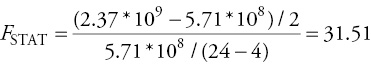

iii.We decide to use α = 0.05. Typing = FINV (0.05, 2, 20) into any cell in Excel gives us F_c = 3.49.

iv.F-statistic is greater than F-critical, so we reject the null, meaning at least one pair of coefficients is different and implying that a panel-data technique is needed.

Forecasting with Panel Data

We find that the data are from the file Ch06.xls, Fig. 6.7. We are going to perform an LSDV estimation, so the regression equation is:

Figure 6.7 Main regression results for Equation 6.28

We learn to perform the following steps:

Go to Data then Data Analysis, select Regression and click OK

The input Y range is E1:E25, the input X range is G1:J25

Check the boxes Labels and Constant is Zero, and check the Residuals button

Check the button Output Range and enter L1

Click OK and then OK again to overwrite the data

The main results are reported in Figure 6.7.

Note that the three dummies are employed to control for the fixed effects. To recover the intercept for predictions and forecasts, recall the theoretical equation:

Once the intercept is recovered, substitute it into the estimated equation to calculate the point and interval forecasts as usual. We also learn that more issues and solutions using panel data are discussed in Baltagi (2006).

Exercises

1.The file RGDP.xls contains data on RGDP, CONS, INV, and EXPS. The data are for the United States from the first quarter in 2006 to the first quarter in 2014. Given RGDP as the dependent variable:

a.Perform a correlation analysis for the three explanatory variables.

b.Perform a multiple regression of RGDP on the other three variables. Provide comments on the results, including the significances of a₁, a₂, and a₃, R², adjusted R², and the standard error of regression.

2.Write the estimated equation for the regression results for Exercise 1, enter the standard errors below the estimated coefficients, adding the adjusted R² next to the equation. Obtain the point forecast for the second quarter of the year 2014 based on this equation using a handheld calculator.

3.Use the results in Exercise 1 and carry out an additional regression on a restricted model as needed to test the joint significance of INV and EXPS at a 5 percent significance level. Write the procedure in four standard steps similar to those in the section “Evaluations and Adjustments” of this chapter. The calculations of the F-statistics might be performed using a handheld calculator or Excel.

4.The file Exps.xls contains data on EXPS, the EXCHA, and RGDP. The data are for the United States from the first quarter in 2006 to the first quarter in 2014. Given EXPS as the dependent variable:

a.Perform a multiple regression of EXPS on the other two variables.

b.Construct a 99 percent confidence interval for the one-period forecast (for Quarter 2, 2014).

c.Obtain point forecasts for two periods by applying the MA(3) for explanatory variables using either a handheld calculator or Excel.

5.The file Growth.xls contains data on GDP growth (GROW), INV, and money growth (MONEY) for four regions A, B, C, and D, in 10 years. Assuming that the four regions differ in intercepts only:

a.Perform a regression of GROW on INV and MONEY using the LSDV technique.

b.Provide point and interval forecasts for two periods ahead (m = 2).