
CHAPTER 9
Economic Models
Cita has just returned from an important meeting with the city council. The city recently established an Economic Competitiveness Office with Cita as the chair. The office is in charge of helping the private firms in three regards: (1) determining their production allocations based on the profit maximization or cost minimization principle subject to uncertainty in resources and demands, (2) calculating the changes in their input and final-good demands due to changes in technologies, and (3) making decisions on their rental prices of land to guarantee a competitive market for city land use. Cita is worried because her knowledge of economic theories is only at undergraduate level. Dr. Theo assures her that several models based on economic theories will be discussed this week. Once we finish with the chapter, we will be able to:
1.Explain the product allocation model based on economic principles.
2.Analyze changes in input and final-consumption demands of a product.
3.Develop a model for a private firm on land-use forecasts.
4.Calculate trip-distribution forecasts for the city.
5.Apply Excel while analyzing the topics in (1), (2), (3), and (4).
Most of us do not know much about economic theories, so we all look forward to gaining new knowledge.
Production Forecasts
We learn that the two production models are production allocations and input–output models. The production–allocation model helps firms forecast how much of each good to produce in the near future subject to uncertainty in the resources. The input–output model has many applications. In this chapter, it is used to forecast what will happen to the total input demand for a good if one of the technical coefficients changes and what will be the changes in the demand for final consumption of a good if one of the inputs changes.
Production Allocations
Given its historical data and interval forecasts on labor, capital, and market demand, a firm needs to forecast how much of each good it should produce the next period so that it can order inputs for its production and make a delivery plan of its production to markets. The firm is operating based on the profit maximization or cost minimization principle.
We learn that the model was first introduced by Leonid Kantorovich (1940), a Soviet mathematician and economist, during World War II to plan military expenditures based on the cost minimization principle.
The classical model for production allocations comprises three parts:
1.A linear function to be maximized (such as profits) or minimized (such as costs)
2.A set of constraints such as labor, capital, land, natural resources, and so on
3.A set of production limits that depend on market demand or quotas
The only difference between the preceding model and a forecast model for production allocations is that the forecast model faces uncertainty in resources or demand or both. Hence, this allocation forecast problem can be solved using linear programing, also called linear optimization. At this point, Dr. Theo asks our class to share our experiences if we have any. Mo says that his cousins run a factory in Europe. He puts forth a problem regarding the factory and shows us how it can be solved using a handheld calculator before using Excel.
The Ammonia Division of his cousins’ fertilizer company in Europe produces ammonium sulfate (SU) and ammonium salts (SA). Their historical data reveal that the profit rates of the two products are different:

Their production time is also different:

Additionally, the maximum limits of weekly production quantities depend on the quotas set by the provincial authority, which faces uncertainty on the quota for SA:

Another uncertainty is that there might be 120 to 150 worker hours available for the Ammonia Division four weeks from this week. Given this information, their task is to forecast how many tons of each product they should produce four weeks from now to maximize the division’s total profit.
Dr. Theo is quite pleased and tells us to work on the problem. He also decides to call the quantities of ammonium sulfate X tons and that of ammonium salts Z tons for easy applications in Excel later. Based on Equations 9.1 through 9.3, he instructs us to perform the following steps:
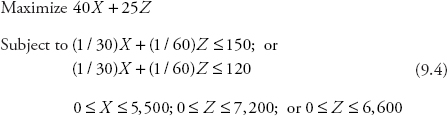
1.The linear function: Since the profits per unit are €40 for ammonium sulfate (X) and €25 for ammonium salts (Z), we are able to write the linear function for the profit maximization as:
Maximize ![]()
2.The constraints: Because 120 to 150 worker hours are available, we need to write an equation for the total worker hours, which equal the hours to make a unit of each product times quantities. We then change minutes to hours and write the constraint as follows:

Dr. Theo tells us that the constraints can be written as ![]()
![]() . Here they are written separately for Excel Solver in the next section on “Excel Application”.
. Here they are written separately for Excel Solver in the next section on “Excel Application”.
3.Production limits: We combine the aforementioned maximum limits set by the provincial authority and the nonnegative conditions for the quantities:

In sum, the problem is:
Using a handheld calculator, we first calculate the profit per hour for SU (ΠSU) and SA (ΠSA). From the constraint, one unit of SU (X) is produced in 1/30 hours whereas one unit of SA (Z) is produced in 1/60 hours, so profit per hour for each product is:

Hence, SA is more profitable to produce than SU, and Mo’s cousins want to produce up to its maximum limit of 7,200 units, which require 120 worker hours (= 7,200/60), or a maximum of 6,600 units, which requires 110 worker hours (= 6,600/60).
If they have 150 worker hours, then the remaining 30 to 40 worker hours is for SU, which will come off at 900 to 1,200 units (= 30 tons per hour * 30 hours, or = 30 tons per hour * 40 hours). If they have 120 worker hours, then the remaining 0 to10 hours is for SU, which will come off at 0 to 300 units. In brief, their forecasts for four weeks from now are:
Ammonium salts: between 6,600 and 7,200 units
Ammonium sulfate:
With 150 worker hours: between 900 and 1,200 units
With 120 worker hours: between 0 and 300 units
“Wow, that is a long problem,” we exclaim. Dr. Theo says that if we have many constraints, it will be complicated to solve by hand, so Excel is very convenient.
Input–Output Demands
Dr. Theo says there is another production forecast model based on input–output demand. Although the idea of linking various input sectors to final output sectors goes back to the 19th century, Leontief (1986) introduced the modern version that has been used widely at the present time. The model is realistic because each sector in the economy produces goods that are used as both inputs and final demands. For example, the agriculture sector provides apples and oranges as final goods for the consumers, but also as inputs for the manufacturing sector to produce apple and orange juices.
Given an economy with n sectors, each sector produces a good i that can be used as inputs for several sectors in addition to being used as a final good. Let xij be the quantity of output of good i used by sector j and xj the product of sector j; then the technical coefficient for good j is defined as:
![]()
Let y be the input demands for j = 1, 2, … n sectors. If the economy can produce m inputs, then:

If Ai is the collection of all aij used as inputs for the n sectors and Fi the final consumption of good i, then the total output of good i is:
![]()
The input–output model has numerous applications. Dr. Theo tells us that we only address a simple problem of two goods that do not require the knowledge of matrix operations. He encourages the students who are interested in a full input–output model to take a course on the general equilibrium computational model. For the problem of two goods, the equations are
![]()
![]() for i = 1 and 2
for i = 1 and 2
Cita has carried out research on the subject and shares an example on two sectors in the American economy with the class. The dataset for the output of the two sectors, agriculture (A) and manufacturing (M), is from the Bureau of Economic Analysis website:
Total output (billions of dollars)
Agriculture:XA = 420
Manufacturing: XM = 5,419
Their estimated technical coefficients are reported as follows:
| Output 1: Agriculture (A) | Output 2: Manufacturing (M) | |
| Input 1: Agriculture (A) | 0.11 | 0.05 |
| Input 2: Manufacturing (M) | 0.22 | 0.27 |
We first calculate the total input demand for each sector:
yA = AAXA = 0.11 * 420 + 0.05 * 5,419
= 46.2 + 270.95 = 317.15 ($ billions) = input demand for A.
yM = AMXM = 0.22 * 420 + 0.27 * 5,419
= 92.4 + 1463.13 = 1555.53 ($ billions) = input demand for M.
We also calculate the original demand for final consumption of the agricultural product:
![]() = 420 − 317.15 = 102.85 ($ billions)
= 420 − 317.15 = 102.85 ($ billions)
Dr. Theo then asks us to recalculate the total input demand and the demand for final consumption of the agricultural product if the technical coefficient for the agricultural product used in the manufacturing sector falls 10 percent, that is, from 100 percent to 90 percent.
We recalculate the new total input demand for the agricultural product:
yA′ = 0.11 * 420 + 0.05 * (0.90) * 5419
= 46.2 + 243.86 = 290.06 ($ billions)
We are also able to recalculate the new demand for the final consumption of the agricultural product:
![]() = 420 − 290.06 = 129.94 ($ billions)
= 420 − 290.06 = 129.94 ($ billions)
Thus, the change in final consumption of the agricultural product is 27.09 billion dollars (= 129.94 − 102.85).
Excel Application
Dr. App tells us that the exercise in the section on “Input–Output Demands” can be repeated using Excel mathematical operations. However, they are simple enough to solve using a handheld calculator. Regarding large matrices of input–output, we will need special software and so they are beyond the scope of this book. Hence, this section only uses Excel to solve the same problem in the section on “Production Allocations.” We can add as many constraints as we wish to solve without too much trouble compared to solving by hand. First, we need to install another “Add-Ins” tool.
For Microsoft Office (MO) 1997–2003:
Go to Data Tools, click on Add-Ins from the drop down menu
Click on Solve Add-in option from the new drop down menu and click OK
Whenever you need this tool, click on Data Tools and then click on Solver
For MO 2007:
Click on the Office logo at the top left that you have to click on to open any file
Click on Excel Options at the bottom center
Click on Add-Ins from the menu at the bottom of the left column in the Excel Options window
The View and Manage Microsoft Office Add-Ins window will appear
In this window, click on Go at the bottom center
A new dialog box will appear, check the Solve Ad-in box and then click OK
Whenever you need this tool, click on Data and then Solver on the Ribbon
For MO 2010:
Click on File and then Options at the bottom left column
Click on Add-Ins from the menu at the bottom of the left column in the Excel Options window
The View and Manage Microsoft Office Add-Ins window will appear
In this window, click on Go at the bottom center
A new dialog box will appear, check the Solve Ad-in box and then click OK
Whenever you need this tool, click on Data and then Solver on the Ribbon
Figure 9.1 displays the Excel spreadsheet, which is available in the file Ch09.xls, Fig. 9.1. We learn that we must proceed as follows:
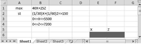
Figure 9.1 The problem and solution space in Excel
Go through cells A1 through B4 to make sure that all mathematical expressions from System 9.4 are there.
(Note that max stands for maximize, and st stands for subject to)
Highlight the solution space in cells E6 and F6 (where Solver will report the solutions).
We then open the file Ch09.xls, Fig. 9.2, because we need to enter the linear function into Excel. We find that Figure 9.2 shows what the Excel page looks like and what we should do:

Figure 9.2 Entering the linear function and the constraints
In cell A5 type Max (Maximize)
In cell A6 type = 40 * E6 + 25 * F6 and press Enter
Dr. App tells us to ignore what we see on the Excel spreadsheet temporarily because we have not opened the Solver tool). Here are the next steps:
In cell A7 type st (subject to)
In Cell A8, type = (1/30) * E6 + (1/60) * F6 and press Enter
In Cell B8, type <= and press Enter; in Cell C8, type 150 and press Enter
In Cell A9, type = E6 and press Enter
In Cell B9, type <= and press Enter; in Cell C9 type 5500 then press Enter
In Cell A10, type = F6 and press Enter
In Cell B10, type <= and press Enter; in Cell C10, type 7200 and press Enter
Do not worry about the nonnegative condition and the zero values on the page; Excel will automatically adjust the condition and the values later.
Next, we are going to open the Solver
Click on Data on the Ribbon and then click on Solver
Figure 9.3 displays the Solver Parameters dialog box and the selected parameters.
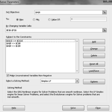
Figure 9.3 The solver parameters in the solver dialog box
In the box Set Objective enter A6
Check the button Max if it has not been checked
In the box By Changing Variable Cells enter E6:F6
Click on the box Subject to the Constraints and then click on Add
The Add Constraint dialog box will appear
Figure 9.4 displays this dialog box and the selected constraints.

Figure 9.4 The add constraint dialog box with the first constraint entered
In the box Cell Reference enter A8
Click on the arrow of the next box to choose <=; in the box Constraint enter C8
Once you finish entering this constraint, click Add to add the next two constraints
In the box Cell Reference enter A9
Click on the arrow of the next box to choose <=
In the box Constraint enter C9 and click Add
In the box Cell Reference enter A10
Click on the arrow of the next box to choose <=; in the box Constraint enter C10
After the last constraint is entered, click OK to return to the Solver shown in Figure 9.3
Use the arrow in the Select a Solving Method box to choose Simplex LP (linear program)
Click on Solve at the bottom right next to Close; a new dialog box will appear
Select Keep Solver Solution and click OK
We now see the quantity 900 and 7200 appearing in cells E6 and F6 in Figure 9.5 or in the file Ch09.xls, Fig. 9.5.

Figure 9.5 The first production allocation for ammonium division
We learn that we should repeat the same procedures for the other constraints of the 120 worker hours and production limit of 6,600 units.
Gravity Models
We are delighted to learn that we are going to modify a model that is based on Newton’s law of gravitational attraction:
![]()
| where f1, 2 = | the gravitational attraction force between any two objects |
| m1 = | the mass of the first object |
| m2 = | the mass of the second object |
| d1, 2 = | is the distance between the two |
The parameter k is a measure of gravitational attraction and has to be decided case by case based on the characteristics of the masses. For example, if the gravitational attraction between the two is one half of their masses, then the parameter k = 0.5.
Gravity models have many applications. In econometrics, it is used to predict bilateral trade between two countries, which depends positively on their income and negatively on their distance in addition to several other determinants. Dr. Theo says that we only discuss two cases in forecasting: land use and trip distribution. He also reminds Cita that the land-use model is closely related to her job at the Economic Competitiveness Office.
Land-Use Forecasts
We learn that the early studies on land distribution focused on the population density in the cities and found that urban population is crowded around the downtown area and gradually spread out in the more remote areas. However, in this class, we focus on a model introduced by Dunn (1954) for land-use forecasting in both urban and rural areas. This model is simple but has useful applications and is related to the gravity model in that one of the factors that affect the land use (called determinants of the land use) is the distance to the market:
![]()
where
| Rt+1 = | the rental price per unit of land at time (t + 1) |
| Q t = | the quantity of production at time t |
| Pt = | the market price per unit of production at time t |
| Ct = | the production cost per unit of production at time t |
| Tt = | the unit transportation cost at time t |
| d = | the distance from the firm’s headquarter to the market |
From this equation, the first group on the right-hand side is the profit from the production process, that is, QP is total revenue and QC the total cost. The second group on the right-hand side is the cost of transportation to the market for any firm. Hence, the right-hand side is the net profit of the firm, and the breakeven point is where the rental price per unit of land equals the net profit of the firm. Data on Q, P, C, T, and d are collected for the current period, and the forecast of the rental price for the next period is calculated.
At this point, Fligh says that he can offer an example from his friend, who is the manager of a firm that produces tractors in the city. His firm produces 100 tractors per month that can be sold for $100,000 each. The cost to produce a tractor is $60,000. The transportation cost is $100 per mile per tractor and the distance to the tractor dealer is 100 miles.
Dr. Theo is very pleased and asks us to substitute these data into Equation 9.8 to forecast his rental price next month.
![]()
Hence, his rental price for the next month should be roughly $3,000,000 in order to break even and survive the competition from other companies.
Trip-Distribution Forecasts
We learn that the trip distribution model is popular in transportation forecasts. The model was initially used to understand how people accept a job offer or remain in a job, and lately it has been used to predict the pattern of transportation between two regions, often called the origin and destination. We start with a simple version of the Voorhees (1956) model for trip-distribution forecasting with one origin where workers (W) live and one destination where the jobs (J) are offered. In this case, the forecast model is:
![]()
The parameters a, b, c are friction factors that have to be calibrated based on actual surveys, for example, a is the friction factor for the workers and shows the reluctance of the people who make the trips to a job based on their family conditions at home, b is the friction factor for the jobs and reveals how attractive a job is, and c is the friction factor for the travel costs and indicates how much people are willing to travel to various distances. The calibration of the trip-distribution model involves adjustments of these friction factors.
Given this model, we want to forecast how many round trips the workers will make from their hometown to their workplaces. Levinson and Kumar (1994, 1995) suggest several models for friction factors; the most commonly used model is:
![]()
If a survey found that the most significant cost between two regions is the distance, and the relation is
![]()
then substituting Equations 9.10 and 9.11 into Equation 9.9 will allow us to calculate TOD:
![]()
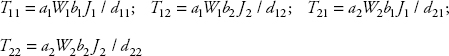
Dr. Theo then extends the original model for two regions to a model for four regions. The friction factors can now be written as:
The number of round trips between two regions is then calculated using these equations:

Arti raises her hand and says her friend works for the county office and has a problem that needs to be solved. The four regions in her province are: Ami (A), Bero (B), Cira (C), and Dore (D). Data for the number of workers (W), the number of jobs (J), and the distances (d) between them are provided in Table 9.1.
Table 9.1 Workers/jobs and distance among four regions
| Workers/jobs (in thousands) | W (in miles) | J | Distance dij | 1 (A) | 2 (B) |
| 1 (C) | 30 | 40 (A) | 1 (C) | 24 | 18 |
| 2 (D) | 35 | 32 (B) | 2 (D) | 28 | 25 |
A survey of the friction factors between any two regions in her provinces yields the following equations:
![]()
![]()
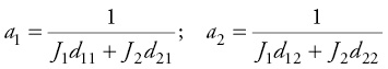
We are more than glad to help Arti’s friend find the solutions. The calculations can be done using a handheld calculator and then Excel. First, we use this information to calculate the friction factors:
a1 = 1/(40/24 + 32/28) = 1/(1.67 + 1.14) = 1/2.81 = 0.3559
a2 = 1/(40/18 + 32/25) = 1/(2.22 + 1.28)= 1/3.5 = 0.2857
b1 = 1/(30/24 + 35/28) = 1/(1.25 + 1.25) = 1/2.5 = 0.4
b2 = 1/(30/18 +35/25) = 1/(1.67 + 1.4) = 1/3.07 = 0.3257
We then forecast the number of round trips between two regions by substituting these data into Equation 10.16:

Arti is very happy. She is going to show the solutions to her friend.
Dr. Theo reminds us that trip-distribution forecasts for more than four regions requires knowledge of matrix algebra and that a comprehensive analysis of N regions is presented in Tsekeris and Stathopoulos (2006) for our reference.
Excel Application
Dr. App tells us that the exercise in the section on “Land-Use Forecasts” is simple enough to solve using a handheld calculator. Thus, we only use an Excel spreadsheet to solve the problem in the section on “Trip-Distribution Forecasts”. Figure 9.6 displays data on the number of workers, number of jobs, and the distances.

Figure 9.6 Data and calculations of friction factors
Dr. App tells us to open the file Ch09.xls, Fig. 9.7, and enter the following commands:

Figure 9.7 Data and calculations of friction factors
In cell H1, type = 1/((C2/E2) + (C3/E3)) and press Enter
In cell H2, type = 1/((C2/F2) + (C3/F3)) and press Enter
In cell H3, type = 1/((B2/E2) + (B3/E3)) and press Enter
In cell H4, type = 1/((B2/F2) +(B3/F3)) and press Enter
Figure 9.7 displays the same data and calculations of round trips between pairs of cities. We open the file Ch09.xls, Fig. 9.8, and proceed as follows:
In cell J1, type = (H1 * H3 * B2 * C2)/E2 and press Enter
In cell J2, type = (H1 * H4 * B2 * C3)/F2 and press Enter
In cell J3, type = (H2 * H3 * B3 * C2)/E3 and press Enter
In cell J4, type = (H2 * H4 * B3 * C3)/F3 and press Enter
Dr. App asks us to compare the results using the Excel spreadsheet with those using a handheld calculator. We find that they are the same once the values on the Excel spreadsheet are rounded off to two decimal places.
Exercises
1.The Pan Division of a kitchen-appliance manufacturer produces two kinds of pans: large (L) and small (S). Their historical data reveal that the profit rates of the two products are:
| Profit per unit (dollars per pan) | L | $4.0 |
| S | $2.2 |
| Time (minutes per unit): | L | Two minutes |
| S | One minute |
From the firm’s plan, between 180 to 200 worker hours will be available for this Pan Division next week. Additionally, the maximum limits of weekly production quantities depend on the quotas set by the plant leaders:
| Maximum limits (units): | L | 6,000 |
| S | 8,400 |
Use a handheld calculator and then an Excel spreadsheet to forecast how many units of each product this Pan Division should produce next week to maximize the division’s total profit.
2.Data on two manufacturing sectors in an economy are given in the following text:
| Total output (millions of dollars) | |
| Meat processing: | XM = 250 |
| Vegetable processing: | XV = 180 |
Their estimated technical coefficients are reported as follows:
| Output 1: Meat (M) | Output 2: Vegetables (V) | |
| Input 1: Meat (M) | 0.20 | 0.10 |
| Input 2: Vegetables (V) | 0.10 | 0.05 |
a.Calculate the total input demand for each sector.
b.Calculate the original demand for final consumption in the vegetables sector.
c.Recalculate the total input demand and the demand for final consumption if the technical coefficient for the vegetable products used in the meat processing sector falls 50 percent (from 100 to 50 percent).
3.Given the trip-distribution model involving four regions—A, B, C, D—with workers and jobs in thousands and distances in miles, the equations of the friction factors are as follows:

The equations for the round trips between two regions are:
The data for the regions are provided in Table 9.2.
Table 9.2 Workers, jobs, and distances
| Workers/jobs (thousands) | W | J | Distance di (miles) | 1 (A) | 2 (B) |
| 1 (C) | 24 | 30 (A) | 1 (C) | 22 | 16 |
| 2 (D) | 26 | 34 (B) | 2 (D) | 28 | 18 |
Use a handheld calculator and then an Excel spreadsheet to calculate the friction factors and forecast the number of round trips between any two regions.