
CHAPTER 10
Business Cycles and Rates of Change
Fligh has a conversation with Dr. Theo before class. His company, Flightime Airlines, is engaged in a fierce competition with a new arrival, Skylight, which started very small but has attracted customers away from his Flightime by undercutting airfares. Currently, Flightime is still ahead of Skylight in their respective sales. However, he heard that sales at Skylight have been growing at a rate of 7.5 percent monthly whereas sales at his Flightime have only grown at a rate of 2 percent. He is worried that Skylight will soon catch up with his company’s sales and wants to find out when that will happen if their respective rates remain at 7.5 and 2 percent.
Dr. Theo tells him this issue of catching up will be one of the topics for this week. Upon completing the chapter, we will be able to:
1.Describe the concept of business cycles and economic leading indicators.
2.Construct a diffusion index for these indicators to predict the economic turning point.
3.Explain the catching-up models using the rates of change concept.
4.Develop various investment strategies.
5.Obtain forecasts for (2), (3), and (4) using Excel.
Forecasts on the turning points of the economy use business cycle measurements and rates of change. Forecasts on catching up and investment choices are based on rates of change only.
Turning Points
We have learned that a time series often has a cyclical component. The difference between any cyclical component of any time series and the business cycles is that the latter fluctuate around a long-run trend in real gross domestic product (RGDP). When the RGDP is approaching a peak, the economy is in an expansionary period. When the RGDP is approaching a trough, the economy is in a recessionary period. The technique we are going to learn helps us forecast the turning point, when the economy changes its direction. The technique can also be applied to the business forecast of a company’s turning point based on the company’s leading factors.
Theoretically, an economy is in recession (having a turning point) if its RGDP falls continuously for six consecutive months. Also, an economy is in a period of expansion if its RGDP rises continuously for six consecutive months. In reality, RGDP might go down for four months, inch up slightly in the fifth month then decline again in the next two months, making it hard to conclude whether the economy is having a turning point.
To help forecast a turning point in the economy, various measures called economic indicators are developed. The Conference Board, a global nonprofit organization for businesses, publishes the Global Business Cycle Indicators for each month on its website. The list always comprises indices of the leading, the coincident, and the lagging indicators, as well as their rates of change.
Concept
The leading indicators occur before a turning point and so provide a warning of a possible change in the direction of the economy. The coincident indicators happen concurrently with a change in the direction of the economy, and the lagging indicators measure factors that change after the economy has already followed a new pattern. Only leading indicators help with forecasting and will be discussed in this chapter. The most recent leading indicators published by the Conference Board are as follows:
Average weekly hours in the manufacturing sector
Average weekly initial claims for unemployment insurance
Manufacturers’ new orders of consumer goods and materials
Institute for Supply Management (ISM) index of new orders
Manufacturers’ new orders of nondefense capital goods
Building permits for new private housing units
Stock prices for 500 common stocks
Leading credit index
Interest rate spread for the 10-year Treasury bonds minus the federal funds target
Average consumer expectations for business conditions
Fin then tells us that some of the leading indicators affect the economy very strongly. For that reason, the business reporters, who are allowed to enter the locked rooms in Washington, DC, where the statistics are released, often write frantically in their 30-minute allowance before breaking their stories to the world. In the meantime, the tension level is also high worldwide, where corporate leaders, business managers, financial advisors, and individual investors are staring at their computer screens waiting eagerly for the news release. This is what Fin encounters on most of his weekdays.
Dr. Theo thanks him for sharing his experience and then summarizes the general opinion of several experts on the leading indicators to help us understand the concept. He says that the detailed analyses can be found in Rogers (2009), Baumohl (2008), or Ellis (2005).
Average Weekly Hours in the Manufacturing Sector
This series is a leading indicator because any adjustment to the working hours of existing employees is usually made in advance of a new hire or layoff. The indicator measures new jobs created, the unemployment rate, average hourly earnings, and the length of the average workweek. Since consumer spending rises with employment, this is a much anticipated indicator for each month and can be considered a highly sensitive series for forecasting.
Since the indicator contains information about both job and wage growth, several economists choose to focus more on the wage data than on the employment data, arguing that it is the income that drives spending instead of employment. This argument has gained attention recently due to the slow recovery period from 2009 to 2013 when employment was growing but wages remained flat.
The data are reported by the U.S. Department of Labor on the first Friday of each month at 8:30 a.m. Eastern time for the previous month.
Initial Jobless Claims
This series is reported weekly and measures the number of people filing first-time claims for state unemployment insurance. It is more sensitive than other measures of unemployment because laid-off workers usually file claims immediately either to receive unemployment benefits or to look for a new job if they are not qualified for the benefits. The series can be considered highly sensitive. However, the series is also very volatile and requires revisions by taking four-week moving averages to smooth out the volatility in claims.
The data are reported by the U.S. Department of Labor every Thursday at 8:30 a.m. Eastern time for the previous week.
Manufacturers’ New Orders of Consumer Goods and Materials
This information is considered a leading indicator because it reflects the changes in consumer demand and hence leads to changes in actual production. Its official name is the Preliminary Report on Manufacturers’ Shipments, Inventories, and Orders and is a measure of shipments (sales), inventories, and orders at the manufacturing level.
The data are reported by the U.S. Bureau of the Census during the first week of the month at 8:30 a.m. Eastern time for the previous two months. Since the data are two months old, the index is not considered a good prediction of the economy and can be considered a low sensitive series.
ISM Index of New Orders
This index is compiled by the ISM and is one of the first released each month that is believed to have a high impact on the markets. It is a leading indicator because orders of inputs have to be placed in advance of the production. The indicator is based on a survey of purchasing at roughly 300 industrial companies and is considered the best indicator for the manufacturing sector.
Surprisingly, the series does not help as much in forecasting as expected. Perhaps the index is calculated from nine subindexes: new orders, production, employment, supplier deliveries, inventories, prices, new export orders, imports, and backlog of orders. Some of these subindexes are determined only once the economy has already settled in a clear pattern instead of leading the economy. Hence, the series can be considered moderately sensitive.
The data are released by the ISM on the first business day of the month at 10 a.m. Eastern time for the previous month.
Manufacturers’ New Orders for Nondefense Capital Goods
This information is considered a leading indicator because investing in capital goods requires long-term plans, so firms do not place new orders unless they realize positive changes in actual production and rising demand.
The data are reported by the U.S. Bureau of the Census during the first week of the month at 8:30 a.m. Eastern time for the previous two months. Since the data are also two months old, the index is not considered a good prediction of the economy and can be considered a low sensitive series.
Building Permits for New Private Housing Units
This information leads the economy because a construction firm does not apply for a building permit until a contract for a new building in the near future is signed with a customer. Since construction is a large investment, it is supposed to have a large impact on the economy. Officially named Housing Starts and Building Permits, the indicator also measures the number of buildings already under construction in addition to the number of permits.
The series is a leading indicator of home sales and spending in general. However, consumers and firms usually do not invest until the economy has already shown signs of improvement from a recession. Also, in an economic expansion, building permits and new houses continue to be built until a recession looms large. Hence, the series can only be considered moderately sensitive.
The data are released by the U.S. Bureau of the Census around the 18th day of the month at 8:30 a.m. Eastern time for the previous month.
Stock Prices of 500 Common Stocks
This dataset is from the Standard & Poor’s 500 (S&P 500) and is considered a leading indicator because changes in stock prices reflect the investor’s expectations for the future of the economy. The S&P 500 incorporates the 500 largest companies in the United States and so its price change is a good measure of the movements in the stock prices. The S&P 500 stock prices are posted on The Wall Street Journal website and various other websites every weekday. So it is very timely and highly sensitive.
The index is reported in the third or fourth week of each month by the Conference Board based on the previous month’s data.
Leading Credit Index
This index is a new indicator at the Conference Board, introduced to replace the previous indicator of Money Supply, which no longer predicts the turning point of the RGDP very well but has trailed behind the economy since 2008. The credit index is constructed based on the several subindicators that predict the movements in the financial markets and can lead the economy.
The indicator was initially released on January 26, 2012, by the Conference Board for the previous month and has been reported in the third or fourth week of each month by the board since then. It has been welcomed by the professional world as a highly sensitive series.
Interest Rate Spread of the 10-Year Treasury Less Federal Funds Target
This measure is usually referred to as the term spread, which is highly sensitive because a long-term bond has to yield a higher rate than a short-term one in order to attract any investor at all due to the risks involved in holding a long-term bond. It is a leading indicator because right before a recession, the spread between the short-term and long-term bonds becomes closer. Then the yield of long-term bonds declines sharply during a recession, which causes a negative spread.
The difference between these two series can also be studied in a yield curve, which is upward-sloping over time in the normal situation with the yield of the short-term bond much smaller than that of the long-term. A change in the direction of this curve, called an inverted yield curve, can predict a recession in the economy. Recently this indicator has lost favor among the professionals because it failed to predict the 1990–91 and the 2007–08 recessions. Hence, the series can only be considered moderately sensitive.
Interest rates are posted on The Wall Street Journal website and various other websites every weekday.
Average Consumer Expectations for Business Conditions
This information is the only leading indicator that is based solely on expectations. The indicator measures consumer confidence and leads the economy because it can indicate an increase or decrease in consumer spending that affects the demand side of the economy. Unfortunately, consumer confidence changes quite often depending on daily news regarding stock markets and the world economy, so the series can be considered moderately sensitive.
The indicator is released by the University of Michigan in two rounds: The first round is on the 15th of the month (a preliminary reading), and the second round is on the last business day of the month (a final reading) at 10 a.m. Eastern time for the current month.
Constructing Diffusion Indexes
Dr. Theo reminds us that the Conference Board also calculates a composite index that averages the 10 leading indicators and adjusts for seasonal fluctuation. A simple idea is to look at this composite index. If it goes down for three consecutive months, one might predict a coming recession and vice versa.
For example, the Conference Board reported on December 22, 2014, that the Leading Economic Index for the United States increased 0.8 percent in September, followed by a 0.6 percent increase in October and a 0.6 percent increase in November. This is a consistent three-month rise and might predict an economic expansion in the near future.
At this point, Fin raises his hand and asks, “Is predicting a turning point so easy?” Dr. Theo answers, “No, actually this rule is too simple to give a reliable prediction in reality, especially in predicting a recession. Additionally, if you come from a developing country, the 10 preceding indicators might not fit your country’s conditions, and you might want to track a different set of indexes. Hence, a diffusion index for each month will take into account the rates of change in all relevant indicators and help you construct your own indexes instead of looking at the single composite index provided by the Conference Board.”
There are several approaches to calculating the diffusion indices. Dr. Theo says he has compiled the steps presented in the following text based on the suggestions of the Conference Board:
i.Calculate the rate of change for each indicator:

where I is an individual index for a leading indicator
For example, if an index changes from 20 to 19 going from January to February, then the rate of change between the two months is:

ii.Ascribe an assigned value (AV) to each change:
1 to a positive change
0.5 to the unchanged one
0 to a negative change
This raises a question of how much change should be considered a true change.
The Conference Board suggests that a positive movement is any rise that is equal to or greater than 0.5 percent, and a negative movement is any fall that is equal to or greater than 0.5 percent. This implies that any change less than 0.5 percent constitutes an unchanged variable.
iii.Sum the AV calculated in step (ii), divide the sum by the number of indexes, and multiply the ratio by 100.
We then break into groups to work on an example: Table 10.1 shows the following monthly indexes of eight leading indicators in a hypothetical economy between January and February 2013 and the steps to calculate a diffusion index for February. The results show an index of 62.5, which is above the average index of 50 and implies a stable economic condition.
Table 10.1 Calculating a diffusion index
| Indicators | 1 | 2 | 3 | 4 | 5 | 6 | 7 | 8 | Diffusion index |
| January | 20 | 30 | 15 | 40 | 28 | 14 | 30 | 40 | |
| February | 19 | 30.1 | 16 | 39 | 30 | 15 | 31 | 40 | |
| (i) %Δ | −5 | 0.3 | 6.7 | −2.5 | 7.1 | 7.1 | 3.3 | 0 | |
| (ii) AV | 0 | 0.5 | 1 | 0 | 1 | 1 | 1 | 0.5 | |
| (iii) Index: | [(0 + 0.5 + 1 + 0 + 1 + 1 + 1 + 0.5)/8] * 100 | = 62.5 | |||||||
Dr. Theo says that in his opinion, you have to continue to track the diffusion indexes for at least five months. If the diffusion indexes are below 50 for 80 percent of the time, the economy has a high probability of landing in a recession and vice versa. Additionally, if more than seven out of 10 individual indexes are falling, the economy looks gloomy. The severity of the gaps in the diffusion indices also have to be taken into account, for example, a negative gap of 20 points from the average of 50 points implies a severe condition compared with a gap of five points.
Arti then asks, “We are talking about economic recessions and expansions. But then why is the cycle called a business instead of an economic cycle?” Alte offers to answer. Here is her explanation: “The up and down cycle of the economy depends on the business activities. When businesses are growing, they start to invest in new capital, which causes the economy to expand for several years until it reaches a peak. Then businesses are no longer growing, and there is no additional capital. Gradually, the plants and capital are worn out, and the economy is approaching a trough. This cycle is renewed when depleted capital is replaced by a new one.”
“Excellent,” Dr. Theo commends her. He then continues with the discussion of the diffusion index by saying, “The Conference Board also suggests that you construct a six-month diffusion index. In this case, you list all six months first and see if an individual index is going up or down at the end of the six-month period.”
Dr. Theo believes that a six-month diffusion index is not much of a difference from the Conference Board composite index because it provides only one index for the whole six-month period. Moreover, he does not believe this diffusion index is of much help in forecasting because the economy is already in a recession after six months of continuous declining RGDP, so it is too late to predict the situation. Hence, he suggests, “If you wish to have longer-term indices, you can construct two-month or three-month indexes, which give more room to think ahead of a possible turning point.”
One remaining issue with diffusion indexes is that the Conference Board and current researchers treat them equally. Dr. Theo also believes some weighted approaches should be used to account for the difference in the level of sensitivity in the released data. He says that scrutinizing Excel applications will clarify this point.
Excel Applications
Dr. App shows us Figure 10.1, which displays the data from the file Ch10.xls, Fig. 10.2, on 10 indexes of the leading indicators for a hypothetical economy from January through July 2014.
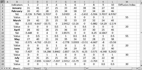
Figure 10.1 Obtaining diffusion indexes for February through July 2014
We learn that the following steps must be performed:
In cell C4, type = ((C3 − C2)/C2) * 100 and press Enter
Copy and paste the formula into cells D4 through L4
In cell C7, type = ((C6 − C3)/C3) * 100 and press Enter
Copy and paste the formula into cells D7 through L7 and into the following cells:
Cells C10 through L10
Cells C13 through L13
Cells C16 through L16
Cells C19 through L19
Enter values 0, 0.5, or 1 by looking at the percentage changes
For example, the value in cell C4 is −3.226. This implies a fall of 3.226 percent, which is more than a 0.5 percent decrease, so enter 0. Once you finish entering all values of 1, 0.5, or 0:
In cell M5, type = ((C5 + D5 + E5 + F5 + G5 + H5 + I5 + J5 + K5 + L5)/10) * 100 and press Enter
Copy and paste the formula from cell M5 into cells M8, M11, M14, M17, and M20
The diffusion indexes are in column M.
The results reveal that only four out of six indexes are below 50, which is only 67 percent below 50 instead of the 80 percent benchmark mentioned by Dr. Theo in his theoretical section. Alte asks, “Should we still send a warning that the economy is heading into a recession?” Dr. App says, “Here is my interpretation of the indexes: The two indexes above 50 are just 5 points from the 50 level, whereas the ones below 50 show gaps of 20 to 30 points. Based on this observation alone, I would rather send a warning on a high probability of a recession.”
Dr. App now comes to Dr. Theo’s last point in the section on “Constructing Diffusion Indexes”: Should we use a weighted approach to constructing diffusion indexes? Dr. App says that she also believes in a weighted-index approach. However, she warns us, “This is the technique suggested by this class’ instructors, so take it at your own risk.” Here is the idea: We can assign different weights across the leading indicators based on their own level of sensitivity, either high (H), low (L), or moderate (M). For example, Table 10.2 lists the leading indicators reported by the Conference Board, their sensitivity, and possible weights.
Table 10.2 Assigning different weights across leading indicators
| Indicator | 1 | 2 | 3 | 4 | 5 | 6 | 7 | 8 | 9 | 10 |
| Sensitivity | H | H | L | M | L | M | H | H | M | M |
| Weight | 2 | 2 | 1 | 1.5 | 1 | 1.5 | 2 | 2 | 1.5 | 1.5 |
Hence, the total of the weighted indexes are:
Total = 2 + 2 + 1 + 1.5 + 1 + 1.5 + 2 + 2 + 1.5 + 1.5 = 16
The steps of calculations are as follows:
i.Calculate the rate of changes for each indicator using Equation 10.1 as usual.
ii.Ascribe a value of 1 to a positive change, 0.5 to the unchanged one, and 0 to a negative change. After that multiply the values by 2 and 1.5 for the highly sensitive and moderately sensitive indicators, respectively.
iii.Sum the value calculated in step (ii), divide the sum by 16, and multiply the ratio by 100.
Figure 10.2 displays the data from the file Ch10.xls, Fig. 10.4, as well as the new calculations. From the results, we are now more confident to conclude that the economy is heading into a recession because all six diffusion indices are below 50 with many substantially so.
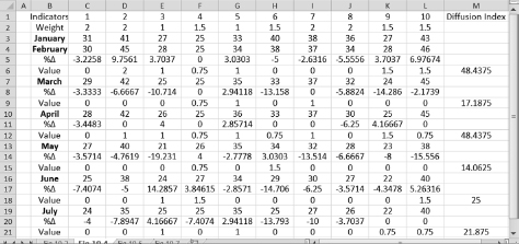
Figure 10.2. Obtaining diffusion indexes using weighted indicators
We then work with Dr. Theo on several models based on rates of change.
Models Based on Rates of Change
We learn that we can apply the rates of change concept to models in this section to forecast catching-up games and investment choices. The original ideas are from Thirlwall (2003) and are modified to fit the business problems in this section.
Catching Up
Rates of change can be used to study convergence (or catching up) among countries or companies. For example, the sales of Fligh’s company have grown at a monthly rate of 2 percent whereas those of Skylight have grown at a monthly rate of 7.5 percent. How long would it take Skylight to catch up with Flightime at their respective growth rates?
In economic theory, there is an unconditional convergence where developing countries will catch up with the developed countries even if the former do not grow faster than the latter. There are three arguments for this unconditional convergence.
First, the neoclassical growth theory assumes diminishing returns to capital. A developed country, which has accumulated a large stock of capital per worker over time, will eventually reach a long-run equilibrium called the steady state, where the country’s growth rate of capital per worker will be zero. This will allow a developing country to catch up and the two will converge to the same level of RGDP.
Second, since knowledge and technology are considered public goods, there are positive externalities flowing from developed to developing countries. These knowledge and technology transfers and spillovers allow the developing countries to harvest benefits from the developed countries without costs because the former do not have to fund the research and development (R&D) that results in new knowledge and technology.
Third, the progress from an underdeveloped economy to a developed one always goes through an industrialization process. During this process, the factors of production and resources are automatically moving from the agricultural sector with low productivity to the manufacturing and service sectors with high productivity. Since resources cannot be shifted forever, developing countries will have greater shifts of resources and be able to catch up.
Empirically, there is no clear evidence of unconditional convergence. There are certain conditions for the convergence to occur. The conditions for a country could be high investment in education, a higher savings rate, or good governance.
The following section modifies the original ideas to forecast catching points between two companies. The conditions for a company to catch up with another company could be corporate restructuring, high investment in capital, rigorous R&D funding, or simply launching an aggressive campaign.
Catching Up to Current Level
Given an average growth rate in the sales of a small company, we can find how long it would take a small company to catch up with a large company, whose sales do not grow. The relationship between the former and the latter can be expressed as:
![]()
where
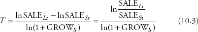
Taking the natural logarithm of Equation 10.2 yields:

Solving for T to obtain:
To this point, Fligh raises his hand and asks, “Can we apply this problem to calculate how long it would take for Skylight to catch up with Flightime if my company does not grow?” Dr. Theo replies, “Sure, let’s work on the problem.”
Fligh provides the class with the information: His company’s sales this month are $134,840, and Skylight’s sales are $45,040. We already know that monthly sale growth at Skylight is 7.5 percent, so
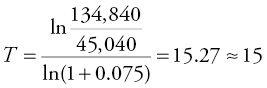
Hence, it would take Skylight roughly 15 months at a growth rate of 7.5 percent to catch up with Flightime if the latter does not grow.
Catching Up at Future Level
Dr. Theo then says, “But Flightime is also growing, so we need to revise Equation 10.2 to find how long it would take for the gap between the two companies to be eliminated in the future.” The relationship between the former and the latter can be expressed as:
![]()
where GROWL = the sale growth rate of the large company
Taking the natural logarithm of Equation 10.4 yields:

Solving for T to obtain:
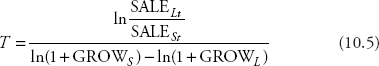
Dr. Theo then says, “Let’s work on the problem between Flightime and Skylight again.” We already know that the monthly sale growth at Fligh’s company is 2 percent, and the monthly sale growth at Skylight is 7.5 percent; hence:
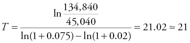
Thus, it takes Skylight roughly 21 months to catch up with Flightime’s sales. Fligh exclaims, “That is fast! I will report this result to my boss so that he can pursue an aggressive campaign to increase sales. Otherwise, we might soon go bankrupt.”
Required Growth Rate to Reach a Target
Dr. Theo continues, “In solving the problem in Equation 10.5, we assume that Skylight is growing at a constant rate of 7.5 percent. Suppose that Flightime continues to grow at a 2 percent rate, but Skylight sets a target to catch up with the Flightime in 25 months instead of 21 months. It then needs to calculate the required growth rate to reach that target.” We can start from Equation 10.4:

We work on the problem again by substituting 25 months, sales for the two airlines, and the sale growth of 2 percent for Flightime into Equation 10.6:
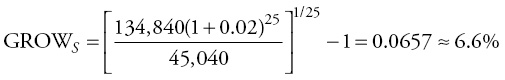
Thus, Skylight has to grow at a monthly rate of 6.6 percent to eliminate the gap in 25 months.
Required Growth Rate to Keep a Constant Gap
Dr. Theo discusses the last case of the catching-up games: Suppose Skylight is running out of resources to compete with Flightime at this moment and wants to know what growth rate will keep the gap between the two companies constant until a certain date in the future, say 25 months from now. In this case, the equation is:
![]()

We work on the airline problem a last time:

Therefore, Skylight can keep the gap at a constant value for 25 months if its sales grow at a monthly rate of 4.4 percent.
Investment Choices
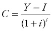
Cita shares with us a problem from the city council. The mayor wants to make decisions on various investment possibilities. He wants Cita to help with finding the right mix of strategies and time horizons to maximize the city’s welfare in the future. Cita provides us the following information:
The city economy has a capital output ratio of 1.5, that is, K/Y = 1.5, and so Y = K/1.5.
The initial capital stock is $390 million.
The depreciation rate is 10 percent (d = 0.1), so the capital for the next period = K (1 − d) unless a new investment is made.
Consumption is chosen as the measure of the city welfare.
The social discount rate is 1 percent (i = 0.01).
For starting, we assume no government spending; hence:
 ; t = 0, 1, 2, 3, 4.
The mayor is newly elected in November and has four years ahead as his time horizon. He has to make a decision between two investment scenarios: the first is to invest 8 percent of the output and have more output value for current consumption. The second is to invest 9 percent of the output and have less output value for current consumption but more for future consumption.
The mayor wants to make a decision on the plan that will maximize the city’s welfare in four years. We work on the calculations and display them in Table 10.3.
Table 10.3 Making investment decision
| Year | Plan 1 (I/Y = 8%; d = 0.1; i = 1%) | Plan 2 (I/Y = 9%; d = 0.1; i = 1%) | ||||||||
| K | K(1−d) | Y | I | C | K | K(1−d) | Y | I | C | |
| 0 | 390 | 390 | 260 | 20.8 | 239.2 | 390 | 390 | 260 | 23.4 | 236.6 |
| 1 | 410.8 | 369.72 | 246.5 | 19.7 | 224.5 | 413.4 | 372.1 | 248 | 22.3 | 223.5 |
| 2 | 430.5 | 387.5 | 258.3 | 20.7 | 233.0 | 435.7 | 392.2 | 261.4 | 23.5 | 233.2 |
| 3 | 451.2 | 406.1 | 270.7 | 21.7 | 241.7 | 459.3 | 413.3 | 275.6 | 24.8 | 243.4 |
| 4 | 472.8 | 425.6 | 283.7 | 22.7 | 250.8 | 484.1 | 435.6 | 290.4 | 26.1 | 254.0 |
The results show that the second plan yields more capital than the first one: by the end of the first year, the first plan has $410.8 million (= 390 + 20.8) whereas the second plan has $413.4 million (= 390 + 23.4). Hence, by the end of the second year, the second plan already yields a better consumption value of $233.2 million (= [261.4 − 23.5]/[1.01]2) compared with $232.9 million (= [258.3 − 20.7]/[1.01]2) for the first plan. Additionally, output and capital stock grow at faster rates with the second plan thanks to the high rate of investment, opening a venue for future growth. However, if the mayor has only one year to go, he should choose the first plan with the 8 percent investment rate because by the end of the first year, the first plan yields a better consumption value of $224.5 million compared to $223.5 million for the second one.
Dr. Theo tells us that Excel applications conducted by Dr. App will add government spending and use more time horizons.
Excel Applications
Dr. App says that the problems in the section on “Catching Up” can be solved faster with a handheld calculator, so she only shows us Excel demonstrations for the investment problems in the section on “Investment Choices.” The problem is to choose between two investment plans: the first one invests 8 percent of the output, and the second invests 16 percent of the output. The depreciation rate is 10 percent, and the discount rate is 3 percent. The capital output ratio equals 3, and government spending is fixed at $10 million. Figure 10.3 shows data from the file Ch10.xls, Fig. 10.6. Dr. App tells us to proceed with the following steps, ignoring the results in each column for a while because they will be gradually adjusted:
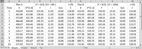
Figure 10.3 Obtaining forecasts on future consumption from two investment plans
In cell D3, type = C3/3 and press Enter
(Note that the values in cells B3, C3, H3, and I3 are initial capital with d = 0 for t = 0)
Copy and paste the formula from cell D3 into cells D4 through D13 and J3 through J13
In cell E3, type = D3 * 0.08 and press Enter
Copy and paste the formula from cell E3 into cells E4 through E13
In cell K3, type J3*0.16 and press Enter
Copy and paste the formula into cells K4 through K13
In cell G3, type = (D3 − E3 − F3)/1.03^(A3) and press Enter
Copy and paste the formula from cell G3 into cells G4 through G13 and M3 through M13
In cell B4, type =B3 + E3 and press Enter
Copy and paste the formula from cell B4 into cells B5 through B13 and H4 through H13
In cell C4, type =B4 * (1 − 0.1) and press Enter
Copy and paste the formula from cell C4 into cells C5 through C13 and I4 through I13
The forecast values for future consumption are in columns F and M.
From the results, Plan A will not achieve a higher consumption value than plan B until the end of period 4. Thus, if the time horizon is three years, Plan A is a better option than Plan B.
At this point, Mo raises his hand and asks, “Comparing Figure 10.3 with Table 10.3, I guess that the higher the discount rate, the longer it takes to maximize the consumption when we choose a higher investment rate. Is that true?”
Dr. App says, “This guessing turns out to be true only for low discount rates, which are roughly between 1 and 3 percent. When the discount rate is more than 3 percent, different results can occur. Therefore, you will have to experiment with more than two plans before drawing your own decisions.”
She then gives us another example: Figure 10.4 displays the data from the file Ch10.xls, Fig. 10.7, and the results for a similar problem with the discount rate of 4 percent. The steps of entering formulas are the same as those in Figure 10.3 except for the ones in columns G and M, where the discount factor has to be changed to 1.04. In this figure, Plan B surpasses Plan A at the end of period 2, sooner than the results in Figure 10.3, which has a discount rate of 3 percent.
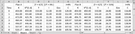
Figure 10.4 Future consumption from two investment plans with discount rate = 4 percent
From the results, Plan A is only superior to Plan B when the one-year horizon is taken using the discount rate of 4 percent.
To conclude the chapter, Dr. App says that while an individual discount rate is subjective, we can use the interest rate in the market as a proxy for a social discount rate. She also says that the decision of using short-term or long-term interest rates depends on the targeted time horizons of a project and the subjective preferences on the future consumption of each community.
Exercises
1.The file Diffusion.xls provides data on the individual indexes of the leading indicators for January through July. Construct the first diffusion index for February using a handheld calculator then continue with the indexes for the other months using Excel commands.
2.Artistown’s profit is $108,100 and grows at an annual rate of 2 percent while another school’s profit is $269,500 and grows at an annual rate of 1 percent. How long would it take for the gap between the two schools to be eliminated in the future?
3.Use the same information in Exercise (2) except the growth rate of Artistown. Find out how fast Artistown has to grow annually to eliminate the gap in two years.
4.Use the same information in Exercise (2) except the growth rate of Artistown. Find out the growth rate of Artistown that will keep the gap between the two schools the same in the next two years.
5.Consider three different investment ratios of 0, 8, and 40 percent. Assume that the capital output ratio is 2, and that there is no depreciation rate, government spending, or discount rate. The initial capital stock equals 300.
a.Construct a table similar to Figure 10.3 up to eight years using a handheld calculator or an Excel spreadsheet.
b.When does the second policy become superior to the first in welfare enhancement? When does the third policy become superior to the second?
c.What could have made the results more realistic?