
Chapter 16. Flow control patterns
In the previous chapters, you learned how to decompose systems into smaller pieces and how these pieces communicate to solve greater tasks. One aspect we have left out so far is that in addition to who interacts with whom, you must also consider the timeliness of communication. In order for your system to be resilient to varying loads, you need mechanisms that prevent components from failing uncontrollably due to overwhelming request rates. This chapter therefore introduces four basic patterns:
- The Pull pattern propagates back pressure from consumers to producers.
- The Managed Queue pattern makes back pressure measurable and actionable.
- The Drop pattern protects components under severe overload conditions.
- The Throttling pattern helps you avoid overload conditions where possible.
There are many variations on these patterns and a lot of applicable theory to be studied (in particular, control theory and queueing theory), but a treatment of these fields of research is outside the scope of this book. We hope you will be inspired by the basics presented in this chapter and refer to the scientific literature for in-depth coverage.
16.1. The Pull pattern
Have the consumer ask the producer for batches of data.
One challenge in Reactive systems is how to balance the relationship between producers and consumers of messages—be they requests that need processing or facts on their way to persistent storage. The difficulty lies in the dynamic nature of the problems that may arise from incorrect implementations: only under realistic input load can you observe whether a fast producer might overwhelm a resource-constrained consumer. Often, your load test environments are based on business forecasts that may be exceeded in real usage.
The formulation of the Pull pattern presented here is the result of Roland’s involvement in the Reactive Streams initiative,[1] where the resulting behavior is also characterized as dynamic push–pull, an aspect that we will discuss later.
See www.reactive-streams.org (version 1.0.0, published April 30, 2015).
16.1.1. The problem setting
As an illustration of a case that clearly needs flow control, suppose you want to compute the alternating harmonic series:
- 1 - 1/2 + 1/3 - 1/4 ... (converges toward the natural logarithm of 2)
Generating the input for the terms that are to be computed is as simple as emitting the series of all natural numbers, but the more costly operation is to invert each of these with high precision and then sum them with the correct signs. For the sake of simplicity, you will keep the number generation and summation within one manager actor and distribute the sign-correct inversion across a number of worker actors. These worker actors are child actors of the manager: the number generator controls the entire process and terminates when the desired precision has been reached.
The task: Your mission is to implement both the manager and the worker actors such that each worker signals demand for work in batches of 10 whenever the number of outstanding work items is less than 5.
16.1.2. Applying the pattern
We will first consider the worker actor, because in this pattern it is the active party. The worker starts the process by asking for the first batch of inputs, and when it has processed enough of them, it keeps the process going by asking for more. Multiple workers can ask the manager for inputs independently, a fact that you will use to scale out the processing across multiple CPU cores. A worker has to manage two concerns: keeping track of how much work it has already asked for and how much it has received so far, and performing the actual computation, as illustrated in the following listing.
Listing 16.1. Processing expensive calculations in a worker that pulls inputs

The numbers used here are obviously tunable to the problem and resources at hand. It is important to note that you do not implement a stop–wait scheme in which the worker pulls, then waits for the data, then computes, then replies, and then pulls again. Instead, the worker is more proactive in requesting an entire batch of inputs in one go and then renews the request when the number of outstanding work items becomes low again. In this way, the worker’s mailbox never grows beyond 14 items (requesting 10 when 4 are outstanding, and then miraculously not receiving any CPU time until those arrive—this is the worst-case scenario). It also ensures that if the worker outperforms the manager, there will always be outstanding demand signaled such that the manager can send new work immediately.
The manager shown in listing 16.2 needs to implement the other side of the Pull pattern, sending a number of work items according to each request it gets from one of the workers. The important part is that both need to agree on the notion of how much work is outstanding—requests for work must eventually be satisfied, lest the system get stuck with the worker waiting for work and the manager waiting for demand. In this example, the implementation can trivially ensure this property by always satisfying every work request immediately and in full.
Listing 16.2. Supplying a worker with tasks as it asks for them
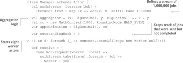

The manager only starts the workers. From then on, it is passively driven by their requests for work and their computation results. Once the stream of work items has been processed completely, the manager terminates the application after printing the final approximation result to the console.
16.1.3. The pattern, revisited
We have illustrated the case of an arbitrarily fast producer and slow consumers by distributing a computation over a group of worker actors. Were you to implement the manager such that it distributed all work items at once, you would find a few problems:
- Given enough work items (or larger ones than in this simple example), the system would run out of memory early in the process, because the work items would accumulate in the workers’ mailboxes.
- An even distribution decided up front would result in uneven execution, with some actors finishing their share later than others. CPU utilization would be lower than desired during that time period.
- If a worker failed, all of its allocated work items would be lost—the manager would need to send them again to some other worker. With the current scheme, the amount of memory to store the currently outstanding computation jobs is strictly limited, whereas with up-front distribution, it might exceed available resource limits.
You avoid these issues by giving the workers control over how much work they are willing to buffer in their mailbox, while at the same time giving the manager control over how much work it is willing to hand out for concurrent execution.
One very important aspect in this scheme is that work is requested in batches and proactively. Not only does this save on messaging cost by bundling multiple requests into a single message, but it also allows the system to adapt to the relative speed of producer and consumer:
- When the producer is faster than the consumer, the producer will eventually run out of demand. The system runs in “pull” mode, with the consumer pulling work items from the producer with each request it makes.
- When the producer is slower than the consumer, the consumer will always have demand outstanding. The system runs in “push” mode, where the producer never needs to wait for a work request from the consumer.
- Under changing load characteristics (by way of deployment changes or variable usage patterns), the mechanism automatically switches between the previous two modes without any further need for coordination—it behaves as a dynamic push–pull system.
The other notable aspect of this pattern is that it enables the composition of flow--control relationships across a chain of related components. Via the presence or absence of demand for work, the consumer tells the producer about its momentary processing capacity. In situations where the producer is merely an intermediary, it can employ the Pull pattern to retrieve the work items from their source. This implements a nonblocking, asynchronous channel over which back pressure can be transmitted along a data-processing chain. For this reason, this scheme has been adopted by the Reactive Streams standard.
16.1.4. Applicability
This pattern is well suited for scenarios where an elastic worker pool processes incoming requests that are self-contained and do not depend on local state that is maintained on each worker node. If requests need to be processed by a specific node in order to be treated correctly, the Pull pattern may still be used, but then it needs to be established between the manager and each worker individually: sending a request to the wrong worker just because it has processing capacity available would not lead to the correct result.
16.2. The Managed Queue pattern
Manage an explicit input queue, and react to its fill level.
One of the conclusions drawn from analyzing the Pull pattern is that it can be used to mediate back pressure across multiple processing steps in a chain of components. Transmitting back pressure means halting the entire pipeline when a consumer is momentarily overwhelmed, which may, for example, be caused by unfair scheduling or other execution artifacts, leading to avoidable inefficiencies in the system.
This kind of friction can lead to “stuttering” behavior in a processing engine, where short bursts of messages alternate with periods of inactivity during which back pressure signals travel through the system. These bursts can be smoothed out by employing buffers that allow the data to keep flowing even during short back pressure situations. These buffers are queues that temporarily hold messages while remembering their ordering. We call them managed queues because their use extends beyond this direct benefit: queues can be used to monitor and steer the performance of a messaging system. Buffering and managed queues are even more important at the boundaries of a system that employs back pressure: if data or requests are ingested from a source that cannot be slowed down, you need to mediate between the bounded internal capacity and the potentially unbounded influx.
16.2.1. The problem setting
In the example of the Pull pattern, you implemented a manager that had the formula for creating all required work items. Now, you will consider the manager to be just a mediator, with the source of the work items outside of its control: the manager will receive work requests while maintaining the Pull pattern with its workers. In order to smooth out the behavior in the case of momentary lack of requests from the workers, you will install a buffer within the manager.
The task: Your mission is to adapt the worker and manager actors from the Pull pattern example such that the numbers to be inverted are generated externally. The manager will keep a buffer of no more than 1,000 work items, responding with a rejection message to work items that are received while the buffer is full.
16.2.2. Applying the pattern
The main part you need to change is the manager actor. Instead of generating work items on demand, it now needs to hold two queues: one for work items while all workers are busy and one for workers’ requests when no work items are available. An example is shown next.
Listing 16.3. Managing a work queue to react to overload
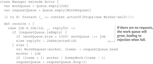
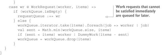
Because you would like to use workers in round-robin fashion in this example, a case arises that requires an adaptation of the protocol between manager and worker: when satisfying a queued work request from a received job, you need to follow up the Job message with a DummyWork message that tells the worker that the remaining requested work items will not be sent. This leads to the worker sending a new request very soon and simplifies the manager’s state management. You do so because the interesting point lies not with the management of the requestQueue but with the workQueue: this queue holds the current knowledge of the manager with respect to its workers’ load situation. This queue will grow while the external producer outpaces the pool of workers, and it will shrink while workers catch up with the external requests. The fill level of this queue can thus be used as a signal to steer the worker pool’s size, or it can be used to determine whether this part of the system is overloaded—you implement the latter in this example.
The worker actor does not need to change much, compared to the Pull pattern; it only needs to handle the DummyWork message type:
class Worker(manager: ActorRef) extends Actor {
  ...

  def receive = {
    ...
    case DummyWork(count) =>
      requested -= count
      request()
  }
}
16.2.3. The pattern, revisited
You have used the Pull pattern between the manager and its workers and made the back pressure visible by observing the fill level of a queue that is filled with external requests and emptied based on the workers’ demands. This measurement of the difference between requested and performed work can be used in many ways:
- We have demonstrated the simplest form, which is to use the queue as a smoothing buffer and reject additional requests while the queue is full. This implements service responsiveness while placing an upper bound on the size of the work queue.
- You could spin up a new worker once a given high–water mark was reached, adapting the worker pool elastically to the current service usage. Spinning down extraneous workers could be done by observing the size of the requestQueue as well.
- Rather than observe the momentary fill level of the queue, you could instead monitor its rate of change, taking sustained growth as a signal to enlarge the pool and sustained decrease as a signal to shrink it again.
This list is not exhaustive. There is an entire field of research called control theory[2] around the issue of how to steer process characteristics based on continuous measurements and reference values.
See, for example, https://en.wikipedia.org/wiki/Control_theory.
16.2.4. Applicability
Using managed queues instead of using implicit queues as discussed in section 2.1.3 is always desirable, but it does not need to be done at every step in a processing chain. Within domains that mediate back pressure (for example, by using the Pull pattern), buffers often have the primary function of smoothing out bursts. Observable or intelligent queues are used predominantly at the boundaries of such a system, where the system interacts with other parts that do not participate in the back pressure mechanism. Note that back pressure represents a form of coupling, and as such its scope must be justified by the requirements of the subsystem it is applied to.
Applying intelligent queues is fun and invites forays into advanced control-theory concepts, feedback loops, self-tuning systems, and so on. Although this can be a stimulating learning experience, it also makes the system more complex and presents a barrier for newcomers to understand why and how it works. Another consideration is that the theoretical equations that describe the system’s behavior become ever more complex the more numerous the active elements are within it, so going overboard with this pattern will defeat its purpose and likely lead to more erratic system behavior and suboptimal throughput and latency characteristics. Typical symptoms of having too much “intelligence” built into the system are oscillations in the decisions of the regulatory elements, which lead to potentially fatal oscillations in the system’s behavior—scaling up and down too quickly and too frequently and sometimes hitting hard resource limits or failing completely.
16.3. The Drop pattern
Dropping requests is preferable to failing uncontrollably.
Imagine a system that is exposed to uncontrollable user input (for example, a site on the internet). Any deployment will be finite in both its processing capability and its buffering capacity, and if user input exceeds the former for long enough, the latter will be used up and something will need to fail. If this is not foreseen explicitly, then an automatic out-of-memory killer will make a decision that is likely to be less satisfactory than a planned load-shedding mechanism—and shedding load means dropping requests.
This is more of a philosophy than an implementation pattern. Network protocols, operating systems, programming platforms, and libraries will all drop packets, messages, or requests when overloaded; they do so in order to protect the system so that it can recover when load decreases. In the same spirit, authors of Reactive systems need to be comfortable with the notion of sometimes deliberately losing messages.
16.3.1. The problem setting
We will revisit the example from the Managed Queue pattern, where the source of requests is situated outside of your control. When work items are sent to the manager faster than workers can process them, the queue will grow, and eventually JobRejected messages will be sent back. But even this can only happen at a certain maximum rate; when jobs are sent at a higher rate, the manager’s mailbox will begin to grow, and it will do so until the system runs out of memory.
The task: Your mission is to adapt the manager actor such that it accepts all work items into its queue up to a queue size of 1,000 and drops work items without sending back a response when the incoming rate exceeds the workers’ capacity by more than a factor of 8.
16.3.2. Applying the pattern
The modification you are seeking to make will require two levels of rejection: past a queue size of 1,000, you will send back rejections; but you still need to keep track of the incoming rate in order to stop sending rejections when the incoming rate is more than 8 times the worker pool’s capacity. But how can you do that?
If you keep the scheme from the Managed Queue pattern of not enqueueing work when the queue size has reached 1,000, then you will need to introduce another data structure that maintains the rate information: you will need to track WorkRequest messages in order to know how fast workers can process their work items, and you will need to track rejections to measure the excess rate of incoming work items. The data structure will need current timestamps for every piece of information that is fed into it, and it will need to know the current time when asking for a decision about whether to drop an item. All this is possible to implement, but doing so has a cost both at development time and at runtime—looking at the clock does not come free, plus the data structure will consume space and require CPU time to remain up to date.
Looking back at the manager actor, you see a data structure whose usage you can change slightly to provide the required information: the queue can always tell you about its length, and you can make it so the queue length reflects the excess rate. The key to this trick is that for a slowly changing incoming rate, the queue fill level will stabilize if there is a point at which ingress and egress are balanced: when workers pull items out at the same rate items enter the queue, both will even out. To make this work, you must decouple the incoming work-item rate from the enqueueing rate—you assume the worker pool’s capacity to be constant, so the enqueueing rate is all you can work with.
The solution to this riddle to keep enqueueing in general, but for every item, you roll the dice to decide whether it gets in. The probability of being enqueued must decrease with growing queue size, as shown in figure 16.1: a longer queue results in fewer items getting in. The ratio between the two is the probability for the dice roll, and at the same time it matches the ratio of excess rate to worker-pool rate.
Figure 16.1. The probability of enqueueing incoming work items into the managed queue decreases once the nominal size has been reached.
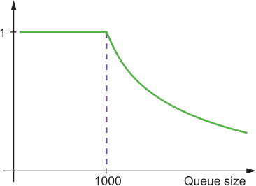
It is instructive to conduct a thought experiment to understand how and why this works. Assume that the system starts with an empty queue and a rate mismatch of a factor of 10. The queue will quickly become full (reach 1,000 elements), at which point rejections will be generated. But the queue will continue to grow—only more slowly, due to the probabilistic enqueueing. Once the queue size is so big that the enqueueing probability drops to 10%, the enqueueing rate will match the dequeueing rate, and the size of the queue will remain stable until either the external work-item rate or the worker-pool capacity changes.
In terms of code, not much is needed to implement this scheme, as you can see here:
val queueThreshold = 1000
val dropThreshold = 1384
def random = ThreadLocalRandom.current

def shallEnqueue(atSize: Int) =
  (atSize < queueThreshold) || {
    val dropFactor = (atSize - queueThreshold) >> 6
    random.nextInt(dropFactor + 2) == 0
  }
You use this logic to handle incoming Job messages:
case job @ Job(id, _, replyTo) =>
  if (requestQueue.isEmpty) {
    val atSize = workQueue.size
    if (shallEnqueue(atSize)) workQueue :+= job
    else if (atSize < dropThreshold) replyTo ! JobRejected(id)
  } else ...
This means you will enqueue a certain fraction of incoming jobs even when the queue size is greater than 1,000, and the probability of enqueueing a given job decreases with growing queue size. At size 1,000, dropFactor is 0, and the probability of picking a zero from nextInt(2) is 50%. At size 1,064, dropFactor is 1, and the probability decreases to 33%—and so on, until at the drop threshold of 1,384, the probability is 1/8. dropThreshold is therefore chosen such that the desired cutoff point for rejection messages is implemented.
16.3.3. The pattern, revisited
The example includes two modes of overload reactions: either you send back an incomplete response (degraded functionality), or you do not reply at all. You implement the metric for selecting one of these modes based on the work-item queue the manager maintains. For this, you need to allow the queue to grow past its logical capacity bound, where the excess is regulated to be proportional to the rate mismatch between producers and consumers of work items—by choosing a different formula for dropFactor, you could make this relation quadratic, exponential, or whatever is required.
The important piece here is that providing degraded functionality only works up to a given point, and the service should foresee a mechanism that kicks in once this point is reached. Providing no functionality at all—dropping requests—is cheaper than providing degraded functionality, and under severe overload conditions this is all the service can do to retain control over its resources.
One notable side effect of the chosen implementation technique is that during an intense burst, you now enqueue a certain fraction of work items, whereas the strictly bounded queue as implemented in the Managed Queue pattern example would reject the entire burst (assuming that the burst occurs faster than consumption by the workers).
Extension to implicit queues
We have so far only regarded the behavior of the explicit queue maintained by the manager actor. This actor, however, has only finite computing resources at its disposal, and even the calculations for deciding whether to drop a message have a certain cost. If the incoming rate is higher than the manager actor can decide about, its mailbox will grow: over time, it will eat up the JVM heap and lead to fatal termination through an OutOfMemoryError. This can only be avoided by limiting the implicit queues—the manager’s mailbox, in this case—in addition to the explicit queues.
Because you are dealing with an aspect that is implicitly handled by the framework (Akka, in this example), you do not need to write much code to implement this. You only need to instruct Akka to install a bounded mailbox for the manager actor:
val managerProps = Props(new Manager).withMailbox("bounded-mailbox")
When this description is used to create the manager actor, Akka will look in its configuration for a section describing the bounded mailbox. The following settings configure a mailbox that is bounded to 1,000 messages:
bounded-mailbox {
  mailbox-type = "akka.dispatch.BoundedMailbox"
  mailbox-capacity = 1000
  mailbox-push-timeout-time = 0s
}
This has an important drawback: this mailbox drops not only Job messages from external sources but also WorkRequest messages from the worker actors. In order to make those cope with such losses, you must implement a resending mechanism (which would be needed in any case, if the workers were deployed remotely), but this will not fix a more severe issue. For example, if the external rate is 10 times as high as what can be processed, then only 1 in 10 work requests will make it back, leading to workers idling because they cannot tell the manager about their demand as quickly as they need to.
This demonstrates that dropping at a lower level will always be less precise than dropping at the level that has all the necessary information, but it is the nature of overload situations that this knowledge can be too costly to maintain. The bounded mailbox in Akka is well suited for actors that do not need to communicate with other actors in the course of handling their main input, but it has weaknesses for manager-like scenarios.
To protect the manager actor with a bounded mailbox, you have to keep that mailbox separate from the one used to communicate with worker actors. Because every actor can have only one mailbox, this means installing another actor, as shown in figure 16.2.
Figure 16.2. Placing an actor with a bounded mailbox in front of the manager actor requires that the manager uses a non-message-based back channel to signal that it has received a given message. In this fashion, the incoming queue can remain strictly bounded.

The IncomingQueue actor will be configured to use the bounded mailbox, which protects it from extremely fast producers. Under high load, this actor will constantly be running, pulling work items out of its mailbox and sending them on to the manager actor. If this happens without feedback, the manager can still experience unbounded growth of its own mailbox, but you cannot use actor messages to implement the feedback mechanism. In this case, it is appropriate to consider the deployment to be local—only in this case is it practically possible to run into the envisioned overload scenario—and therefore the manager can communicate with the incoming queue also using shared memory. A simple design is shown in the following listing:
private case class WorkEnvelope(job: Job) {
  @volatile var consumed = false
}

private class IncomingQueue(manager: ActorRef) extends Actor {
  var workQueue = Queue.empty[WorkEnvelope]
  def receive = {
    case job: Job =>
      workQueue = workQueue.dropWhile(_.consumed)
      if (workQueue.size < 1000) {
        val envelope = WorkEnvelope(job)
        workQueue :+= envelope
        manager ! envelope
      }
  }
}
The only thing the manager has to do is set the consumed flag to true upon receipt of a WorkEnvelope. Further improvements that are omitted for the sake of simplicity include cleaning out the incoming queue periodically, in case there are long pauses in the incoming request stream during which work items would be unduly retained in memory. The full code for this example can be found with the book’s downloads in the file DropPatternWithProtection.scala.
Although this extension seems specific to Akka, it is generic. In any OS and service platform, there will be implicit queues that transport requests from the network to local processes as well as within these processes—these could be message queues, thread pool task queues, threads that are queued for execution, and so on. Some of these queues are configurable, but changing their configuration will have indiscriminate effects on all kinds of messages passing through them; we noted earlier that the necessary knowledge exists at a higher level, but that higher level may need protection from lower levels that can only make coarse-grained decisions. The workarounds differ; the Akka example given in this section is tailored to this particular case, but the need to apply such custom solutions will arise wherever you push a platform to its limits.
16.3.4. Applicability
During system overload, some kind of failure is bound to happen. Determining what kind it will be is a business decision: should the system protect itself by foregoing responsiveness, or should it come to a crawling but uncontrolled halt when resources are exhausted? The intuitive answer is the former, whereas typical engineering practice implements the latter—not deliberately, but due to neglect resulting from other aspects of the application design having higher priority. This pattern is always applicable, if only in the sense that not shedding load by dropping requests should be a well-understood and deliberate decision.
16.4. The Throttling pattern
Throttle your own output rate according to contracts with other services.
We have discussed how each component can mediate, measure, and react to back pressure in order to avoid uncontrollable overload situations. With these means at your disposal, it is not just fair but obligatory that you respect the ingestion limits of other components. In situations where you outpace consumers of your outputs, you can slow to match their rate, and you can even ensure that you do not violate a prearranged rate agreement.
In section 12.4.2, you saw that a circuit breaker can be designed such that it rejects requests that would otherwise lead to a request rate that is too high. With the Pull pattern, you can turn this around and not generate requests more quickly than they are allowed to be sent.
16.4.1. The problem setting
Borrowing from the Pull pattern example, suppose you have a source of work items from which you can request work. We will demonstrate the Throttling pattern by combining this source with the worker-pool implementation from the Managed Queue pattern example. The goal is to transfer work items at a rate the pool can handle so that, under normal conditions, no jobs are rejected by the managed queue.
The task: Your mission is to implement a CalculatorClient actor that pulls work from the work source and forwards it to the worker-pool manager such that the average rate of forwarded messages does not exceed a configurable limit. Bonus points are awarded for allowing short bursts of configurable size in order to increase efficiency.
16.4.2. Applying the pattern
A commonly used rate-limiting algorithm is called token bucket.[3] It is usually employed to reject or delay network traffic that exceeds a certain bandwidth allocation. The mechanism is simple:
See, for example, https://en.wikipedia.org/wiki/Token_bucket.
- A bucket of fixed size is continually filled with tokens at a given rate. Tokens in excess of the bucket size are discarded.
- When a network packet arrives, a number of tokens corresponding to the packet’s size should be removed from the bucket. If this is possible, then the packet travels on; if not, then the packet is not allowed through.
Depending on the size of the bucket, a burst of packets might be admitted after a period of inactivity; but when the bucket is empty, packets will either be dropped or delayed until enough tokens are available.
You will have to adapt this algorithm slightly in order to use it for your purposes. First, each work item carries the same weight in this example, so you require just one token per message. Second, messages do not just arrive at the actor: you must request them from the work source. Because you do not wish to drop or delay messages—where the latter would imply buffering that you want to avoid where possible—you must not request more work items from the source than you can permit through based on the current fill level of the token bucket. In the worst case, you must assume that all work items arrive before the bucket gains another token. Using the Worker actor from listing 16.1 (the Pull pattern example) as a basis, you arrive at the following implementation.
Listing 16.4. Pulling work according to a specified rate using a token bucket
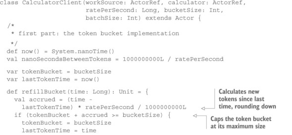
The code for the actor is organized into three parts: the first manages the token bucket, the second derives the work requests to be sent from the currently outstanding work items and the bucket fill level, and the third forwards received work items while keeping the token bucket updated and requesting more work when appropriate. There are some subtleties in writing such code, pertaining to time granularity caused by the execution of the actor at discrete times that you cannot control precisely:
- The scheduler typically does not have nanosecond-level resolution, so you must foresee that the scheduled WorkRequest is delivered later than intended.
- The actor may run more frequently than the token bucket’s refill rate, which requires you to deal with fractional tokens. You avoid this by not advancing the last update time when you encounter such cases.
- Because you do not wish to involve the imprecise scheduler more than necessary, you run the token-bucket algorithm triggered by work-item activity. Hence, you must always bring the token bucket up to date before performing other operations.
With these considerations, you arrive at an efficient and precise implementation that will ensure that the average forwarded message rate will be at most ratePerSecond (slower if the source cannot deliver quickly enough), with momentary bursts that are limited to the bucket size and with best-effort request batching for pulling items out of the source.
The full source code for this example is available with the book’s downloads. Notice that the example application does not begin the process by creating a CalculatorClient actor: instead, it first performs 100,000 calculations on the worker pool using Akka Streams. Akka Streams uses the Pull pattern internally and implements strict back pressure based on it, ensuring with the chosen combinators that no more than 1,000 calculations are outstanding at any given time. This means the worker pool will not reject a single request while exercising all code paths sufficiently to trigger the JVM just-in-time compilation; afterward, a rate of 50,000 per second will not be a problem on today’s portable hardware. Without this warm-up, you would see rejections caused by the worker pool being too slow as well as measurable interruptions caused by just-in-time compilation.
16.4.3. The pattern, revisited
You have used a rate-tracking mechanism—the token bucket—to steer the demand that you used for the Pull pattern. The resulting work-item rate then is bounded by the token bucket’s configuration, allowing you to ensure that you do not send more work to another component than was agreed on beforehand. Although a managed queue lets a service protect itself to a degree (see also the discussion of the Drop pattern and its limitations), the Throttling pattern implements service collaboration where the user also protects the service by promising to not exceed a given rate. This can be used restrictively to make rejections unlikely under nominal conditions, or it can be used more liberally to avoid having to call on the Drop pattern. But neither the Managed Queue pattern nor the Drop pattern is replaced by the Throttling pattern; it is important to consider overload protection from both the consumer and producer sides.
16.5. Summary
In this chapter, we considered that communication happens at a certain rate. You learned about different ways in which this rate can be regulated and acted on:
- The Pull pattern matches the rates of producer and consumer such that the slower party sets the pace. It works without explicitly measuring time or rates.
- The Managed Queue pattern decouples the incoming and outgoing rates with a configurable leeway—the queue size—and makes the rate difference between producer and consumer measurable and actionable.
- The Drop pattern provides an escalation for the Managed Queue pattern when the rate mismatch is too big to be handled by degrading the service functionality.
- The Throttling pattern regulates a message stream’s speed according to configured rate and burstiness parameters; it is the only presented pattern that explicitly deals with time.