
Factor Analysis Platform Overview
Factor analysis models a set of observable variables in terms of a smaller number of unobservable factors. These factors account for the correlation or covariance between the observed variables. Once the factors are extracted, you perform factor rotation in order to obtain a meaningful interpretation of the factors.
Consider a situation where you have ten observed variables, X1, X2, …, X10. Suppose that you want to model these ten variables in terms of two latent factors, F1 and F2. For convenience, it is assumed that the factors are uncorrelated and that each has mean zero and variance one. The model that you want to derive is of the form:
It follows that 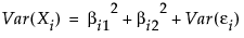 . The portion of the variance of Xi that is attributable to the factors, the common variance or communality, is
  . The remaining variance,
  , is the specific variance, and is considered to be unique to Xi.
The Factor Analysis platform provides a Scree Plot for the eigenvalues of the correlation or covariance matrix. You can use this as a guide in determining the number of factors to extract. Alternatively, you can accept the platform's suggestion of setting the number of factors equal to the number of eigenvalues that exceed one.
The platform provides two factoring methods for estimating the parameters of this model: Principal Components and Maximum Likelihood.
JMP provides two options for estimating the proportion of variance contributed by common factors for each variable. These Prior Communality options impose assumptions on the diagonal of the correlation (or covariance) matrix. The Principal Components option treats the correlation matrix, which has ones on its diagonal (or the covariance matrix with variances on its diagonal), as the structure to be analyzed. The Common Factor Analysis option sets the diagonal entries to values that reflect the proportion of the variation that is shared with other variables.
To support interpretability of the extracted factors, you rotate the factor structure. The Factor Analysis platform provides a variety of rotation methods that encompass both orthogonal and oblique rotations.
In contrast with factor analysis which looks at common variance, principal component analysis accounts for the total variance of the observed variables. See the Principal Components chapter in the Multivariate Methods book.
Example of the Factor Analysis Platform
To view an example Factor Analysis report for a data table for two factors:
1. Select Help > Sample Data Library and open Solubility.jmp.
2. Select Analyze > Consumer Research > Factor Analysis.
The Factor Analysis launch window appears.
3. Select all of the continuous columns and click Y, Columns.
4. Keep the default Estimation Method and Variance Scaling.
5. Click OK.
The initial Factor Analysis report appears.
Figure 4.2 Initial Factor Analysis Report
6. For the Model Launch, select the following options:
‒ Factoring Method as Maximum Likelihood
‒ Prior Communality as Common Factor Analysis
‒ Number of factors = 2
‒ Rotation Method as Varimax
7. After all selections are made, click Go.
The Factor Analysis report appears.
Figure 4.3 Example Factor Analysis Report
The report lists the communality estimates, variance, significance tests, rotated factor loadings, and a factor loading plot. Note that in the Factor Loading Plot, Factor 1 relates to the Carbon Tetrachloride-Chloroform-Benzene-Hexane cluster of variables, and Factor 2 relates to the Ether–1-Octanol cluster of variables. See “Factor Analysis Model Fit Options” for details of the information shown in the report.
Launch the Factor Analysis Platform
Launch the Factor Analysis platform by selecting Analyze > Consumer Research > Factor Analysis. This example uses the Solubility.jmp sample data table.
Figure 4.4 Factor Analysis Launch Window
Y, Columns
Lists the continuous columns to be analyzed.
Weight
Enables you to weight the analysis to account for pre-summarized data.
Freq
Identifies a column whose numeric values assign a frequency to each row in the analysis.
By
Creates a Factor Analysis report for each value specified by the By column so that you can perform separate analyses for each group.
Estimation Method
Lists different methods for fitting the model. For details about the methods, see the Multivariate chapter in the Multivariate Methods book.
Variance Scaling
Lists the scaling methods for performing the factor analysis based on Correlations (the same as Principal Components), Covariances, or Unscaled.
The Factor Analysis Report
The initial Factor Analysis report shows Eigenvalues and the Scree Plot. The Eigenvalues are obtained from a principal components analysis. The Scree Plot graphs these eigenvalues. The number of factors that JMP suggests in the Model Launch equals the number of eigenvalues that exceed 1.0.
Alternatively, you can use the scree plot to guide your initial choice for number of factors. The number of eigenvalues that appear before the scree plot levels out can provide an upper bound on the number of factors.
Figure 4.5 Factor Analysis Report
In the example shown in Figure 4.5, the Scree Plot begins to level out after the second eigenvalue. The Eigenvalues table indicates that the first eigenvalue accounts for 79.75% of the variation and the second eigenvalue accounts for 15.75%, for a total of 95.50% of the total variation. The third eigenvalue only explains 2.33% of the variation, and the contributions from the remaining eigenvalues are negligible. Although the Number of factors box is initially set to 1, this analysis suggests that extracting 2 factors is appropriate.
Model Launch
To configure the Factor Analysis model, use the Model Launch section at the bottom of the Factor Analysis Report (Figure 4.6).
Figure 4.6 Model Launch
The Model Launch section enables you to configure the following options:
1. Factoring method - the method for extracting factors.
‒ The Principal Components method is a computationally efficient method, but it does not allow for hypothesis testing.
‒ The Maximum Likelihood method has desirable properties and allows you to test hypotheses about the number of common factors.
Note: The Maximum Likelihood method requires a positive definite correlation matrix. If your correlation matrix is not positive definite, select the Principal Components method.
2. Prior Communality - the method for estimating the proportion of variance contributed by common factors for each variable.
‒ Principal Components (diagonals = 1) sets all communalities equal to 1, indicating that 100% of each variable’s variance is shared with the other variables. Using this option with Factoring Method set to Principal Components results in principal component analysis.
‒ Common Factor Analysis (diagonals = SMC) sets the communalities equal to squared multiple correlation (SMC) coefficients. For a given variable, the SMC is the RSquare for a regression of that variable on all other variables.
3. The Number of factors (or principal components) determined by eigenvalues greater than or equal to 1.0 or from the scree plot where the graph begins to level out.
Note: Alternatively, the Kaiser criterion retains those factors with eigenvalues greater than 1.0. In our example, only factor 1 would be retained for analysis.
4. The Rotation method to align the factor directions with the original variables for ease of interpretation. The default value is Varimax. See “Rotation Methods” for a description of the available selections.
5. Click Go to generate the Factor Analysis report.
Depending on the selected Variance Scaling, the appropriate factor analysis results appear. See “Factor Analysis Model Fit Options” for details about the contents of the report. The Factor Analysis on Correlations and Factor Analysis on Unscales reports show the same information.
Rotation Methods
Rotations align the directions of the factors with the original variables so that the factors are more interpretable. You hope for clusters of variables that are highly correlated to define the rotated factors.
After the initial extraction, the factors are uncorrelated with each other. If the factors are rotated by an orthogonal transformation, the rotated factors are also uncorrelated. If the factors are rotated by an oblique transformation, the rotated factors become correlated. Oblique rotations often produce more useful patterns than do orthogonal rotations. However, a consequence of correlated factors is that there is no single unambiguous measure of the importance of a factor in explaining a variable.
For each rotation method, we used the example described in “Example of the Factor Analysis Platform” to view the Rotated Factor Loading and Factor Loading Plot.
Orthogonal Rotation Methods
Table 4.1 lists the available orthogonal (that is, uncorrelated) rotation methods.
|
Method
|
SAS PROC FACTOR Equivalent
|
|
Varimax
|
ROTATE=ORTHOMAX with GAMMA = 1
Note: This is the default selection.
|
|
Biquartimax
|
ROTATE=ORTHOMAX with GAMMA = 0.5
|
|
Equamax
|
ROTATE=ORTHOMAX with GAMMA = number of factors/2
|
|
Factorparsimax
|
ROTATE=ORTHOMAX with GAMMA = number of variables
|
|
Orthomax
|
ROTATE=ORTHOMAX
Or
ROTATE=ORTHOMAX(p), where p is the orthomax weight or the GAMMA = value.
Note: The default p value is 1 unless specified otherwise in the GAMMA = option. For additional information about orthomax weight, see the SAS documentation, “Simplicity Functions for Rotations.”
|
|
Parsimax
|
ROTATE=ORTHOMAX with GAMMA =
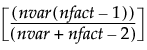 where nvar is the number of variables, and nfact is the number of factors.
|
|
Quartimax
|
ROTATE=ORTHOMAX with GAMMA=0
|
Oblique Rotation Methods
Table 4.2 lists the available oblique (that is, correlated) rotation methods.
|
Method
|
SAS PROC FACTOR
Equivalent
|
|
Biquartimin
|
ROTATE=OBLIMIN(.5)
Or
ROTATE=OBLIMIN with TAU=.5
|
|
Covarimin
|
ROTATE=OBLIMIN(1)
Or
ROTATE=OBLIMIN with TAU=1
|
|
Obbiquartimax
|
ROTATE=OBBIQUARTIMAX
|
|
Obequamax
|
ROTATE=OBEQUAMAX
|
|
Obfactorparsimax
|
ROTATE=OBFACTORPARSIMAX
|
|
Oblimin
|
ROTATE=OBLIMIN, where the default p value is zero, unless specified otherwise in the TAU= option.
ROTATE=OBLIMIN(p) specifies p as the oblimin weight or the TAU= value.
Note: For additional information about oblimin weight, see the SAS documentation, “Simplicity Functions for Rotations.”
|
|
Obparsimax
|
ROTATE=OBPARSIMAX
|
|
Obquartimax
|
ROTATE=OBQUARTIMAX
|
|
Obvarimax
|
ROTATE=OBVARIMAX
|
|
Quartimin
|
ROTATE=OBLIMIN(0) or ROTATE=OBLIMIN with TAU=0
|
|
Promax
|
ROTATE=PROMAX
|
Factor Analysis Platform Options
The Factor Analysis platform red triangle menu enables you to select to view or hide the following report elements:
Eigenvalues
A table that indicates the total number of factors extracted based on the eigenvalues (that is, the amount of variance contributed by each factor). The table includes the percent of the total variance contributed by that factor, a bar chart illustrating the percent contribution, and the cumulative percent contributed by each successive factor. The number of eigenvalues greater than or equal to 1.0 can be taken as the number of sufficient factors for analysis.
Scree Plot
A plot of the eigenvalues versus the number of components (or factors). The plot can be used to determine the number of factors that contribute to the maximum amount of variance. The point at which the plotted line levels out can be taken as the number of sufficient factors for analysis.
Script
Lists the Script menu options for the platform. See the JMP Platforms chapter in the Using JMP book for details.
See Figure 4.2 for an example.
Factor Analysis Model Fit Options
After submitting the Model Launch, the model results appear. The following options are available from the Factor Analysis report’s red triangle menu.
Prior Communality
An initial estimate of the communality for each variable. For a given variable, this estimate is the squared multiple correlation coefficient (SMC), or RSquare, for a regression of that variable on all other variables.
Note: The Prior Communality Estimates table only appears if the Common Factor Analysis (diagonals = SMC) option is selected.
Figure 4.7 Prior Communality Estimates
Eigenvalues
Shows the eigenvalues of the reduced correlation matrix and the percent of the common variance for which they account. The reduced correlation matrix is the correlation matrix with its diagonal entries replaced by the communality estimates. The eigenvalues indicate the common variance explained by the factors. The Cum Percent can exceed 100% because the reduced correlation matrix is not necessarily positive definite and can have negative eigenvalues.
Note that the table indicates the number of factors retained for analysis.
The Eigenvalues option is only available when the Prior Communality option is set to Common Factor Analysis (diagonals = SMC). The communality estimates are the SMC (square multiple correlation) values.
Figure 4.8 indicates that the first two factors account for 100.731% of the common variance. This pattern suggests that you may not need more that two factors to model your data.
Figure 4.8 Eigenvalues of the Reduced Correlation Matrix
Unrotated Factor Loading
Shows the factor loading matrix before rotation. Factor loadings measure the influence of a common factor on a variable. Because the unrotated factors are orthogonal, the factor loading matrix is the matrix of correlations between the variables and the factors. The closer the absolute value of a loading is to 1, the stronger the effect of the factor on the variable.
Use the slider and value to Suppress Absolute Loading Values Less Than the specified value in the table. Suppressed values appear dimmed according to the setting specified by Dim Text.
Use the Dim Text slider and value to control the table’s font transparency gradient for factor values less in absolute value than the specified Suppress Absolute Loading Values Less Than value.
Note: The Suppress Absolute Loading Values Less Than value and Dim Text value are the same values used in the Rotated Factor Loading table. Changes to one loading table’s settings changes the settings in the other loading table.
Figure 4.9 Unrotated Factor Loading
Note: The Unrotated Factor Loading matrix is re-ordered so that variables associated with the same factor appear next to each other.
Rotation Matrix
Shows the calculations used for rotating the factor loading plot and the factor loading matrix.
Figure 4.10 Rotation Matrix
Target Matrix
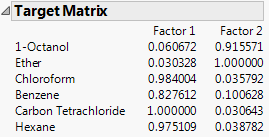
Shows the matrix to which the varimax factor pattern is rotated. This option is available only for the Promax rotation.
Figure 4.11 Target Matrix
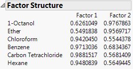
Factor Structure
Shows the matrix of correlations between variables and common factors. If the common factors are uncorrelated. This option is available only for oblique rotations.
Figure 4.12 Factor Structure
Final Communality Estimates
Estimates of the communalities after the factor model has been fit. When the factors are orthogonal, the final communality estimate for a variable equals the sum of the squared loadings for that variable.
Figure 4.13 Final Communality Estimates
Standard Score Coefficients
Lists the multipliers used to convert factor values when saving rotated components as factors to the source data table.
Figure 4.14 Standard Score Coefficients
Variance Explained by Each Factor
Gives the variance, percent, and cumulative percent, of common variance explained by each rotated factor.
Figure 4.15 Variance Explained by Each Factor
Significance Test
If you select Maximum Likelihood as the factoring method, the results of two Chi-square tests are provided.
The first test is for H0: No common factors. This null hypothesis indicates that none of the common factors are sufficient to explain the intercorrelations among the variables. This test is Bartlett’s Test for Sphericity, whose null hypothesis is that the correlation matrix of the factors is an identity matrix (Bartlett, 1954).
The second test is for H0: N factors are sufficient, where N is the specified number of factors. Rejection of this null hypothesis indicates that more factors may be required to explain the intercorrelations among the variables (Bartlett, 1954).
The tests in Figure 4.16 indicate that the common factors already included in the model explain some of the intercorrelations, but that more factors are needed.
Note: The Significance Test table only appears if the Maximum Likelihood factoring method option is selected.
Figure 4.16 Significance Test
Rotated Factor Loading
Shows the factor loading matrix after rotation. If the rotation is orthogonal, these values are the correlations between the variables and the rotated factors.
Use the slider and value to Suppress Absolute Loading Values Less Than the specified value in the table. Suppressed values appear dimmed according to the setting specified by Dim Text.
Use the Dim Text slider and value to control the table’s font transparency gradient for factor values less in absolute value than the specified Suppress Absolute Loading Values Less Than value.
Note: The Suppress Absolute Loading Values Less Than value and Dim Text value are the same values used in the Unrotated Factor Loading table. Changes to one loading table’s settings changes the settings in the other loading table.
Figure 4.17 Rotated Factor Loading
Note: The Rotated Factor Loading matrix is re-ordered so that variables associated with the same factor appear next to each other.
Factor Loading Plot
The plot of the rotated loading factors.
Figure 4.18 Factor Loading Plot
Note that in the Factor Loading Plot, Factor 1 relates to the Carbon Tetrachloride-Chloroform-Benzene-Hexane cluster of variables, and Factor 2 relates to the Ether–1-Octanol cluster of variables. See the matrix of “Rotated Factor Loading” for details.
Score Plot
The Score Plot graphs each factor’s calculated values in relation to the other adjusting each value for the mean and standard deviation.
Figure 4.19 Score Plot
Score Plot with Imputation
Imputes any missing values and creates a score plot. This option is available only if there are missing values.
Save Rotated Components
Saves the rotated components to the data table, with a formula for computing the components. The formula cannot evaluate rows with missing values.
Save Rotated Components with Imputation
Imputes missing values, and saves the rotated components to the data table. The column contains a formula for doing the imputation, and computing the rotated components. This option appears after the Factor Analysis option is used, and if there are missing values.
Remove Fit
Removes the fit model results from the Factor Analysis Fit Model report. This option enables you to change the Model Launch configuration for a new report.
..................Content has been hidden....................
You can't read the all page of ebook, please click here login for view all page.